Kinematic Cusps with Two Missing Particles II:
Cascade Decay Topology

Abstract

Three-step cascade decays into two invisible particles and two visible particles via two intermediate on-shell particles develop cusped peak structures in several kinematic distributions. We study the basic properties of the cusps and endpoints in various distributions and demonstrate that the masses of the missing particles and the intermediate particles can be determined by the cusp and endpoint positions. Effects from realistic considerations such as finite decay widths, longitudinal boost of the parent particle, and spin correlations are shown to be under control for the processes illustrated.

I Introduction

At the energy frontier, the LHC experiments are taking us to an unprecedented territory of the Tera-scale physics beyond the Standard Model (SM). At the cosmo frontier, we have entered an era of precision cosmology. With much progress made in the two frontiers, we have to admit that our understanding of the Universe is still far from being complete. According to the precise measurements of the cosmic microwave background fluctuations, such as WMAP wmap , about 95% component of the current universe has never been directly detected in the laboratory. The dominant component ($\approx 72\%$) is dark energy that is responsible for the accelerating expansion of the universe dark:energy . The second dominant ($\approx 23\%$) is cold dark matter (CDM), which is assumed to be in a form of nonrelativistic matter but cannot be explained within the SM. Albeit its extraordinary success in explaining current experimental data with incredibly high precision, the SM is regarded as an effective theory below a certain scale. For example, theoretical unnaturalness of the SM, dubbed as gauge hierarchy problem, suggests new physics beyond the SM at the TeV scale. Therefore, it is a very intriguing possibility that such CDM components may appear in new physics models.

Indeed, some new particle physics models have answers for the astrophysical question about CDM. One of the most popular scenarios is a thermal production of weakly interacting massive particles (WIMP) WIMP . In this scenario, a stable particle $X$ had been once in thermal equilibrium in the early history of the universe, but got frozen out as its reaction rate became slower than the expansion of the universe. The stability of the CDM particle over cosmic time is often due to an unbroken parity symmetry or a discrete symmetry. Under such a symmetry, the SM particle fields are in the trivial representation while new particle fields are in some nontrivial representation. The decay of the lightest new particle into SM particles is prohibited. The current observation highly suggests that the CDM particle has its mass at the electroweak scale and its couplings with a size of weak interaction. Some popular models with WIMPs are supersymmetric models with $R$ parity SUSY:DM , the universal extra dimension (UED) model with Kaluza-Klein (KK) parity DMExtraD , and the littlest Higgs model with $T$ parity DMLittleHiggs .

This WIMP with an electroweak scale mass is likely to be produced at the LHC. In hadron colliders, such weakly interacting neutral particles can be identified only by missing transverse energy. The measurement of its mass is of crucial importance to reveal the identity of the CDM, but this is a very challenging task at the LHC because such invisible particles are pair-produced with combinatoric complications and with large errors especially in jet energy measurements. In the literature, many new ideas to measure the CDM mass have been proposed Burns:Review , such as endpoint methods endpoint , polynomial methods polynomial:combine ; polynomial , and $M_{T2}$ methods MT2:original ; MT2 ; MT2:kink ; subsystem:MT2 .

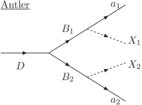
Figure 1: The antler decay topology of a parity-even particle $D$ into two missing particles ($X_{1}$ and $X_{2}$) and two visible particles ($a_{1}$ and $a_{2}$).

Recently, we have proposed a new approach to measure the missing particle mass by using the singular structures in the kinematic distributions of the antler decay cusp ; long:antler . The antler decay is a resonant decay of a parity-even particle $D$ into a pair of the missing particles ($X_{1}$ and $X_{2}$) and a pair of SM visible particles ($a_{1}$ and $a_{2}$) through two on-shell parity-odd intermediate particles ($B_{1}$ and $B_{2}$), as depicted in Fig. 1. We have studied two kinds of singular structures, an endpoint and a cusp. The positions of cusps and endpoints determine the masses of the missing particle as well as the intermediate particle, if the parent particle mass $m_{D}$ is known from other decay channels directly into two SM particles.

There are a few interesting merits of this method: (i) the positions of the cusp and endpoint are stable under the spin correlation effects since it is purely determined by the phase space; (ii) a cusp as a sharp and non-smooth peak is statistically more advantageous to search than endpoints, and more identifiable to observe than kinks; (iii) the simple configuration of outgoing particles can reduce combinatoric complication which is commonly troublesome in many missing particle mass measurement methods; (iv) the derived analytic functions for some kinematic distributions are very useful to reconstruct the mass parameters by best-fitting.

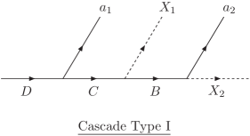
x

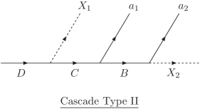
Figure 2: The cascade decay topology of a parity-even particle $D$ into two missing particles ($X_{1}$ and $X_{2}$) and two visible particles ($a_{1}$ and $a_{2}$).

In this paper, as a companion of Ref. long:antler , we focus on another decay topology with two visible particles and two missing particles from a parity-even particle $D$: cascade decays shown in Fig. 2. In this process, the parent particle $D$ sequentially decays into two particles through three steps in series, finally ended up with a missing particle $X_{2}$. There are two non-trivial types of three-step cascade decay, according to at which step the first missing particle $X_{1}$ is produced. Type I and Type II cascade decays have different cusp and endpoint structures. Unlike the symmetric antler decay case with one kind of intermediate particle, the cascade decay involves two different intermediate particles. We thus need to fix one more unknown mass, which requires more independent observables. The study of the basic properties of cusp and endpoint in various kinematic distributions to determine the unknown masses for the three-step cascade decay is our main purpose. The cusp in the invariant mass distribution of Type I decay has been discussed in the context of new physics models with the CDM particle stabilized by $Z_{3}$ symmetry Z3 .

The rest of the paper is organized as follows. In Sec. II, we categorize all possible kinematic variables from the four-momenta of the two visible particles. Section III deals with the Type I cascade decay. We present the expressions of cusps and endpoints of various kinematic distributions in a common case where $m_{a_{1}}=m_{a_{2}}=0$ and $m_{X_{1}}=m_{X_{2}}$. The functional form of the invariant mass distribution is also given. The general mass case is to be discussed in the Appendix. In Sec. IV, we present the corresponding results for the Type II cascade decay. Section V is devoted to realistic considerations such as the finite widths of the intermediate particles, the longitudinal boost of the parent particle $D$, and the spin correlation. We then conclude in Sec. VI.

II Kinematics of cascade decay topology with two missing particles

We consider the four-body cascade decay of a heavy particle $D$ through three consecutive steps. The cascade decay resulting in a single missing particle and three visible particles has been extensively studied in the literature. In the MSSM, a good example is the process of $\tilde{q}\to q\tilde{\chi}^{0}_{2}\to q\ell_{n}\tilde{\ell}\to q\ell_{n}\ell_{f}{\tilde{\chi}^{0}_{1}}$. In the UED model, we have $Q^{(1)}\to Z^{(1)}q\to L^{(1)}\ell_{n}q\to B^{(1)}\ell_{f}\ell_{n}q$. Here $\ell_{n}(\ell_{f})$ denotes the near (far) lepton with respect to the parent particle. In principle, three observable particles provide enough information to determine all the unknown mass parameters involved Burns:Review ; endpoint . However, there are some difficulties in extracting proper information, especially because of combinatoric complications. It is hard to distinguish $\ell_{n}$ from $\ell_{f}$. Furthermore, the parent particle $D$ is to be pair-produced due to its odd parity (or nontrivial representation), and thus there is always another decay chain in the same event.

Here we consider the three-step cascade decay with two missing particles. The parent particle $D$ is of even parity and thus its single production is allowed. The final states are simply two visible particles ($a_{1}$ and $a_{2}$) with missing transverse energy. There is no combinatoric complication when forming the invariant mass of two visible particles. In addition, if the rest frame of $D$ in the transverse direction can be determined, the individual transverse momenta of $a_{1}$ and $a_{2}$ in the frame also show kinematic singularities which have additional information on the mass parameters of the system. Note that this decent feature relies on the information of $D$’s transverse motion.

The cascade decays of $D\to a_{1}a_{2}X_{1}X_{2}$ can be classified according to at which step the first missing particle, say $X_{1}$, is produced. Note that we fix the other missing particle ($X_{2}$) to be produced at the last step. If $X_{1}$ is also from the last step, the final intermediate particle $B$ is just missing and this decay is indistinguishable from a two step decay. We do not consider this case. Then, there are two non-trivial three-step cascade decays, as depicted in Fig. 2. In the Type I decay, $X_{1}$ is from the second step. The parent particle $D$ decays into a visible particle $a_{1}$ and a new particle $C$, followed by the decay of $C$ into a missing particle $X_{1}$ and a new particle $B$. Finally $B$ decays into a visible particle $a_{2}$ and a missing particle $X_{2}$. In the Type II decay, $X_{1}$ is from the first step: $D$ decays into $CX_{1}$, followed by $C\to a_{1}B$, and finally $B\to a_{2}X_{2}$. In the view point of two observable particles $a_{1}$ and $a_{2}$, this Type II decay is a two-step cascade decay of a new heavy particle $C$. As shall be shown, there is no cusp structure in Lorentz-invariant distributions.

It is useful to describe the kinematics of the three-step cascade decay in terms of the rapidity of individual massive particles or a combination of multiple particles:

$$\eta^{(k)}_{i}={E^{(k)}_{i}\over m^{(k)}_{i}},$$ (1)

where $E_{i}$ and $m_{i}$ are the energy and mass of the particle (system) $i$ in the rest frame of a particle (system) $k$. To avoid confusion, we adopt the following rapidity notations for the Type I and Type II decays:

$${}\begin{array}[]{c|c|c}&\hbox{ {Type~{}I}~{}Cascade}&\hbox{ {Type~{}II}~{}Cascade}\\ \hline\cr\hbox{ rapidity notation }&\xi_{i}&\zeta_{i}\end{array}$$ (4)

For the sake of simplicity, when the rapidity is defined in the rest frame of its mother particle, we omit the superscript specifying the reference frame.

With the four-momenta $k_{1}$ and $k_{2}$ of the two observable particles $a_{1}$ and $a_{2}$ in the lab frame, respectively, we consider the following observables in three categories:

• Lorentz invariant observables: the invariant mass of $a_{1}$ and $a_{2}$,

  $$m=\sqrt{(k_{1}+k_{2})^{2}}\ .$$ (5)

• Longitudinal-boost invariant observables:

  • the magnitude of the transverse momentum of a visible particle $i$,

    $$p_{Ti}=\left|\mathbf{k}_{i}^{T}\right|,$$ (6)

  • the magnitude of the transverse momentum of the $a_{1}$-$a_{2}$ system,

    $$p_{T}=\left|\mathbf{k}_{1}^{T}+\mathbf{k}_{2}^{T}\right|,$$ (7)

  • the transverse mass of the $a_{1}$-$a_{2}$ system,

    $$m_{T}=\sqrt{p_{T}^{2}+m^{2}}\ .$$ (8)

• Non-invariant observables:

  • cosine of $\Theta_{i}$, the angle of the visible particle $a_{i}$ in the c.m. frame of $a_{1}$ and $a_{2}$, with respect to their c.m. moving direction,

    $$\cos\Theta=\frac{\mathbf{k}_{1}^{(aa)}\cdot\mathbf{k}^{(D)}}{|\mathbf{k}_{1}^{(aa)}||\mathbf{k}^{(D)}|}\ .$$ (9)

Here the bold-faced letter denotes the three-vector momentum, $k=k_{1}+k_{2}$, and the superscript $(D)$ and $(aa)$ denote the $D$-rest frame and the c.m. frame of $a_{1}$ and $a_{2}$, respectively.

As shall be shown, $p_{Ti}$ and $m_{T}$ distributions show cusp structures if the mother particle $D$ is produced at rest in the transverse direction. At a hadron collider, this is possible if $D$ is singly produced. These additional cusp structure are very valuable to determine all the unknown masses. However strong QCD interactions always yield, for example, sizable initial state radiation, which causes transverse kick to the mother particle $D$: the cusps in $p_{Ti}$ and $m_{T}$ distributions can be smeared. Caution is required when drawing the consequences for the mass measurement from these cusps. In addition, the $\cos\Theta$ distribution is defined in the rest-frame of the mother particle $D$. At a hadron collider, this is not observable. In what follows, we assume that the mother particle is produced at rest in the transverse direction.

In general, the involved seven particles ($D$, $C$, $B$, $a_{1}$, $a_{2}$, $X_{1}$, $X_{2}$) may have different masses. In many new physics models, the cascade decay processes of interest have massless visible particles and the same kind of invisible particles. For most of the presentation in the main text, therefore, we consider only the following case:

$$m_{a_{1}}=m_{a_{2}}=0,\quad m_{X_{1}}=m_{X_{2}}.$$ (10)

The result for the most general case with seven different masses is presented in the Appendix.

III Type I cascade decay

As illustrated in Fig. 2, the Type I cascade decay is the decay of a parity-even particle $D$ into two missing particles $X_{1}$ and $X_{2}$ and two visible particles $a_{1}$ and $a_{2}$ through

$$D(P)\longrightarrow C+a_{1}(k_{1}),$$

$$C\longrightarrow B+X_{1},$$

$$\hskip 34.0ptB\longrightarrow a_{2}(k_{2})+X_{2}.$$

Here the particles $D$, $C$, $a_{1}$ and $a_{2}$ are parity-even while the particles $B$, $X_{1}$, and $X_{2}$ are parity-odd. In order to accommodate the Type I cascade decay, we need at least two heavy parity-even particles.

One good example for this decay channel is in the universal extra dimension (UED) model ued . It is based on a single flat extra dimension of size $R$, compactified on an $S_{1}/Z_{2}$ orbifold. All the SM fields propagate freely in the whole five-dimensional spacetime, and each field has an infinite number of KK excited states. Since the KK parity is conserved, the lightest KK particle (LKP) with odd KK parity is stable and becomes a good candidate for the CDM. Usually the first KK mode of the $U(1)_{Y}$ gauge boson ${B^{(1)}}$ is the LKP ued ; radiative:ued . All the second KK states of the SM particles have even KK-parity and mass of $\sim 2/R$. Lower limit of $1/R\mathrel{\mathop{\kern 0.0pt\hbox to0.0pt{\raise 0.86108pt\hbox{$>$}\hss}}\lower 3.87495pt\hbox{\kern-1.90002pt$\sim$}}300$ GeV is set based on the combination of the constraints from the $\rho$ parameter rho , the electroweak precision tests EWPT , the muon $g-2$ measurement gmuon , the flavor changing neutral currents fcnc , and direct search by D0 group at the Tevatron d0 . The second KK modes are within the reach of the LHC. Possible Type I cascade decays are

$${Z^{(2)}} \to \ell_{n}+{L^{(2)}}\to\ell_{n}+{B^{(1)}}{L^{(1)}}\to\ell_{n}+{B^{(1)}}+\ell_{f}{B^{(1)}},$$ (12)

$$g^{(2)} \to q_{n}+q^{(2)}\to q_{n}+{B^{(1)}}q^{(1)}\to q_{n}+{B^{(1)}}+q_{f}{B^{(1)}}.$$ (13)

Now we present the cusps and endpoints of $m$, $m_{T}$, $p_{T}$, $p_{Ti}$, and $\cos{\Theta}$ distributions in terms of the masses. As in Eq. (10), two missing particles are of the same kind and the visible particles are massless in this case. The rapidities of the particles $B$ and $C$ in the rest frame of their mother particles are given by

$$\cosh\xi_{B}=\frac{m_{C}}{2m_{B}}\left(1+\frac{m_{B}^{2}}{m_{C}^{2}}-\frac{m_{X}^{2}}{m_{C}^{2}}\right),\quad\cosh\xi_{C}=\frac{m_{D}}{2m_{C}}\left(1+\frac{m_{C}^{2}}{m_{D}^{2}}\right).$$ (14)

We will also use $E_{n}$ and $E_{f}$, the energy of the near $a_{1}$ and the far $a_{2}$ in its mother’s rest frame, respectively:

$$E_{n}=\frac{m_{D}}{2}\left(1-\frac{m_{C}^{2}}{m_{D}^{2}}\right),\quad E_{f}=\frac{m_{B}}{2}\left(1-\frac{m_{X}^{2}}{m_{B}^{2}}\right).$$ (15)

	$m_{D}$	$m_{C}$	$m_{B}$	$m_{X}$	$\xi_{B}$
Mass–a1	1045.7	1023.	514.2	500.9	0.12
Mass–b1	600	400	200	100	0.60
Mass–c1	600	500	150	100	1.16

Table 1: Test mass spectrum sets for the Type I cascade decay. All masses are in units of GeV.

For illustration, we take three sets for the mass parameters in Table 1. The Mass–a₁ is motivated by the $Z^{(2)}$ decay in Eq. (12). The KK masses are determined by the UED model parameters of $\Lambda R=20$ and $1/R=500{\,{\rm GeV}}$, where $\Lambda$ is the cutoff scale ued . The equal spacing of the KK mode spectrum in flat extra dimension leads to very degenerate masses, i.e., $m_{D}\approx m_{C}\approx 2m_{B}\approx 2m_{X}$. The Mass–b₁ has substantial gaps for each pair of adjacent masses. Finally Mass–c₁ has a sizable mass gap between $m_{C}$ and $m_{B}+m_{X}$.

For precise mass measurements using the singularities, it is required to have a visible cusp and/or endpoint in a kinematic distribution. The visibility of the endpoints can be determined by the functional behavior near the endpoint. In what follows, the shape of an endpoint is to be classified into a fast dropping one and a long-tailed one.

(i) Invariant mass $m$ distribution: We first discuss the distribution of the invariant mass $m$ of two visible particles. The differential decay rate $d{\Gamma}/dm$ is

$$\frac{d\Gamma}{dm}\propto\begin{cases}\begin{array}[]{ll}2\xi_{B}m,&\hbox{ for }0<m<m^{\rm cusp}_{\rm cas1},\\ m\,\ln\dfrac{(m^{\rm max}_{\rm cas1})^{2}}{m^{2}},&\hbox{ for }m^{\rm cusp}_{\rm cas1}<m<m^{\rm max}_{\rm cas1},\end{array}\end{cases}$$ (16)

where the cusp and endpoint are

$$\left(m^{\rm cusp}_{\rm cas1}\right)^{2}=4E_{n}E_{f}e^{\xi_{C}-\xi_{B}},\quad\left(m^{\rm max}_{\rm cas1}\right)^{2}=4E_{n}E_{f}e^{\xi_{C}+\xi_{B}}.$$ (17)

Note that the functional behavior of $d{\Gamma}/dm$ is the same as that of the antler decay long:antler . More general case with 7 different masses is discussed in the Appendix.

Whether this cusp is sharp enough to probe can be easily deduced from Eq. (16). The $d{\Gamma}/dm$ function is linear in $m$ for $m<m^{\rm cusp}_{\rm cas1}$, and a concave function for $m^{\rm cusp}_{\rm cas1}<m<m^{\rm max}_{\rm cas1}$. At $m=m^{\rm max}_{\rm cas1}/e$, the concave function reaches its maximum. If $m^{\rm max}_{\rm cas1}/e<m^{\rm cusp}_{\rm cas1}$, which is equivalent to $\xi_{B}<1$, the cusp can be considered to be pronounced.

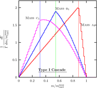
Figure 3: The normalized differential decay rate of the invariant mass of two visible particles, $\frac{d{\Gamma}}{{\Gamma}dm}$ for the Type I cascade decay. The masses are in Table 1.

In Fig. 3, we show the normalized differential decay rate of $d{\Gamma}/dm$. In order to compare the cusp shapes only, we present it as a function of $m/m^{\rm max}_{\rm cas1}$. The vertical lines denote the positions of $m^{\rm cusp}_{\rm cas1}$ in units of $m^{\rm max}_{\rm cas1}$. The Mass–a₁ case with $\xi_{B}=0.12$ has a very sharp $m$ cusp. The Mass–b₁ case with $\xi_{B}=0.60$ shows a triangular shape with a cusped peak. However, the Mass–c₁ case with $\xi_{B}=1.16$ has a dull cusp. In the $d\Gamma/dm$ distribution, the profile shape near the endpoint can be generally regarded as fast-dropping, as suggested by Eq. (16).

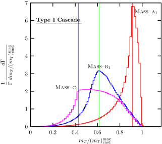
Figure 4: The normalized differential decay rate of the transverse mass of two visible particles, $\frac{d{\Gamma}}{{\Gamma}dm_{T}}$ for the Type I cascade decay. The masses are in Table 1.

(ii) Transverse mass $m_{T}$ distribution: Figure 4 shows the rate of the transverse mass $m_{T}$ distributions. For all three Mass–a₁, Mass–b₁ and Mass–c₁ cases, the $m_{T}$ distributions show visible cusp structures. It is interesting to note that the Mass–c₁ case has a more visible $m_{T}$ cusp compared with the $m$ cusp. We also note that this is contrasted to the antler decay case where there is no cusp in the $m_{T}$ distribution long:antler . As shall be shown in the next section, the Type II cascade decay also has a cusp in the $m_{T}$ distribution. Therefore, the presence of the $m_{T}$ cusp can be used for identifying the cascade decay topology. The cusp and maximum positions in terms of the masses are

$$(m_{T})^{\rm cusp}_{\rm cas1}=E_{n}+E_{f}e^{\xi_{C}-\xi_{B}},\quad(m_{T})^{\rm max}_{\rm cas1}=E_{n}+E_{f}e^{\xi_{C}+\xi_{B}},$$ (18)

where $E_{n}$ and $E_{f}$ are in Eq. (15).

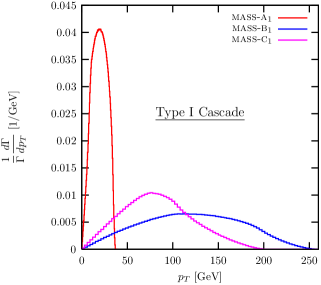
Figure 5: The normalized differential decay rate of the transverse momentum of two visible particles, $\frac{d{\Gamma}}{{\Gamma}dp_{T}}$ for the Type I cascade decay for the masses in Table 1.

(iii) The system $p_{T}$ distribution: Figure 5 shows the normalized distribution $d{\Gamma}/dp_{T}$ of the transverse momentum $p_{T}$ of two visible particles. For all three mass spectra in Table 1, the $p_{T}$ distribution has smooth peak without a cusp structure. Still the endpoint of $p_{T}$ distribution can be observed, which is

$$(p_{T})^{\rm max}_{\rm cas1} = E_{n}+E_{f}e^{-\xi_{C}+\xi_{B}}.$$ (19)

Only the Mass–a₁  case has a fast dropping endpoint shape, which is attributed to very small momentum transfer to the visible particles. More general cases of Mass–b₁ and Mass–c₁ have long-tailed endpoints. The $p_{T}$ distribution is not useful for the mass measurement.

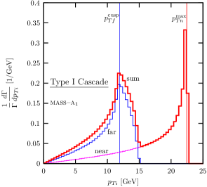
x

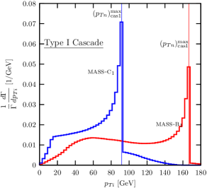
Figure 6: The normalized differential decay rate of the transverse momentum of one visible particle, $\frac{d{\Gamma}}{{\Gamma}dp_{Ti}}$ for the Type I cascade decay. In the Mass–a₁ case, the line labeled by “near” (“far”) denotes the $p_{Ti}$ distribution of $a_{1}$ ($a_{2}$). Thick lines are the summed distributions of $p_{Ti}$.

(iv) Single particle $p_{Ti}$ distribution: The individual transverse momentum $p_{Ti}$ distributions of two visible particles show unique functional behaviors, as shown in Fig. 6. The thin solid line labeled by “near” (“far”) is the $p_{Ti}$ distribution of the near visible particle $a_{1}$ (the far visible particle $a_{2}$). The $p_{Tf}$ distribution has both the cusp and the endpoint structures, while the $p_{Tn}$ distribution has only an endpoint. This $p_{Tn}$ endpoint has a sudden ending shape like a step function, which holds true for all mass cases.

In most realistic situations, one may not distinguish the near visible particle from the far one. Here we show a more practical observable, the transverse momentum of any visible particle, which becomes the sum of both $p_{Ti}$ distributions. The thick lines in Fig. 6 represent the sum

The position of the cusp and the endpoint in the $p_{Tf}$ distribution is given by

$$\left(p_{Tf}\right)^{\rm cusp}_{\rm cas1}=E_{f}e^{\xi_{C}-\xi_{B}},\quad\left(p_{Tf}\right)^{\rm max}_{\rm cas1}=E_{f}e^{\xi_{C}+\xi_{B}},$$ (20)

and the endpoint in the $p_{Tn}$ distribution is located at

$$\left(p_{Tn}\right)^{\rm max}_{\rm cas1}=E_{n},$$ (21)

where $E_{n}$, $E_{f}$, $\xi_{B}$ and $\xi_{C}$ are in Eq. (14) and (15). Depending on whether $\left(p_{Tn}\right)^{\rm max}_{\rm cas1}>\left(p_{Tf}\right)^{\rm max}_{\rm cas1}$ (the case of Mass–a₁) or not (the cases of Mass–b₁ and Mass–c₁), the summed distribution shows apparently different shape, as shown in Fig. 6. While $\left(p_{Tn}\right)^{\rm max}_{\rm cas1}$ can be easily determined due to the unique spiky feature of the distribution, the cusp and the endpoint of the $p_{Tf}$ distribution when $\left(p_{Tn}\right)^{\rm max}_{\rm cas1}<\left(p_{Tf}\right)^{\rm max}_{\rm cas1}$ is rather difficult to identify in the summed $p_{Ti}$ distribution.

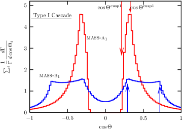
Figure 7: The summed distributions of $\cos\Theta_{i}$ in the Type I cascade decay for the masses in Table 1.

(v) $\cos\Theta$ distribution: The variable $\cos{\Theta}$ in Eq. (9) is defined by the angle of one visible particle. We have two $\cos{\Theta}$ distributions for $a_{1}$ and $a_{2}$, which cannot be distinguished. In Fig. 7, therefore, we present the summation of two $\cos{\Theta}_{i}$ distributions in the rest frame of $D$ for Mass–a₁ and Mass–b₁ cases. It is symmetric about $\cos\Theta=0$, and has two cusp structures, $\cos\Theta^{\rm cusp1}_{\rm cas1}$ and $\cos\Theta^{\rm cusp2}_{\rm cas1}$, marked by the vertical arrows. In terms of masses, they are

$$\cos\Theta^{\rm cusp1}_{\rm cas1}=\frac{E_{n}-E_{f}\exp(\xi_{B}-\xi_{C})}{E_{n}+E_{f}\exp(\xi_{B}-\xi_{C})},\quad\cos\Theta^{\rm cusp2}_{\rm cas1}=\frac{E_{n}-E_{f}\exp(-\xi_{B}-\xi_{C})}{E_{n}+E_{f}\exp(-\xi_{B}-\xi_{C})}.$$ (22)

In the Mass–a₁ case, $\cos\Theta^{\rm cusp1}_{\rm cas1}$ stands on a steep slope, which is difficult to probe. The Mass–b₁ case shows two pronounced cusps.

IV Type II cascade decay

Type II cascade decay is a chain decay of

$$D(P)\longrightarrow C+X_{1},$$

$$C\longrightarrow B+a_{1}(k_{1}),$$

$$\hskip 30.0ptB\longrightarrow a_{2}(k_{2})+X_{2}.$$

A good example can be found in the MSSM:

$$H/A\to{\tilde{\chi}^{0}_{1}}+\tilde{\chi}^{0}_{2},\quad\tilde{\chi}^{0}_{2}\to\ell_{n}+\tilde{\ell},\quad\tilde{\ell}\to\ell_{f}+{\tilde{\chi}^{0}_{1}}.$$ (24)

	$m_{D}$	$m_{C}$	$m_{B}$	$m_{X}$	$m^{\rm max}$
Mass–a2	614	299	222	161	138.0
Mass–b2	600	300	200	100	193.6
Mass–c2	400	250	150	120	120.0

Table 2: Test mass spectrum sets for the Type II cascade decay. All masses are in units of GeV.

As in the Type I cascade decay, we restrict ourselves to the realistic cascade decay with $m_{a_{1}}=m_{a_{2}}=0$ and $m_{X_{1}}=m_{X_{2}}$. Then there are two independent rapidities, $\zeta_{C}$ and $\zeta_{B}$:

$$\cosh\zeta_{B}=\frac{m_{C}}{2m_{B}}\left(1+\frac{m_{B}^{2}}{m_{C}^{2}}\right),\quad\cosh\zeta_{C}=\frac{m_{D}}{2m_{C}}\left(1+\frac{m_{C}^{2}}{m_{D}^{2}}-\frac{m_{X}^{2}}{m_{D}^{2}}\right).$$ (25)

For illustration, we take three mass sets for the Type II cascade decay in Table 2.

Figure 8: The normalized differential decay rate of the invariant mass of two visible particles, $\frac{d{\Gamma}}{{\Gamma}dm}$ for the Type II cascade decay. The mass spectrum sets are described in Table 2.

(i) Invariant mass $m$ distribution: We first study the distribution of the invariant mass of $a_{1}$ and $a_{2}$. Note that in the view point of $a_{1}$ and $a_{2}$, this Type II cascade decay is a three body decay of the parent particle $C$. The presence of the invisible $X_{1}$ decayed from $D$ does not change any Lorentz invariant result. The $m$ distribution is the same as that of, i.e., $m_{\ell\ell}$ of the decay $\tilde{\chi}^{0}_{2}\to\ell_{n}\tilde{\ell}\to\ell_{n}\ell_{f}{\tilde{\chi}^{0}_{1}}$ in the MSSM. This $m_{\ell\ell}$ distribution is well known to have no cusp structure. The endpoint is susy:mll

$$\left(m^{\rm max}_{\rm cas2}\right)^{2}=m_{C}^{2}\left(1-\frac{m_{B}^{2}}{m_{C}^{2}}\right)\left(1-\frac{m_{X}^{2}}{m_{B}^{2}}\right).$$ (26)

In Fig. 8, we show the $m$ distribution for three sets of the mass parameters in Table 2, all of which have right-angled triangle shoe without a cusp.

The absence of a cusp in a two-step cascade decay can be understood by a simple kinematic configuration. For the antler decay ($D\to B_{1}+B_{2}\to a_{1}X_{1}+a_{2}X_{2}$) in the massless visible particle case ($m_{a_{1}}=m_{a_{2}}=0$), the following four critical points correspond to a kinematic singular structure long:antler :

$${\begin{array}[]{c|c c}\hbox{1D configuration }&m_{a_{1}a_{2}}\\ \hline\cr~{}~{}~{}\stackrel{{\scriptstyle a_{2}}}{{\Longleftarrow}}~{}~{}\stackrel{{\scriptstyle B_{2}}}{{\longleftarrow}}~{}~{}\stackrel{{\scriptstyle D}}{{\bullet}}~{}~{}\stackrel{{\scriptstyle B_{1}}}{{\longrightarrow}}~{}~{}\stackrel{{\scriptstyle a_{1}}}{{\Longrightarrow}}{}{}{}&~{}~{}~{}\hbox{ max }{}{}{}\\ \stackrel{{\scriptstyle a_{2}}}{{\Longrightarrow}}~{}~{}\stackrel{{\scriptstyle B_{2}}}{{\longleftarrow}}~{}~{}\stackrel{{\scriptstyle D}}{{\bullet}}~{}~{}\stackrel{{\scriptstyle B_{1}}}{{\longrightarrow}}~{}~{}\stackrel{{\scriptstyle a_{1}}}{{\Longleftarrow}}&\hbox{ cusp }\\ \stackrel{{\scriptstyle a_{2}}}{{\Longrightarrow}}~{}~{}\stackrel{{\scriptstyle B_{2}}}{{\longleftarrow}}~{}~{}\stackrel{{\scriptstyle D}}{{\bullet}}~{}~{}\stackrel{{\scriptstyle B_{1}}}{{\longrightarrow}}~{}~{}\stackrel{{\scriptstyle a_{1}}}{{\Longrightarrow}}&\hbox{ min }\\ \stackrel{{\scriptstyle a_{2}}}{{\Longleftarrow}}~{}~{}\stackrel{{\scriptstyle B_{2}}}{{\longleftarrow}}~{}~{}\stackrel{{\scriptstyle D}}{{\bullet}}~{}~{}\stackrel{{\scriptstyle B_{1}}}{{\longrightarrow}}~{}~{}\stackrel{{\scriptstyle a_{1}}}{{\Longleftarrow}}&\hbox{ min }\\ \end{array}}$$ (32)

Here we simplify the picture as an one-dimensional case. It is clear to see that $m_{a_{1}a_{2}}^{\rm min}$ happens when two observable particles move in the same direction, while two kinematic configurations of back-to-back moving correspond to either $m_{a_{1}a_{2}}^{\rm max}$ or $m_{a_{1}a_{2}}^{\rm cusp}$. For a two-step cascade decay ($C\to a_{1}+B\to a_{1}+a_{2}X_{2}$), $a_{1}$ and $a_{2}$ in one-dimensional space have only two independent kinematic configurations, moving in the same direction and moving in the opposite direction. There is no critical point left for the cusp.

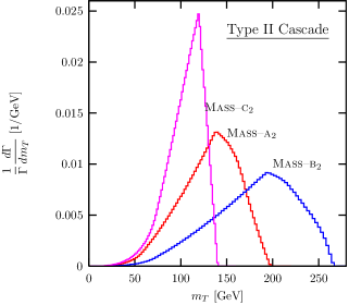
Figure 9: The normalized differential decay rate of the transverse mass of two visible particles, $\frac{d{\Gamma}}{dm_{T}}$ for the Type II cascade decay. The mass spectrum sets are described in Table 2.

(ii) Transverse mass $m_{T}$ distribution: Unlike the invariant mass distribution, the $m_{T}$ distribution contains the information about the transverse momenta of the first missing particle $X_{1}$. As shown in Fig. 9, there is a cusp here. We stress once again that this $m_{T}$ cusp appears only when $D$ is produced at rest in the transverse direction.

Another interesting feature is that the position of the $m_{T}$ cusp is nothing but the $m$ maximum:

$$(m_{T})^{\rm cusp}_{\rm cas2}=m^{\rm max}_{\rm cas2}.$$ (33)

This non-trivial equality is a unique feature of the Type II cascade decay.

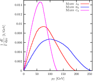
Figure 10: The normalized differential decay rate of the transverse momentum of two visible particles, $\frac{d{\Gamma}}{{\Gamma}dp_{T}}$ for the Type II cascade decay. The mass spectrum sets are in Table 2.

(iii) System $p_{T}$ distribution: The total $p_{T}$ distributions for the Type II cascade decay are shown in Fig. 10. All three mass sets have smooth $p_{T}$ distributions. And their endpoints are all long-tailed. This feature is common for the antler, Type I, and Type II cascade decay topology.

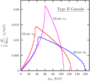
x

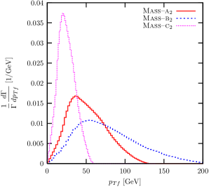
Figure 11: The normalized differential decay rate of the transverse mass of one visible particle, $\frac{d{\Gamma}}{{\Gamma}d{p_{Ti}}}$ for the Type II cascade decay. The left figure is for the near visible particle $a_{1}$, and the right one is for the far visible particle $a_{2}$.

(iv) Single particle $p_{Ti}$ distribution: Figure 11 shows the distribution of the individual transverse momentum of the near $a_{1}$ and the far $a_{2}$. The near $p_{Tn}$ distribution has a sharp cusp and a fast dropping endpoint. However the $p_{Tf}$ distribution has a long tailed endpoint without any cusp. In terms of masses they are simply

$$(p_{Tn})^{\rm cusp}_{\rm cas2}=\frac{m_{C}}{2}\left(1-\frac{m_{B}^{2}}{m_{C}^{2}}\right)e^{-\zeta_{C}},\quad(p_{Tn})^{\rm max}_{\rm cas2}=\frac{m_{C}}{2}\left(1-\frac{m_{B}^{2}}{m_{C}^{2}}\right)e^{\zeta_{C}}.$$ (34)

Note that the product of $(p_{Tn})^{\rm cusp}_{\rm cas2}$ and $(p_{Tn})^{\rm max}_{\rm cas2}$ removes the $\zeta_{C}$ dependence, which depends on the intermediate masses $m_{C}$ and $m_{B}$. In addition the ratio $(p_{Tn})^{\rm cusp}_{\rm cas2}/(p_{Tn})^{\rm max}_{\rm cas2}$ depends only on the rapidity $\zeta_{C}$.

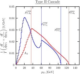
Figure 12: The sum of two normalized differential decay rate with respect to the individual transverse momenta of the near and far visible particles.

As discussed before, the individual $p_{Ti}$ distribution cannot be constructed. Instead we show the sum of two distributions in Fig. 12. For the Mass–a₂ case, the cusp in the $p_{Tn}$ distribution and the smooth peak of the $p_{Tf}$ distribution are located nearby. In their sum, the $p_{Tn}$ cusp survives over the relatively round $p_{Tf}$ peak and the fast dropping $p_{Tn}$ endpoint is also measurable. For the Mass–c₂ case, however, the $p_{Tn}$ cusp and the $p_{Tf}$ peak are separated so that the summed distribution shows both. With finite number of data, it would be difficult to distinguish the $p_{Tn}$ cusp from the $p_{Tf}$ peak.

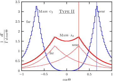
Figure 13: The sum of $d{\Gamma}/d\cos\Theta_{i}$ for the Type II cascade decay.

(v) $\cos\Theta$ distribution: We consider the $\cos\Theta$ distribution for the Type II cascade decay. In Fig. 13 we show the normalized $d{\Gamma}/d\cos\Theta$ for the near and far visible particles (denoted by thin lines) as well as their sum (thick lines) for the Mass–A₂ and Mass–C₂. In both cases, the summed distribution of $\cos{\Theta}_{i}$ is symmetric about $\cos{\Theta}=0$, and has one independent sharp cusp denoted by vertical lines in Fig. 13. The $\cos{\Theta}$ cusp position in terms of the mass parameters is

$$\cos\Theta^{\rm cusp}_{\rm cas2}=\frac{m_{C}\left(1-\frac{m_{B}^{2}}{m_{C}^{2}}\right)-m_{B}\left(1-\frac{m_{X}^{2}}{m_{B}^{2}}\right)e^{-\zeta_{B}}}{m_{C}\left(1-\frac{m_{B}^{2}}{m_{C}^{2}}\right)+m_{B}\left(1-\frac{m_{X}^{2}}{m_{B}^{2}}\right)e^{-\zeta_{B}}}.$$ (35)

(vi) Mass determination from the cusps and endpoints: Unlike the antler decay with one kind of intermediate particles, the cascade decay has two different intermediate particles. In addition, the Type II decay has fewer independent observables of cusps and endpoints. First there is no $m$ cusp structure. Second the $m_{T}$ cusp position is the same as the $m$ endpoint. A natural concern arises whether we have enough information to determine all the masses, especially at the LHC where the $\cos\Theta$ cusp cannot be used. Fortunately three unknown masses ($m_{C}$, $m_{B}$, and $m_{X}$) are unambiguously determined by three observables of $m^{\rm max}_{\rm cas2}$, $(p_{Tn})^{\rm cusp}_{\rm cas2}$, and $(p_{Tn})^{\rm max}_{\rm cas2}$:

$$m_{C} = R_{\alpha}m_{D},\quad m_{B}=\sqrt{1-\frac{\alpha_{1}}{R_{\alpha}}}\;m_{C},\quad m_{X}=\sqrt{1-\frac{\alpha_{2}}{R_{\alpha}}}\;m_{B},$$ (36)

where $R_{\alpha}$ is

$$R_{\alpha} = \frac{1+{\alpha}_{1}{\alpha}_{2}}{{\alpha}_{3}-{\alpha}_{1}-{\alpha}_{2}},$$ (37)

and ${\alpha}_{1,2,3}$ are

$$\alpha_{1} = \frac{(m^{\rm max}_{\rm cas2})^{2}}{2m_{D}\sqrt{{(p_{Tn})^{\rm max}_{\rm cas2}}/{(p_{Tn})^{\rm cusp}_{\rm cas2}}}},$$ (38)

$${}\alpha_{2} = \frac{2\sqrt{(p_{Tn})^{\rm max}_{\rm cas2}/(p_{Tn})^{\rm cusp}_{\rm cas2}}}{m_{D}},$$

$${}\alpha_{3} = \sqrt{\frac{(p_{Tn})^{\rm max}_{\rm cas2}}{(p_{Tn})^{\rm cusp}_{\rm cas2}}}+\sqrt{\frac{(p_{Tn})^{\rm cusp}_{\rm cas2}}{(p_{Tn})^{\rm max}_{\rm cas2}}}.$$

V Effects of realistic considerations

All the previous expressions of the cusps and endpoints have been derived in an idealistic situation: the total decay widths of decaying particles are ignored; the $D$ rest frame is assumed to be reconstructed; the spin-correlation effects from the full matrix elements are negligible. In this section, we investigate these effects on the position and shape of each kinematic cusp and endpoint.

V.1 Finite width effects

Up to now we have applied the narrow width approximation, ignoring the width of decaying particles. Since the effect of finite ${\Gamma}_{D}$ is very minor cusp , we focus on the effects of ${\Gamma}_{B}$ and ${\Gamma}_{C}$.

Figure 14: The finite decay width effects on the $m$ and $m_{T}$ distributions in the Mass–a₁ case. Solid lines are for the on-shell decay, the long dashed lines for ${\Gamma}/M=0.01$, the short dashed lines for ${\Gamma}/M=0.1$, and the dotted lines for ${\Gamma}/M=0.5$. Here ${\Gamma}/M\equiv{\Gamma}_{B}/M_{B}={\Gamma}_{C}/M_{C}$.

Figure 15: The finite decay width effects on the summed distributions of $p_{Ti}$ and $\cos\Theta_{i}$ in the Mass–a₁ case of the Type I cascade decay. As before, we take ${\Gamma}/M=0,~{}0.01,~{}0.1,~{}0.5$.

We find that the mass spectrum is the most crucial factor to determine the stability of the cusp and endpoint structures under the width effects. Out of six cases in Tables 1 and 2, the Mass–a₁ has very vulnerable structures. This case is special because of its degenerate masses: the observable particles have very small momentum transfer and their kinematic phase space is highly limited.

In Fig. 14 and Fig. 15, we show the finite width effects for the Mass–a₁ case. We present four cases for ${\Gamma}_{B}$ and ${\Gamma}_{C}$: on-shell (solid line), ${\Gamma}/M=0.01$ (long dashed line), ${\Gamma}/M=0.1$ (short dashed lien), and ${\Gamma}/M=0.5$ (dotted line). Here ${\Gamma}/M\equiv{\Gamma}_{B}/m_{B}={\Gamma}_{C}/m_{C}$ for simplicity. Just one percent of ${\Gamma}/M$ destroys all the sharp cusp structures into smooth peaks. In addition, the positions of the peaks are shifted significantly from the true cusp positions. There is no way to extract the mass information from the cusps. For ${\Gamma}/M\mathrel{\mathop{\kern 0.0pt\hbox to0.0pt{\raise 0.86108pt\hbox{$>$}\hss}}\lower 3.87495pt\hbox{\kern-1.90002pt$\sim$}}0.1$ the summed $p_{Ti}$ and $\cos\Theta_{i}$ distributions lose their functional behaviors completely, leaving very smooth and featureless distributions.

The fast-falling endpoints in the $m$, $m_{T}$, and $p_{Ti}$ distributions are also smeared out considerably. The degree of its shifting is large even for ${\Gamma}/M=1\%$. One interesting observation is that two shifted endpoints of the $m$ and $m_{T}$ distributions are the same to be $m_{D}-2m_{X}$, denoted by vertical arrows. This new endpoint is from the kinematic configuration where two visible particles’ momenta span all the phase space determined by $m_{D}$ and $m_{X}$. Even though we do not know the intermediate particle masses, the missing particle mass $m_{X}$ can be read off. For this information, the $m_{T}$ distribution is more advantageous than the $m$ distribution, because of its fast falling shape.

In a realistic new physics process, however, this Mass–a₁ case does not allow even one percent of ${\Gamma}/M$. For example, the ${Z^{(2)}}$ decay in the mUED model has the decay widths of

$${\Gamma}_{D}={\Gamma}_{Z^{(2)}}\simeq 270{\,{\rm MeV}},\quad{\Gamma}_{C}={\Gamma}_{L^{(2)}}\simeq 5{\,{\rm MeV}},\quad{\Gamma}_{B}={\Gamma}_{L^{(1)}}\simeq 1{\,{\rm MeV}},$$ (39)

which leads to ${\Gamma}/M\sim 10^{-5}$. This is attributed to the limited phase space. In summary, the extreme Mass–a₁ case has generically negligible width effects. The cusp and endpoint structures are reserved.

Figure 16: Finite width effects on the normalized $m$ distribution. We take the Mass–b₁ case for Type I decay, and Mass–c₂ for Type II decay. As before, we take ${\Gamma}/M=0,~{}0.01,~{}0.1,~{}0.5$.

We consider more general mass parameters, Mass–b₁ for the Type I and Mass–c₂ for the Type II cascade decay. First we examine the finite width effects on the invariant mass distributions in Fig. 16. These cases show more stable cusp and endpoint structures from the finite width effects. For ${\Gamma}/M=1\%$, the $m$ distributions in both Type I and Type II decays do not change, keeping the same cusp and endpoint structures. For 10% of ${\Gamma}/M$, the $m$ cusp of the Type I decay retains its position, though losing its sharpness. The $m$ endpoints in both Type I and Type II decays are shifted into the new position $m_{D}-2m_{X}$. If ${\Gamma}/M=50\%$, the Type I decay does not retain the shape and position of the cusp, and the Type II decay does not show the right-angled triangle shape of the $m$ distribution. Both cases have the same new endpoint at $m_{D}-2m_{X}$, which is also valuable information for the missing particle mass measurement.

Figure 17: The width effects on the normalized $d{\Gamma}/dm_{T}$ for the Type I Mass–b₁ and Type II Mass–c₂ cascade decays. As before, we take ${\Gamma}/M=0,~{}0.01,~{}0.1,~{}0.5$.

In Fig. 17, we show the width effects on the $m_{T}$ distributions. The $m_{T}$ cusp structures are more stable than the $m$ cusps in both Type I and Type II decays. For ${\Gamma}/M=1\%$, the changes in the distribution are unnoticeable. For ${\Gamma}/M\mathrel{\mathop{\kern 0.0pt\hbox to0.0pt{\raise 0.86108pt\hbox{$>$}\hss}}\lower 3.87495pt\hbox{\kern-1.90002pt$\sim$}}10\%$, we start to lose the sharpness of the cusps but still keep the positions for the cusp in both cases. If ${\Gamma}/M=50\%$, the cusped peaks become dull further with relatively stable positions, and the $m_{T}$ endpoints are shifted into $m_{D}-2m_{X}$.

Figure 18: The width effects on the summed distributions of $p_{Ti}$ for ${\Gamma}/M=0,~{}0.01,~{}0.1,~{}0.5$.

Figure 19: The summed $\cos{\Theta}$ distributions for ${\Gamma}/M=0,~{}0.01,~{}0.1,~{}0.5$.

Figures 18 and 19 show the width effects on the summed distributions of $p_{Ti}$ and $\cos{\Theta}_{i}$ respectively. Both distributions preserve the cusp structure for ${\Gamma}/M=1\%$. If ${\Gamma}/M\mathrel{\mathop{\kern 0.0pt\hbox to0.0pt{\raise 0.86108pt\hbox{$>$}\hss}}\lower 3.87495pt\hbox{\kern-1.90002pt$\sim$}}10\%$, however, the finite width effects almost smear the cusp and endpoint structures.

V.2 Longitudinal boost effect

In hadronic collisions, the longitudinal motion of the particle $D$ is not determined, which affects only the $\cos{\Theta}$. The angle ${\Theta}_{i}$ of the visible particle $a_{i}$ is defined in the c.m. frame of $a_{1}$ and $a_{2}$ with respect to their c.m. moving direction, and this direction is defined in the $D$ rest frame.

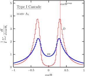
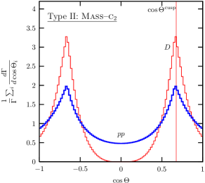
Figure 20: Normalized differential decay rates versus $\cos\Theta$ in the $D$-rest frame (thin curves) and in the $pp$ lab frame with $\sqrt{s}=14\ {\,{\rm TeV}}$ (thick curves).

In order to see the longitudinal boost effects, we convert the $\cos\Theta$ distribution in the $D$ rest frame into the $pp$ frame at the LHC, by convoluting with the parton distribution functions of a proton. In Fig. 20, we compare the summed distributions of $\cos{\Theta}_{i}$ in the $D$-rest frame (thin curves) with that in the $pp$ lab frame at $\sqrt{s}=14\ {\,{\rm TeV}}$ (thick curves). For the parton distribution function, we have used CTEQ6 cteq6 . We take the Mass–a₁ for Type I and the Mass–c₂ for Type II decay. For simplicity we assume that the heavy particle $D$ is singly produced through the $s$-channel gluon fusion and $q\bar{q}$ annihilation.

Unlike the finite width effects, the longitudinal boost effect does not completely smash the characteristic shape. The sharp cusp structures survive to some extent in both Type I and Type II cascade decays. The shift of the $\cos{\Theta}$ cusp position is minor. Moreover the overall functional shape remains the same even though the absence of events around $\cos{\Theta}=0$ in the $D$ rest frame is filled by the longitudinal boost effects. The cusp in the $\cos{\Theta}$ distribution, though Lorentz non-invariant, is quite useful to draw mass information. Again we emphasize that the $e^{+}e^{-}$ linear collider does not have this unambiguity.

V.3 Spin-correlation effect

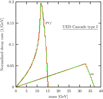
Figure 21: The $d{\Gamma}/dm$ and $d{\Gamma}/dp_{Ti}$ for the process of ${Z^{(2)}}\to\ell+{L^{(2)}}\to\ell+{B^{(1)}}{L^{(1)}}\to\ell\ell{B^{(1)}}{B^{(1)}}$ with and without spin correlations.

Our main results are based on the kinematics only, ignoring the spin-correlation in the full matrix elements. Since this paper is focused on the basic properties of the kinematic singular structures in the cascade decays, full analysis for each new physics process is beyond the scope of this paper. Nevertheless the algebraic singularity origin of the cusp and endpoint keeps them stable under the spin correlation effects Kim:2009si .

In order to demonstrate this, we consider one example, the ${Z^{(2)}}$ decay in the the UED model:

Cascade Type I: $${Z^{(2)}}\to\ell+{L^{(2)}}\to\ell+{B^{(1)}}{L^{(1)}}\to\ell\ell{B^{(1)}}{B^{(1)}}.$$ (40)

In Fig. 21, we show their spin correlation effects. We found that the spin correlations do not change the $m$ and $p_{Ti}$ distributions. Two distributions with and without spin-correlation effects are almost identical.

VI Summary and Conclusions

We have studied the singularity structure, such as cusps and endpoints, in the kinematic distributions of three-step cascade decay of a new parity-even particle $D$ and the determination of the missing particle mass by using such singularities.

Two non-trivial decay topologies, called the Type I and Type II cascade decays, have been studied. In the Type I decay ($D\to a_{1}C,~{}C\to X_{1}B,~{}B\to a_{2}X_{2}$), where the first missing particle $X_{1}$ is from the second-step decay, the distribution of the invariant mass $m$ of two visible particles, $a_{1}$ and $a_{2}$, develops a cusp. Full functional form of the $m$ distribution for general mass parameters has been derived. If the mother particle $D$ is produced at rest in the transverse direction, various longitudinal-boost invariant observables accommodate cusp structures. First there is a cusp in the transverse mass $m_{T}$ distribution, which is complementary for the $m$ cusp since the $m_{T}$ cusp shape is sharp even when the $m$ cusp is dull. Although the transverse momentum distribution of the c.m. system of two visible particles does not develop a visible cusp structure and a sharp endpoint, we note that the transverse momentum distribution of the far visible particle $a_{2}$ has a cusp, and that of the near visible particle $a_{1}$ has an endpoint of the shape of a steep cliff. We also study the summed distribution of $\cos{\Theta}_{i}$, which has two independent cusp structures.

	Antler	Cascade
		Type I	Type II
$m$	yes	yes	no
$m_{T}$	no	yes	yes
$p_{T}$	no	no	no
$p_{Tn}$	yes	no	yes
$p_{Tf}$		yes	no
$\cos\Theta$	yes	yes	yes

Table 3: The presence or absence of the cusp in the kinematic distributions of $m$, $m_{T}$, $p_{T}$, $p_{Ti}$, $\cos\Theta$ of the antler, Type I cascade, Type II cascade decays.

In the Type II decay ($D\to X_{1}C,~{}C\to a_{1}B,~{}B\to a_{2}X_{2}$), the first missing particle $X_{1}$ is from the first step decay. The kinematics of the two visible $a_{1}$ and $a_{2}$ is determined solely by the two-step cascade decay from the first intermediate particle $C$, so that the invariant mass distribution does not have a cusp structure. However, the kinematic distributions regarding the transverse motion from production of both $X_{1}$ and $X_{2}$ can carry the information from the whole three-step cascade decay. We show both the $m_{T}$ and $\sum_{i}p_{Ti}$ distributions have distinctive cusp structures. In the individual transverse momentum distribution, only the near visible particle has both a sharp cusp and a fast-falling endpoint. The $\cos{\Theta}$ distribution also shows a cusp as well. Including the antler decay topology, we have summarized the existence of cusp in the kinematic distributions of $m$, $m_{T}$, $p_{T}$, $p_{Ti}$, $\cos\Theta$ in Table 3.

We have also considered the effects of finite decay widths, longitudinal-boost of the parent particle $D$, and spin correlation. The effects of the finite widths of the intermediate particles can be significant if the decay width is sizable, say ${\Gamma}/M\mathrel{\mathop{\kern 0.0pt\hbox to0.0pt{\raise 0.86108pt\hbox{$>$}\hss}}\lower 3.87495pt\hbox{\kern-1.90002pt$\sim$}}10\%$. As the decay width increases, the sharp cusp gets smeared, and the endpoint position gets shifted to $m_{D}-2m_{X}$: the missing particle mass $m_{X}$ can be still extracted by a proper fitting. The longitudinal motion of the parent particle $D$ affects the distribution of $\cos{\Theta}$. At least for the sample mass parameters, however, the $\cos{\Theta}$ cusp remains sharp after convoluting with the parton distribution functions of a proton at the LHC. Spin correlation effects from full $S$-matrix elements turn out to be negligible in most cases, which is expected since the singularities are determined by the kinematic relations.

With the companion paper on the detailed study of the kinematic cusps in the antler decay long:antler , our analysis shows the general kinematic properties and provides useful formulae for the decay topologies with two visible particles and two missing particles. By looking at the singularity structures of various kinematic distributions, the hidden nature of the missing particle can be probed effectively and elegantly. With the outstanding performance of the LHC and detectors, this is an exciting time for such investigation.

Appendix A Invariant mass distributions for the general Type I case

In this appendix, we present the invariant mass distribution in the general Type I cascade decays:

$$D(P)\longrightarrow C+a_{1}(k_{1}),$$

$$C\longrightarrow B+X_{1},$$

$$\hskip 34.0ptB\longrightarrow a_{2}(k_{2})+X_{2}.$$

As discussed in the main text, the Type II cascade decay is practically a three body decay in the view point of visible particles. This four-body decay has generally seven different mass parameters. We define the rapidities of six particles as

$$\cosh\xi_{C} = \frac{m_{D}^{2}+m_{C}^{2}-m_{a_{1}}^{2}}{2m_{D}m_{C}},\qquad\cosh\xi_{a_{1}}=\frac{m_{D}^{2}+m_{a_{1}}^{2}-m_{C}^{2}}{2m_{D}m_{a_{1}}},$$ (42)

$${}\cosh\xi_{B} = \frac{m_{C}^{2}+m_{B}^{2}-m_{X_{1}}^{2}}{2m_{C}m_{B}},\qquad\cosh\xi_{X_{1}}=\frac{m_{C}^{2}+m_{X_{1}}^{2}-m_{B}^{2}}{2m_{C}m_{X_{1}}},$$

$${}\cosh\xi_{a_{2}} = \frac{m_{B}^{2}+m_{a_{2}}^{2}-m_{X_{2}}^{2}}{2m_{B}m_{a_{2}}},\qquad\cosh\xi_{X_{2}}=\frac{m_{B}^{2}+m_{X_{2}}^{2}-m_{a_{2}}^{2}}{2m_{B}m_{X_{2}}}.$$

A very useful kinematic variable is $\chi$, the rapidity of the particle $a_{2}$ in the rest frame of $a_{1}$:

$$\chi\equiv\cosh\xi^{(a_{1})}_{a_{2}}=\frac{m^{2}-m_{a_{1}}^{2}-m_{a_{2}}^{2}}{2m_{a_{1}}m_{a_{2}}},$$ (43)

where the superscript $(a_{1})$ denotes that the rapidity is defined in the rest frame of $a_{1}$.

The functional expression of $d\Gamma/dm$ is different according to the mass relations. The derivation of $d\Gamma/dm$ is similar to that presented in the appendix of Ref. long:antler . For simple presentation, we introduce

$$\xi_{++} = \xi_{B}+\xi_{a_{1}}+\xi_{a_{2}}+\xi_{C},$$ (44)

$$\xi_{+-} = |\xi_{B}+\xi_{a_{1}}-\xi_{a_{2}}-\xi_{C}|,$$ (45)

$$\xi_{-+} = |\xi_{B}-\xi_{a_{1}}+\xi_{a_{2}}+\xi_{C}|,$$ (46)

$$\xi_{--} = |\xi_{B}-\xi_{a_{1}}-\xi_{a_{2}}-\xi_{C}|.$$ (47)

We order $\xi_{+-}$, $\xi_{-+}$ and $\xi_{--}$ and name them $\xi_{1}\leq\xi_{2}\leq\xi_{3}$. Analytic functions forms of ${d\Gamma}/{d\chi}$ are then written as

• if $|\xi_{B}-\xi_{a_{2}}-\xi_{C}|\geq\xi_{a_{1}}$ or $\xi_{B}+\xi_{a_{2}}+\xi_{C}\leq\xi_{a_{1}}$,

  $$\frac{d\Gamma}{d\chi}\propto\begin{cases}\begin{array}[]{ll}-\xi_{1}+\cosh^{-1}\chi,&\mbox{ if $\cosh\xi_{1}\leq\chi\leq\cosh\xi_{2}$, }\\ \xi_{2}-\xi_{1},&\mbox{ if $\cosh\xi_{2}\leq\chi\leq\cosh\xi_{3}$, }\\ \xi_{++}-\cosh^{-1}\chi,&\mbox{ if $\cosh\xi_{3}\leq\chi\leq\cosh\xi_{++}$, }\\ 0,&\mbox{ otherwise.}\end{array}\end{cases}$$ (48)

• if $|\xi_{B}-\xi_{a_{2}}-\xi_{C}|<\xi_{a_{1}}<\xi_{B}+\xi_{a_{2}}+\xi_{C}$,

  $$\frac{d\Gamma}{d\chi}\propto\begin{cases}\begin{array}[]{ll}2\cosh^{-1}\chi,&\mbox{ if $1\leq\chi\leq\cosh\xi_{1}$, }\\ \xi_{1}+\cosh^{-1}\chi,&\mbox{ if $\cosh\xi_{1}\leq\chi\leq\cosh\xi_{2}$, }\\ \xi_{1}+\xi_{2},&\mbox{ if $\cosh\xi_{2}\leq\chi\leq\cosh\xi_{3}$, }\\ \xi_{++}-\cosh^{-1}\chi,&\mbox{ if $\cosh\xi_{3}\leq\chi\leq\cosh\xi_{++}$, }\\ 0,&\mbox{ otherwise.}\end{array}\end{cases}$$ (49)

The positions of the minimum, cusp, and maximum of the invariant mass distribution are

$$M^{\rm min}_{\rm cas1} = \left\{\begin{array}[]{ll}\sqrt{m_{a_{1}}^{2}+m_{a_{2}}^{2}+2m_{a_{1}}m_{a_{2}}\cosh\xi_{1}},&\hbox{ for }\mathcal{R}_{1,\cdots,6}\\ m_{a_{1}}+m_{a_{2}},&\hbox{ for }\mathcal{R}_{7,\cdots,12}\\ \end{array}\right.$$ (52)

$${}M^{\rm cusp}_{\rm cas1} = \sqrt{m_{a_{1}}^{2}+m_{a_{2}}^{2}+2m_{a_{1}}m_{a_{2}}\cosh\xi_{3}},$$

$${}M^{\rm max}_{\rm cas1} = \sqrt{m_{a_{1}}^{2}+m_{a_{2}}^{2}+2m_{a_{1}}m_{a_{2}}\cosh\xi_{++}}.$$

References

- (1) S. Perlmutter et al., Astrophys. J. 517, 565-586 (1999); A. G. Riess et al., Astron. J. 116, 1009-1038 (1998); A. G. Riess, R. P. Kirshner, B. P. Schmidt et al., Astron. J. 117, 707-724 (1999).
- (2) E. J. Copeland, M. Sami, S. Tsujikawa, Int. J. Mod. Phys. D15, 1753-1936 (2006); L. M. Krauss, M. S. Turner, Gen. Rel. Grav. 27, 1137-1144 (1995).
- (3) G. Bertone, D. Hooper and J. Silk, Phys. Rept. 405, 279 (2005).
- (4) A. Djouadi, Phys. Rept. 459, 1 (2008); G. Jungman, M. Kamionkowski and K. Griest, Phys. Rept. 267, 195 (1996).
- (5) G. Servant and T. M. P. Tait, Nucl. Phys. B 650, 391 (2003); F. Burnell and G. D. Kribs, Phys. Rev. D 73, 015001 (2006); K. Kong and K. T. Matchev, JHEP 0601, 038 (2006).
- (6) I. Low, JHEP 0410, 067 (2004); A. Birkedal, A. Noble, M. Perelstein and A. Spray, Phys. Rev. D 74, 035002 (2006); J. Hubisz and P. Meade, Phys. Rev. D 71, 035016 (2005); A. Freitas, P. Schwaller and D. Wyler, JHEP 0912, 027 (2009) [Erratum-ibid. 1102, 032 (2011)].
- (7) M. Burns, K. Kong, K. T. Matchev and M. Park, JHEP 0903, 143 (2009).
- (8) I. Hinchliffe, F. E. Paige, M. D. Shapiro, J. Soderqvist and W. Yao, Phys. Rev. D 55, 5520 (1997); H. Bachacou, I. Hinchliffe and F. E. Paige, Phys. Rev. D 62, 015009 (2000); B. C. Allanach, C. G. Lester, M. A. Parker and B. R. Webber, JHEP 0009, 004 (2000); B. K. Gjelsten, D. J. Miller and P. Osland, JHEP 0412, 003 (2004); B. K. Gjelsten, D. J. Miller and P. Osland, JHEP 0506, 015 (2005).
- (9) M. M. Nojiri, G. Polesello and D. R. Tovey, arXiv:hep-ph/0312317. K. Kawagoe, M. M. Nojiri and G. Polesello, Phys. Rev. D 71, 035008 (2005).
- (10) H. C. Cheng, J. F. Gunion, Z. Han, G. Marandella and B. McElrath, JHEP 0712, 076 (2007); M. M. Nojiri and M. Takeuchi, JHEP 0810, 025 (2008); H. C. Cheng, D. Engelhardt, J. F. Gunion, Z. Han and B. McElrath, Phys. Rev. Lett. 100, 252001 (2008).
- (11) C. G. Lester and D. J. Summers, Phys. Lett. B 463, 99 (1999).
- (12) A. Barr, C. Lester and P. Stephens, J. Phys. G 29, 2343 (2003); P. Meade and M. Reece, Phys. Rev. D 74, 015010 (2006); S. Matsumoto, M. M. Nojiri and D. Nomura, Phys. Rev. D 75, 055006 (2007); C. Lester and A. Barr, JHEP 0712, 102 (2007).
- (13) W. S. Cho, K. Choi, Y. G. Kim and C. B. Park, Phys. Rev. Lett. 100, 171801 (2008); B. Gripaios, JHEP 0802, 053 (2008); A. J. Barr, B. Gripaios and C. G. Lester, JHEP 0802, 014 (2008); W. S. Cho, K. Choi, Y. G. Kim and C. B. Park, JHEP 0802, 035 (2008); M. M. Nojiri, Y. Shimizu, S. Okada and K. Kawagoe, JHEP 0806, 035 (2008).
- (14) M. Serna, JHEP 0806, 004 (2008); M. M. Nojiri, K. Sakurai, Y. Shimizu and M. Takeuchi, JHEP 0810, 100 (2008).
- (15) T. Han, I. W. Kim and J. Song, Phys. Lett. B 693, 575 (2010).
- (16) T. Han, I. W. Kim and J. Song, arXiv:1206.5633 [hep-ph].
- (17) K. Agashe, D. Kim, M. Toharia and D. G. E. Walker, Phys. Rev. D 82, 015007 (2010); W. S. Cho, D. Kim, K. T. Matchev and M. Park, arXiv:1206.1546 [hep-ph].
- (18) A. Datta, K. Kong and K. T. Matchev, Phys. Rev. D 72, 096006 (2005) [Erratum-ibid. D 72, 119901 (2005)]; H. C. Cheng, K. T. Matchev and M. Schmaltz, Phys. Rev. D 66, 036005 (2002).
- (19) H. C. Cheng, K. T. Matchev and M. Schmaltz, Phys. Rev. D 66, 036005 (2002). ,
- (20) T. Appelquist and H. U. Yee, Phys. Rev. D 67, 055002 (2003).
- (21) T. G. Rizzo and J. D. Wells, Phys. Rev. D 61, 016007 (1999); A. Strumia, Phys. Lett. B 466, 107 (1999); C. D. Carone Phys. Rev. D 61, 015008 (1999); I. Gogoladze and C. Macesanu Phys. Rev. D 74, 093012 (2006).
- (22) P. Nath and M. Yamaguchi, Phys. Rev. D 60, 116006 (1999); K. Agashe, N. G. Deshpande, and G. H. Wu Phys. Lett. B 511, 85 (2001).
- (23) D. Chakraverty, K. Huiti, and A. Kundu, Phys. Lett. B 558, 173 (2003); A. J. Buras, M. Spranger, and A. Weiler Nucl. Phys. B 660, 225 (2003); A. J. Buras, A. Poschenrieder, M. Spranger, and A. Weiler Nucl. Phys. B 678, 455 (2004); K. Agashe, N. G. Deshpande, and G. H. Wu, Phys. Lett. B 514, 309 (2001).
- (24) B. Abbott et al., D0 Collaboration, Phys. Rev. Lett. 83, 4937 (1999).
- (25) I. Hinchliffe, F. E. Paige, M. D. Shapiro, J. Soderqvist and W. Yao, Phys. Rev. D 55, 5520 (1997); H. Bachacou, I. Hinchliffe and F. E. Paige, Phys. Rev. D 62, 015009 (2000)
- (26) S. Kretzer, H. L. Lai, F. I. Olness, W. K. Tung, Phys. Rev. D69, 114005 (2004).
- (27) I. W. Kim, Phys. Rev. Lett. 104, 081601 (2010).