What You Can Do with Coordinated Samples

Abstract

Sample coordination, where similar instances have similar samples, was proposed by statisticians four decades ago as a way to maximize overlap in repeated surveys. Coordinated sampling had been since used for summarizing massive data sets.

The usefulness of a sampling scheme hinges on the scope and accuracy within which queries posed over the original data can be answered from the sample. We aim here to gain a fundamental understanding of the limits and potential of coordination. Our main result is a precise characterization, in terms of simple properties of the estimated function, of queries for which estimators with desirable properties exist. We consider unbiasedness, nonnegativity, finite variance, and bounded estimates.

Since generally a single estimator can not be optimal (minimize variance simultaneously) for all data, we propose variance competitiveness, which means that the expectation of the square on any data is not too far from the minimum one possible for the data. Surprisingly perhaps, we show how to construct, for any function for which an unbiased nonnegative estimator exists, a variance competitive estimator.

1 Introduction

Many data sources, including IP or Web traffic logs from different time periods or locations, measurement data, snapshots of data depositories that evolve over time, and document/feature and market-basket data, can be viewed as a collection of instances, where each instance is an assignment of numeric values from some set $V$ to a set of items (the set of items is the same for different instances but the value of each item changes).

When the data is too massive to manipulate or even store in full, it is useful to obtain and work with a random sample of each instance. Two common sampling schemes are Poisson sampling (each item is sampled independently with probability that depends only on its value) and bottom-$k$ (order) sampling. The samples are efficient to compute, also when instances are presented as streams or are distributed across multiple servers. It is convenient to specify these sampling schemes through a rank function, $r:[0,1]\times V\rightarrow\mathbb{R}$, which maps seed-value pairs to a number $r(u,v)$ that is non-increasing with $u$ and non-decreasing with $v$. For each item $h$ we draw a seed $u(h)\sim U[0,1]$ uniformly at random and compute the rank value $r(u(h),v(h))$, where $v(h)$ is the value of $h$. With Poisson sampling, item $h$ is sampled $\iff$ $r(u(h),v(h))\geq T(h)$, where $T(h)$ are fixed thresholds, whereas a bottom-$k$ sample includes the $k$ items with highest ranks. Poisson PPS samples (Probability Proportional to Size [26], where each item is included with probability proportion to its value) are obtained using the rank function $r(u,v)=v/u$ and a fixed $T(h)$ across items. Priority (sequential Poisson) samples [33, 20, 38] are bottom-$k$ samples utilizing the PPS ranks $r(u,v)=v/u$ and successive weighted sampling without replacement  [35, 21, 11] corresponds to bottom-$k$ samples with the rank function $r(u,v)=-v/\ln(u)$.

Samples of different instances are coordinated when the set of random seeds $u(h)$ is shared across instances. Scalable sharing of seeds when instances are dispersed in time or location is facilitated through random hash functions $u(h)\leftarrow H(h)$, where the only requirement for our purposes is uniformity and pairwise independence. Figure 1 contains an example data set of two instances and the PPS sampling probabilities of each item in each instance, and illustrates how to coordinate the samples. Note that the sample of one instance does not depend on values assumed in other instances, which is important for scalable deployment.

Why coordinate samples? Sample coordination was proposed in 1972 by Brewer, Early, and Joice [3], as a method to maximize overlap and therefore minimize overhead in repeated surveys [37, 34, 36]: The values of items change, and therefore there is a new set of PPS sampling probabilities. With coordination, the sample of the new instance is as similar as possible to the previous sample, and therefore the number of items that need to be surveyed again is minimized. Coordination was subsequently used to facilitate efficient processing of large data sets. Coordinated samples of instances are used as synopses which facilitate efficient estimation of multi-instance functions such as distinct counts (cardinality of set unions), sum of maxima, and similarity [5, 4, 7, 18, 31, 22, 23, 6, 19, 12, 2, 25, 13, 17]. Estimates obtained over coordinated samples are much more accurate than possible with independent samples. Used this way, coordinated sampling can be casted as a form of Locality Sensitive Hashing (LSH) [29, 24, 28]. Lastly, coordinated samples can sometimes be obtained much more efficiently than independent samples. One example is computing samples of the $d$-neighborhoods of all nodes in a graph [7, 10, 31, 11, 12, 8]. Similarity queries between neighborhoods are useful in the analysis of massive graph datasets such as social networks or Web graphs.

Our aim here is to study the potential and limitations of estimating multi-instance functions from coordinated samples of instances. The same set of samples can be used to estimate multiple queries, including queries that are specified only after sampling is performed. The sample may also be primarily used ro estimate subset statistics over one instance as a time, such as sums, averages, and moments. While we focus here on queries that span multiple instances, we keep this in mind, and therefore do not aim for a sampling scheme optimized for a particular query (although some of our results can be applied this way), but rather, to optimize the estimator given the sampling scheme and query.

items:	1	2	3	4	5	6	7	8
Instance1:	1	0	4	1	0	2	3	1
Instance2:	3	2	1	0	2	3	1	0
PPS sampling probabilities for T=4 (sample of expected size 3):
Instance1:	0.25	0.00	1.00	0.25	0.00	0.50	0.75	0.25
Instance2:	0.75	0.50	0.25	0.00	0.50	0.75	0.25	0.00

Figure 1: Two instances with 8 items and respective PPS sampling probabilities for threshold value $4$, so item with value $v$ is sampled with probability $\min\{1,v/4\}$. To obtain two coordinated PPS samples of the instances, we associate an independent $u(i)\sim U[0,1]$ with each item $i\in[8]$. We then sample $i\in[8]$ in instance $h\in[2]$ if and only if $u(i)\leq v_{h}(i)/4$, where $v_{h}(i)$ is the value of $i$ in instance $h$. When coordinating the samples this way, we make them as similar as possible. In the example, item $1$ will always (for any drawing of seeds) be sampled in instance $2$ if it is sampled in instance $1$ and vice versa for item $7$.

Sum aggregates: Most queries in the above examples can be casted as sum aggregates over selected items $h$ of an item function $f(\boldsymbol{v})$ applied to the item weight tuple in different instances $\boldsymbol{v}(h)=(v_{1}(h),v_{2}(h),\cdots)$. In particular, distinct count (set union) is a sum aggregate of $OR(\boldsymbol{v})$, max-sum aggregates $\max(\boldsymbol{v})=\max_{i}v_{i}$, min-sum aggregates $\min(\boldsymbol{v})=\min_{i}v_{i}$, and $L_{p}^{p}$ ($p$th power of L_p-difference) is the sum aggregate of the exponentiated range function $\mbox{{\sc rg}}_{p}(\boldsymbol{v})=|\max(\boldsymbol{v})-\min(\boldsymbol{v})|^{p}$. In our example of Figure 1, $L_{2}^{2}$ of items $[4]$ is $(1-3)^{2}+(2-0)^{2}+(4-1)^{2}+(1-0)^{2}=18$, and is computed by summing the item function $\mbox{{\sc rg}}_{2}(v_{1},v_{2})=(v_{1}-v_{2})^{2}$ over these items. The $L_{1}$ of items $\{1,3\}$ is $|1-3|+|4-1|=5$, using the item function $\mbox{{\sc rg}}(v_{1},v_{2})=|v_{1}-v_{2}|$, and the max-sum of items $\{6,7,8\}$ is $\max\{2,3\}+\max\{3,1\}+\max\{1,0\}=7$, which uses the item function $\max\{v_{1},v_{2}\}$. Other queries in our examples which are not in sum aggregate form can be approximated well by sum aggregates: The Jaccard similarity is a ratio of min-sum and max-sum, and thus the ratio of min-sum estimate with small additive error and a max-sum estimate with small relative error [17] is a good Jaccard similarity estimator. The $L_{p}$ difference is the $p$th root of $L_{p}^{p}$, and can be estimated well by taking the $p$th root of a good estimator for $L_{p}^{p}$, which is a sum aggregate of $\mbox{{\sc rg}}_{p}$. When the domain of query results is nonnegative, as is the case in the examples, the common practice, which we follow, is to restrict the estimates, which often are plugged in instead of the exact result, to be nonnegative as well.

Sum estimators – one item at a time: To estimate a sum aggregate, we can use a linear estimator which is the sum of single-item estimators, estimating the item function $f(\boldsymbol{v}(h))$ for each selected item $h$. We refer to such an estimator as a sum estimator. When the single-item estimators are unbiased, from linearity of expectation, so is the sum estimate. When the single-item estimators are unbiased and sampling of different items is pairwise independent (respectively, negatively correlated, as with bottom-$k$ sampling), the variance of the sum is (resp., at most) the sum of variances of the single-item estimators. Therefore, the relative error of the sum estimator decreases with the number of selected items we aggregate over. We emphasize that unbiasedness of the single-item estimators (together with pairwise independence or negative correlations between items) is critical for good estimates of the sum aggregate since a variance component that is due to bias “adds up” with aggregation whereas otherwise the relative error “cancels out” with aggregation. The Horvitz-Thompson (HT) estimator [27] is a classic sum estimator which is unbiased and nonnegative. To estimate $f(v)$, the HT estimator outputs $0$ when the value is not sampled and the inverse-probability estimate $f(v)/p$ when the value is sampled, where $p$ is the sampling probability. The HT estimator is applicable to some multi-instance functions [17].

From here on, we restrict our attention to estimating item functions $f(\boldsymbol{v})\geq 0$ where each entry of $\boldsymbol{v}$ is Poisson sampled and focus on unbiased and nonnegative estimators for $f(\boldsymbol{v})$. We provide the model in detail in Section 2. See Appendix B for further discussion on using sum estimators with bottom-$k$ samples.

The challenge we address: Throughout the 40 year period in which coordination was used, estimators were developed in an ad-hoc manner, lacking a fundamental understanding of the potential and limits of the approach. Prior work was mostly based on adaptations of the HT estimator for multiple instances. The HT estimator is applicable provided that for any $\boldsymbol{v}$ where $f(\boldsymbol{v})>0$, there is a positive probability for an outcome that both reveals $f(\boldsymbol{v})$ and allows us to determine a probability $p$ for such an outcome. These conditions are satisfied by some basic functions including $\max(\boldsymbol{v})$ and $\min(\boldsymbol{v})$. There are functions, however, for which the HT estimator is not applicable, but nonetheless, for which nonnegative and unbiased estimators exist. Moreover, the HT estimator may not be optimal even when it is applicable.

As a particular example, the only $L_{p}$ difference for which a “satisfactory” estimator was known was the $L_{1}$ difference [17]. Stated in terms of estimators for item functions, prior to our work, there was no unbiased and nonnegative estimator known for $\mbox{{\sc rg}}_{p}(\boldsymbol{v})=|\max(\boldsymbol{v})-\min(\boldsymbol{v})|^{p}$ for any $p\not=1$. For $p=1$, the known estimator used the relation $\mbox{{\sc rg}}(\boldsymbol{v})=\max(\boldsymbol{v})-\min(\boldsymbol{v})$, separately estimating the maximum and the minimum and showing that when samples are coordinated then the estimate for the maximum is always at least as large as the one for the minimum and therefore the difference of the estimates is never negative. But even for this $\mbox{{\sc rg}}(\boldsymbol{v})$ estimator, there was no understanding whether it is “optimal” and more so, what optimality even means in this context. Moreover, the ad hoc construction of this estimator does not extend even to slight variations, like $\max\{v_{1}-v_{2},0\}$, which sum-aggregates to the natural “one sided” $L_{1}$ difference.

Contributions highlights

Characterization: We provide a complete characterization, in terms of simple properties of the function $f$ and the sampling scheme parameters, of when estimators with the following combinations of properties exist for $f$:

• $\bullet$ unbiasedness and nonnegativity.

• $\bullet$ unbiasedness, nonnegativity, and finite variances, which means that for all $\boldsymbol{v}$, the variance given data $\boldsymbol{v}$ is finite.

• $\bullet$ unbiasedness, nonnegativity, and bounded estimates, which means that for each $\boldsymbol{v}$, there is an upper bound on all estimates that can be obtained when the data is $\boldsymbol{v}$. Bounded estimates implies finite variances, but not vice versa.

The J estimator Our characterization utilizes a construction of an estimator, which we call the J estimator, which we show has the following properties: The J estimator is unbiased and nonnegative if and only if an unbiased nonnegative estimator exists for $f$. The J estimator has a finite variance for data $\boldsymbol{v}$ or is bounded for data $\boldsymbol{v}$ if and only if an (nonnegative unbiased) estimator with the respective property for $\boldsymbol{v}$ exists.

Variance competitiveness: Ideally, we would like to have a single estimator, which subject to desired properties of the estimator, minimizes the variance for all data. Such estimators are known in the statistics literature as UMVUE (uniform minimum variance unbiased) estimators [32]. Generally however, an (unbiased, nonnegative, linear) estimator with minimum variance on all data vectors [30] may not exist. Simple examples show that this is also the case for our coordinated sampling model even when restricting our attention to particular natural functions.

We are therefore introducing and aiming for a notion of variance competitiveness, which means that for any data vector, the variance of our estimator is not “too far” from the minimum variance possible for that vector by a nonnegative unbiased estimator. More precisely, an estimator is $c$-competitive if for all data $\boldsymbol{v}$, the expectation of its square is within a factor of $c$ from the minimum possible for $\boldsymbol{v}$ by an estimator that is unbiased and nonnegative on all data. Variance competitiveness bridges the gap between the ideal UMVUE estimators (which generally do not exist) and the practice of estimator selections with no “worst-case” guarantees.

$\boldsymbol{v}$-optimality: To study competitiveness, we need to compare the variance on each data vector to the minimum possible, and to do so, we need to be able to express the “best possible” estimates. We say that an estimator is $\boldsymbol{v}$-optimal if amongst all estimators that are unbiased and nonnegative on all data, it minimizes variance for the data $\boldsymbol{v}$. We express the $\boldsymbol{v}$-optimal estimates, which are the values a $\boldsymbol{v}$-optimal estimator assumes on outcomes that are consistent with data $\boldsymbol{v}$, and the respective $\boldsymbol{v}$-optimal variance. We show that the $\boldsymbol{v}$-optimal estimates are uniquely defined (almost everywhere). The $\boldsymbol{v}$-optimal estimates, however, are inconsistent for different data since as we mentioned earlier, it is not generally possible to obtain a single unbiased nonnegative estimator that minimizes variance for all data vectors. They do allow us, however, to analyse the competitiveness of estimators, and in particular, that of the J estimator.

Competitiveness of the J estimator: We show that the J estimator is competitive. In particular, this shows the powerful and perhaps surprising result that whenever for any particular data vector $\boldsymbol{v}$ there exists an estimator with finite variance that is nonnegative and unbiased on all data, then there is a single estimator, that for all data, has expectation of the square that is $O(1)$ of the minimum possible.

2 Coordinated Shared-Seed Sampling for a Single Item

Using the terminology in the introduction, we are now looking at a single item, its values $\boldsymbol{v}=(v_{1},\ldots,v_{r})$ in different instances, the sampling scheme projected on this one item, and estimating the item function $f$.

We denote that data domain by ${\bf V}\subseteq\mathbb{R}^{r}_{\geq 0}$. The sampling scheme is specified by non-decreasing continuous functions $\mbox{\boldmath{$\tau$}}=(\tau_{1},\ldots,\tau_{r})$ on $[0,1]$ such that the infimum of the range of $\tau_{i}$ is at most $\inf_{\boldsymbol{v}\in{\bf V}}v_{i}$.

The sampling of $\boldsymbol{v}$ is performed by drawing a random value $u\sim U[0,1]$, which we refer to as the seed. We then include the $i$th entry in the outcome $S$ if and only if $v_{i}$ is at least $\tau_{i}(u)$:

$$i\in S\,\iff\,v_{i}\geq\tau_{i}(u)\ .$$

We use the notation $S(u,\boldsymbol{v})$ for the outcome of the sampling scheme applied to data $\boldsymbol{v}$ and seed $u$.

Sampling is PPS if $\tau_{i}(u)$ are linear functions: there is a fixed vector $\tau^{*}$ such that $\tau_{i}(u)\equiv u\tau^{*}_{i}$, in which case entry $i$ is included with probability $\min\{1,v_{i}/\tau^{*}_{i}\}$. Our use of the term PPS in this single-item context is compatible with PPS sampling of each instance $i$ using threshold $\tau^{*}_{i}$. In this case, we look at the “projected” sampling scheme on the $i$th entry of our item’s tuple.

Observe that our model assumes weighted sampling, where the probability that an entry is sampled depends (and is non-decreasing) with its value. Transiting briefly back to sampling of instances, weighted sampling results in more accurate estimation of quantities (such as averages of sums) where larger values contribute more. It is also important for boolean domains (${\bf V}=\{0,1\}^{r}$) when most items have $0$ values and in this case, enables us to sample only “active” items.

We assume that the seed $u$ and the functions $\tau$ are available to the estimator, and in particular, treat the seed as provided with the outcome. When an entry is sampled, we know its value and also can compute the probability that it is sampled. When an entry is not sampled, we know that its value is at most $\tau_{i}(u)$ and we can compute this upper bound from the seed $u$ and the function $\tau_{i}$. Putting this information together, for each outcome $S(u,\boldsymbol{v})$, we can define the set $V^{*}(S)$ of all data vectors consistent with the outcome. This set captures all the information we can glean from the sample on the data.

$$V^{*}(S)\equiv V^{*}(u,\boldsymbol{v})=\{\boldsymbol{z}\mid\forall i\in[r],\left(i\in S\wedge z_{i}=v_{i}\right)\,\vee\,\left(i\not\in S\wedge z_{i}<\tau_{i}(u)\right)\}\ .$$

Structure of the set of outcomes. From the outcome, which is the set of sampled entries and the seed $\rho$, we can determine $V^{*}(u,\boldsymbol{v})$ also for all $u\geq\rho$. We also have that for all $u\geq\rho$ and $\boldsymbol{z}\in V^{*}(\rho,v)$, $V^{*}(u,\boldsymbol{z})=V^{*}(u,\boldsymbol{v})$. Fixing $\boldsymbol{v}$, the sets $V^{*}(u,\boldsymbol{v})$ are non-decreasing with $u$ and the set $S$ of sampled entries is non-increasing, meaning that $V^{*}(u,\boldsymbol{v})\subset V^{*}(\rho,\boldsymbol{v})$ and $S(u,\boldsymbol{v})\supset S(\rho,\boldsymbol{v})$ when $u<\rho$.

The containment order of the sets $V^{*}(S)$ is a tree-like partial order on outcomes. For two outcomes, the sets $V^{*}(S)$ are either disjoint, and unrelated in the containment order, or one is fully contained in another, and succeeds it in the containment order. The outcome $S(u,\boldsymbol{v})$ precedes $S(\rho,\boldsymbol{v})$ in the containment order if and only if $u>\rho$. When $V$ is finite, the containment order is a tree order, as shown in Figure 2.

Figure 2: Illustration of the containment order on all possible outcomes $V^{*}(S)$. Example has data domain ${\bf V}=\{0,1,2\}\times\{0,1,2\}$ and seed mappings $\tau_{1}=\tau_{2}\equiv\tau$. The root of the tree corresponds to outcomes with $u\in(\tau^{-1}(2),1]$. In this case, the outcome reveals no information on the data and $V^{*}(S)$ contains all vectors in ${\bf V}$. When $u\in(\tau^{-1}(1),\tau^{-1}(2)]$ the outcome identifies entries in the data that are equal to “2”. When $u\in(0,\tau^{-1}(1)]$, the outcome reveals the data vector.

For $\boldsymbol{z}$ and $\boldsymbol{v}$, the set of all $u$ such that $\boldsymbol{z}\in S(u,\boldsymbol{v})$, if not empty, is a suffix of $(0,1]$ that is open to the left.

Lemma 2.1

$$\forall\rho\in(0,1]\ \forall\boldsymbol{v}$$

$$\boldsymbol{z}\in V^{*}(\rho,\boldsymbol{v})\implies\exists\epsilon>0,\ \forall x\in(\rho-\epsilon,1],\ \boldsymbol{z}\in V^{*}(x,\boldsymbol{v})$$

Proof

Correctness for all $x\in[\rho,1]$ follows from the structure of the set of outcomes: Since $V^{*}(x,\boldsymbol{v})\supset V^{*}(\rho,\boldsymbol{v})$ for all $x\geq\rho$ then $\boldsymbol{z}\in V^{*}(\rho,\boldsymbol{v})\implies\boldsymbol{z}\in V^{*}(x,\boldsymbol{v})$.

Consider now the set $S$ of entries that satisfy $v_{i}\geq\tau_{i}(\rho)$. Since $\boldsymbol{z}\in V^{*}(\rho,\boldsymbol{v})$, we have $\forall i\in S,z_{i}=v_{i}$ and $\forall i\not\in S,\ \max\{z_{i},v_{i}\}<\tau_{i}(\rho)$. Since $\tau_{i}$ is continuous and monotone, for all $i\not\in S$, there must be an $\epsilon_{i}>0$ such that $\tau_{i}(\rho-\epsilon_{i})>\max\{z_{i},v_{i}\}$. We now take $\epsilon=\min_{i\not\in S}\epsilon_{i}$ to conclude the proof.  
 

3 Estimators and properties

Let $f:{\bf V}$ be a function mapping ${\bf V}$ to the nonnegative reals. An estimator $\hat{f}$ of $f$ is a numeric function applied to the outcome. We use the notation $\hat{f}(u,\boldsymbol{v})\equiv\hat{f}(S(u,\boldsymbol{v}))$. On continuous domains, an estimator must be (Lebesgue) integrable. An estimator is fully specified for $\boldsymbol{v}$ if specified on a set of outcomes that have probability $1$ given data $\boldsymbol{v}$. Two estimators $\hat{f}_{1}$ and $\hat{f}_{2}$ are equivalent if for all data $\boldsymbol{v}$, $\hat{f}_{1}(u,\boldsymbol{v})=\hat{f}_{2}(u,\boldsymbol{v})$ with probability $1$.

An estimator $\hat{f}$ is nonnegative if $\forall S,\ \hat{f}(S)\geq 0$ and is unbiased if $\forall\boldsymbol{v},\ {\textsf{E}}[{\hat{f}}|\boldsymbol{v}]=f(\boldsymbol{v})$. An estimator has finite variance on $\boldsymbol{v}$ if $\int_{0}^{1}\hat{f}(u,\boldsymbol{v})^{2}du<\infty$ (the expectation of the square is finite) and is bounded on $\boldsymbol{v}$ if $\sup_{u\in(0,1]}\hat{f}(u,\boldsymbol{v})<\infty$. If a nonnegative estimator is bounded on $\boldsymbol{v}$, it also has finite variance for $\boldsymbol{v}$. We say that an estimator is bounded or has finite variances if the respective property holds for all $\boldsymbol{v}\in{\bf V}$.

$\boldsymbol{v}$-optimality. We say that an unbiased and nonnegative estimator is $\boldsymbol{v}$-optimal, that is, optimal with respect to a data vector $\boldsymbol{v}$, if it has minimum variance for $\boldsymbol{v}$. We refer to the estimates that a $\boldsymbol{v}$-optimal estimator assumes on outcomes consistent on data $\boldsymbol{v}$ as the $\boldsymbol{v}$-optimal estimates and to the minimum variance attainable for $\boldsymbol{v}$ as the $\boldsymbol{v}$-optimal variance.

Variance competitiveness. An estimator $\hat{f}$ is $c$-competitive if

$$\forall\boldsymbol{v},\,\int_{0}^{1}\bigg{(}\hat{f}(u,\boldsymbol{v})\bigg{)}^{2}du\leq c\inf_{\hat{f}^{\prime}}\int_{0}^{1}\bigg{(}\hat{f}^{\prime}(u,\boldsymbol{v})\bigg{)}^{2}du,$$

where the infimum is over all unbiased nonnegative estimators $\hat{f}^{\prime}$ of $f$. For any unbiased estimator, the expectation of the square is closely related to the variance:

$$\mbox{\sc var}[\hat{f}|\boldsymbol{v}] =\int_{0}^{1}(\hat{f}(u,\boldsymbol{v})-f(\boldsymbol{v}))^{2}du=\int_{0}^{1}\hat{f}(u,\boldsymbol{v})^{2}du-f(\boldsymbol{v})^{2}$$ (1)

When minimizing the expectation of the square, we also minimize the variance. Moreover, $c$-competitiveness means that

$$\forall\boldsymbol{v},\ \mbox{\sc var}[\hat{f}|\boldsymbol{v}]\leq c\inf_{\hat{f}^{\prime}}\mbox{\sc var}[\hat{f}^{\prime}|\boldsymbol{v}]+(c-1)f(\boldsymbol{v})^{2}$$ (2)

for all data vectors $\boldsymbol{v}$ for which a nonnegative unbiased estimator with finite variance on $\boldsymbol{v}$ exists, the variance of the estimator is at most $c$ times the $\boldsymbol{v}$-optimal variance plus an additive term of $(c-1)$ times $f(\boldsymbol{v})^{2}$.

An important remark is due here. In the typical scenario, discussed in the introduction, the sample is likely to provide little or no information on $f(\boldsymbol{v})$, the variance is $\Omega(f(\boldsymbol{v})^{2})$, and hence competitiveness as we defined it in terms of the expectation of the square translates to competitiveness of the variance. Otherwise, when for some data in the domain the sample is likely to reveal the value, it is not possible to obtain a universal competitiveness result in terms of variance. (One such example is rg on PPS samples, looking at data tuples where the maximum has sampling probability $1$.) Interestingly, for $\mbox{{\sc rg}}_{2}$ it is possible to get a bounded ratio in terms of variance. More details are in the companion experimental paper [16].

4 The lower bound function and its lower hull

For a function $f$, we define the respective lower bound function $\underline{f}$ and the lower hull function $H_{f}$. We then characterize, in terms of properties of $\underline{f}$ and $H_{f}$ when nonnegative unbiased estimators exists for $f$ and when such estimators exist that also have finite variances or are bounded.

The lower bound function $\underline{f}(S)$: For $Z\subset{\bf V}$, we define $\underline{f}(Z)=\inf\{f(v)\mid v\in Z\}$ to be the tightest lower bound on the values of $f$ on $Z$. We use the notation $\underline{f}(S)\equiv\underline{f}(V^{*}(S))$, $\underline{f}(\rho,\boldsymbol{v})\equiv\underline{f}(V^{*}(\rho,\boldsymbol{v}))$. When $\boldsymbol{v}$ is fixed, we use $\underline{f}^{(\boldsymbol{v})}(u)\equiv\underline{f}(u,\boldsymbol{v})$.

From Lemma 2.1, we obtain that $\forall\boldsymbol{v},\ \underline{f}^{(\boldsymbol{v})}(u)$ is left-continuous, that is:

Corollary 4.1

$\forall\boldsymbol{v}\forall\rho\in(0,1],\ \lim_{\eta\rightarrow\rho^{-}}\underline{f}^{(\boldsymbol{v})}(\eta)=\underline{f}^{(\boldsymbol{v})}(\rho)$.

Lemma 4.2

A nonnegative unbiased estimator $\hat{f}$ must satisfy

$$\forall\boldsymbol{v},\forall\rho,\int_{\rho}^{1}\hat{f}(u,\boldsymbol{v})du\leq\underline{f}^{(\boldsymbol{v})}(\rho)$$ (3)

Proof

Unbiased and nonnegative $\hat{f}$ must satisfy

$$\forall\boldsymbol{v},\forall\rho\in(0,1].\ \int_{\rho}^{1}\hat{f}(u,\boldsymbol{v})du\leq\int_{0}^{1}\hat{f}(u,\boldsymbol{v})du=f(\boldsymbol{v})\ .$$ (4)

From definition of $\underline{f}$, for all $\epsilon>0$ and $\rho$, there is a vector ${\boldsymbol{z}}^{(\epsilon)}\in S(\rho,\boldsymbol{v})$ such that $f(\boldsymbol{z}^{(\epsilon)})\leq\underline{f}(\rho,\boldsymbol{v})+\epsilon$. Recall that for all $u\geq\rho$, $S(u,\boldsymbol{v})=S(u,\boldsymbol{z}^{(\epsilon)})$, hence, using, (4),

$$\int_{\rho}^{1}\hat{f}(u,\boldsymbol{v})du=\int_{\rho}^{1}\hat{f}(u,\boldsymbol{z}^{(\epsilon)})du\leq f(\boldsymbol{z}^{(\epsilon)})\leq\underline{f}(\rho,\boldsymbol{v})+\epsilon\ .$$

Taking the limit as $\epsilon\rightarrow 0$ we obtain $\int_{\rho}^{1}\hat{f}(u,\boldsymbol{v})du\leq\underline{f}(\rho,\boldsymbol{v})\ .$  
 

The lower hull of the lower bound function and $\boldsymbol{v}$-optimality: We denote the function corresponding to the lower boundary of the convex hull (lower hull) of $\underline{f}^{(\boldsymbol{v})}$ by $H^{(\boldsymbol{v})}_{f}$. Our interest in the lower hull is due to the following relation (The proof is postponed to Section A):

Theorem 4.1

An estimator $\hat{f}$ is $\boldsymbol{v}$-optimal if and only if for $u\in[0,1]$ almost everywhere

$$\hat{f}(u,\boldsymbol{v})=-\frac{dH^{(\boldsymbol{v})}_{f}(u)}{du}\ .$$

Moreover, when an unbiased and nonnegative estimator exists for $f$, there also exists, for any data $\boldsymbol{v}$, a nonnegative and unbiased $\boldsymbol{v}$-optimal estimator.

We use the notation $\hat{f}^{(\boldsymbol{v})}(u)=-\frac{dH^{(\boldsymbol{v})}_{f}(u)}{du}$ for the $\boldsymbol{v}$-optimal estimates on outcomes consistent with $\boldsymbol{v}$. Since the lower bound function is monotone non-increasing, so is $H^{(\boldsymbol{v})}_{f}$, and therefore $H^{(\boldsymbol{v})}_{f}$ is differentiable almost everywhere and $\hat{f}^{(\boldsymbol{v})}$ is defined almost everywhere. Figure 3 illustrates an example lower bound function and the corresponding lower hull.

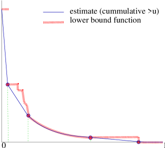
Figure 3: Lower bound function $\underline{f}^{(\boldsymbol{v})}(u)$ for $u\in(0,1]$ and corresponding lower hull $H^{(\boldsymbol{v})}_{f}(u)$, which is also the integral of the nonnegative estimator with minimum variance on $\boldsymbol{v}$: $\int_{u}^{1}\hat{f}^{(\boldsymbol{v})}(x)dx$. The figure visualizes the lower bound function which is always left-continuous and monotone non increasing. The lower hull is continuous and also monotone non-increasing.

5 Characterization

Theorem 5.1

$f\geq 0$ has an estimator that is

• $\bullet$ unbiased and nonnegative $\iff$

  $$\forall\boldsymbol{v}\in{\bf V},\,\lim_{u\rightarrow 0^{+}}\underline{f}^{(\boldsymbol{v})}(u)=f(\boldsymbol{v})\ .$$ (5)

  $\bullet$ unbiased, nonnegative, and finite variances $\iff$

  $$\forall\boldsymbol{v}\in{\bf V},\,\int_{0}^{1}\bigg{(}\frac{dH^{(\boldsymbol{v})}_{f}(u)}{du}\bigg{)}^{2}du<\infty\ .$$ (6)

  $\bullet$ unbiased, nonnegative, and bounded $\iff$

  $$\forall\boldsymbol{v}\in{\bf V},\,\lim_{u\rightarrow 0^{+}}\frac{f(\boldsymbol{v})-\underline{f}^{(\boldsymbol{v})}(u)}{u}<\infty\ .$$ (7)

We establish sufficiency in Theorem 5.1 by constructing an estimator $\hat{f}^{(J)}$ (the J estimator) that is unbiased and nonnegative when (5) holds, bounded when (7) holds, and has finite variances if (6) holds. The proof of the theorem is provided in Section 7, following the presentation of the J estimator in the next section.

6 The J estimator

Fixing $\boldsymbol{v}$, we define an estimator $\hat{f}^{(J)}(u,\boldsymbol{v})$ incrementally, starting with $u=1$ and such that the value at $u$ depends on values at $u^{\prime}>u$. We first define $\hat{f}^{(J)}(u,\boldsymbol{v})$ for all $u\in(\frac{1}{2},1]$ by $\hat{f}^{(J)}(u,\boldsymbol{v})=2\underline{f}(1,\boldsymbol{v})$. At each step we consider intervals of the form $(2^{-j-1},2^{-j}]$, setting the estimate to the same value for all outcomes $S(u,\boldsymbol{v})$ for $u\in(2^{-j-1},2^{-j}]$. Assuming the estimator is defined for $u\geq 2^{-j}$, we extend the definition to the interval $u\in(2^{-j-1},2^{-j}]$ as follows.

$$\hat{f}^{(J)}(u,\boldsymbol{v}) =0\,\text{, {\bf if}}\,\,\underline{f}(2^{-j},\boldsymbol{v})=\int_{2^{-j}}^{1}\hat{f}^{(J)}(u,\boldsymbol{v})du$$

$$\hat{f}^{(J)}(u,\boldsymbol{v}) =2^{j+1}\bigg{(}\underline{f}(2^{-j},\boldsymbol{v})-\int_{2^{-j}}^{1}\hat{f}^{(J)}(u,\boldsymbol{v})du\bigg{)}\,\text{, {\bf otherwise}}$$

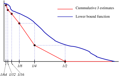
Figure 4: Lower bound function $\underline{f}^{(\boldsymbol{v})}(u)$ for $u\in(0,1]$ and cumulative J estimates on outcomes consistent with $\boldsymbol{v}$ $\int_{u}^{1}\hat{f}^{(J)}(x,\boldsymbol{v})dx$. The J estimate $\hat{f}^{(J)}(u,\boldsymbol{v})$ is the negated slope.

Lemma 6.1

The J estimator is well defined, is unbiased and nonnegative when (5) holds, and satisfies

$$\forall\rho\forall\boldsymbol{v},\ \int_{\rho}^{1}\hat{f}^{(J)}(u,\boldsymbol{v})du \leq\underline{f}(\rho,\boldsymbol{v})$$ (8)

$$\forall\rho\forall\boldsymbol{v},\int_{\rho}^{1}\hat{f}^{(J)}(u,\boldsymbol{v})du \geq\underline{f}(4\rho,\boldsymbol{v})\ .$$ (9)

Proof

We first argue that the constructions, which are presented relative to a particular choices of the data $\boldsymbol{v}$, produce a consistent estimator. For that, we have to show that for every outcome $S(\rho,\boldsymbol{v})$, the assigned value is the same for all vectors $\boldsymbol{z}\in V^{*}(\rho,\boldsymbol{v})$. Since $\underline{f}(\rho,\boldsymbol{v})=\underline{f}(\rho,\boldsymbol{z})$ for all $\boldsymbol{z}\in V^{*}(\rho,\boldsymbol{v})$, in particular this holds for $\rho=2^{-j}$, so the setting of the estimator for $u\in(2^{-j-1},2^{-j}]$ is the same for all $S(u,\boldsymbol{z})$ where $\boldsymbol{z}\in V^{*}(2^{-j},\boldsymbol{v})$ (also when $\boldsymbol{z}\not\in V^{*}(2^{-j-1},\boldsymbol{v})$). Therefore, the resulting estimator is consistently defined.

We show that the construction maintains the following invariant for $j\geq 1$:

$$\underline{f}(2^{-j+1},\boldsymbol{v})=\int_{2^{-j}}^{1}\hat{f}^{(J)}(u,\boldsymbol{v})du\ .$$ (10)

From the first step of the construction,

$$\int_{1/2}^{1}\hat{f}^{(J)}(u,\boldsymbol{v})du=\int_{1/2}^{1}2\underline{f}(1,\boldsymbol{v})du=\underline{f}(1,\boldsymbol{v})\ .$$

So (10) holds for $j=1$. Now we assume by induction that (10) holds for $j$ and establish that it holds for $j+1$. If $\underline{f}(2^{-j},\boldsymbol{v})=\underline{f}(2^{-j+1},\boldsymbol{v})$, then by the definition of the J estimator $\int_{2^{-j-1}}^{2^{-j}}\hat{f}^{(J)}(u,\boldsymbol{v})du=0$ and we get

$$\int_{2^{-j-1}}^{1}\hat{f}^{(J)}(u,\boldsymbol{v})du=\int_{2^{-j}}^{1}\hat{f}^{(J)}(u,\boldsymbol{v})du=\underline{f}(2^{-j+1},\boldsymbol{v})=\underline{f}(2^{-j},\boldsymbol{v})\ .$$

Otherwise, by definition, $\int_{2^{-j-1}}^{2^{-j}}\hat{f}^{(J)}(u,\boldsymbol{v})du=\underline{f}(2^{-j},\boldsymbol{v})-\underline{f}(2^{-j+1},\boldsymbol{v})$ and hence $\int_{2^{-j-1}}^{1}\hat{f}^{(J)}(u,\boldsymbol{v})du=\underline{f}(2^{-j},\boldsymbol{v})$ and (10) holds for $j+1$.

From monotonicity, $\underline{f}(2^{-j+1},\boldsymbol{v})\leq\underline{f}(2^{-j},\boldsymbol{v})$ and when substituting (10) in the definition of the estimator we obtain that the estimates are always nonnegative.

To establish (8) we use (10), the relation $2^{\lfloor\log_{2}\rho\rfloor}\leq\rho<2^{1+\lfloor\log_{2}\rho\rfloor}$, and monotonicity of $\underline{f}(u,\boldsymbol{v})$, to obtain

$$\int_{\rho}^{1}\hat{f}^{(J)}(u,\boldsymbol{v})du\leq\int_{2^{\lfloor\log_{2}\rho\rfloor}}^{1}\hat{f}^{(J)}(u,\boldsymbol{v})du=\underline{f}(2^{1+\lfloor\log_{2}\rho\rfloor},\boldsymbol{v})\leq\underline{f}(\rho,\boldsymbol{v})\ .$$

Similarly, we establish (9) using (10), and the relation $2^{-1+\lceil\log_{2}\rho\rceil}\leq\rho\leq 2^{\lceil\log_{2}\rho\rceil}$:

$$\int_{\rho}^{1}\hat{f}^{(J)}(u,\boldsymbol{v})du \geq\int_{2^{\lceil\log_{2}\rho\rceil}}^{1}\hat{f}^{(J)}(u,\boldsymbol{v})du=\underline{f}(2^{1+\lceil\log_{2}\rho\rceil},\boldsymbol{v})\geq\underline{f}(4\rho,\boldsymbol{v})$$

Lastly, unbiasedness follows from (5) and combining (8) and (9):

$$\underline{f}(\rho,\boldsymbol{v})\geq\int_{\rho}^{1}\hat{f}^{(J)}(u,\boldsymbol{v})du\geq\underline{f}(4\rho,\boldsymbol{v})\ .$$

when we take the limit as $\rho\rightarrow 0$.  
 

Computing the J estimate from an outcome $S$: From the outcome we know the seed value $\rho$ and the lower bound function $\underline{f}^{(\boldsymbol{v})}(u)$ for all $u\geq\rho$ (recall that the lower bound on this range is the same for all data $\boldsymbol{v}\in V^{*}(S)$, so we do not need to know the data $\boldsymbol{v}$). We compute $i\leftarrow\lfloor-\log_{2}\rho\rfloor$ and use the invariant (10) in the definition of J, obtaining the J estimate $2^{i+1}(\underline{f}(2^{-i},\boldsymbol{v})-\underline{f}(2^{-i+1},\boldsymbol{v}))$.

Example: We demonstrate the application of the J estimator through a simple example. The data domain in our example includes pairs $(v_{1},v_{2})$ of nonnegative reals. We are interested in $f(v_{1},v_{2})=(\max\{v_{1}-v_{2},0\})^{2}$, which sum aggregates to (the square of) the “one sided” Euclidean distance. The data is PPS sampled with threshold $\tau=1$ for both entries, therefore, the sampling probability of entry $i$ is $\min\{1,v_{i}\}$. Sampling is coordinated, which means that for a seed $\rho\in U[0,1]$, entry $i$ is sampled if and only if $v_{i}\geq\rho$. The outcome $S$ includes the values of the sampled entries and the seed value $\rho$. If no entry is sampled, or only the second entry is sampled, the lower bound function for $x\geq\rho$ is $0$ and the J estimate is $0$. If only the first entry is sampled, the lower bound function, for $x\geq\rho$, and accordingly, the J estimate are

$$\underline{f}^{(\boldsymbol{v})}(x) =\max\{0,v_{1}-x\}^{2}$$

$$\hat{f}^{(J)}(S) =2^{\lfloor-\log_{2}\rho\rfloor+1}\bigg{(}\max\{0,v_{1}-2^{-\lfloor-\log_{2}\rho\rfloor}\}^{2}-\max\{0,v_{1}-2^{1-\lfloor-\log_{2}\rho\rfloor}\}^{2}\bigg{)}\ .$$

If both entries are sampled, the lower bound function for $x\geq\rho$ and the $J$ estimate are

$$\underline{f}^{(\boldsymbol{v})}(x) =\max\{0,v_{1}-\max\{v_{2},x\}\}^{2}$$

$$\hat{f}^{(J)}(S) =2^{\lfloor-\log_{2}\rho\rfloor+1}\bigg{(}\max\{0,v_{1}-\max\{v_{2},2^{-\lfloor-\log_{2}\rho\rfloor}\}\}^{2}-\max\{0,v_{1}-\max\{v_{2},2^{1-\lfloor-\log_{2}\rho\rfloor}\}\}^{2}\bigg{)}\ .$$

6.1 Competitiveness of the J estimator

Theorem 6.1

The estimator $\hat{f}^{(J)}$ is $O(1)$-competitive.

Proof

We will show that

$$\forall\boldsymbol{v},\,\int_{0}^{1}\bigg{(}\hat{f}^{(J)}(u,\boldsymbol{v})\bigg{)}^{2}du\leq 84\int_{0}^{1}\bigg{(}\hat{f}^{(\boldsymbol{v})}(u)\bigg{)}^{2}du.$$

Let $\rho=2^{-j}$ for some integer $j\geq 0$. Recall the construction of $\hat{f}^{(J)}$ on an interval $(\rho/2,\rho]$. The value is fixed in the interval and is either $0$, if $\int_{\rho}^{1}\hat{f}^{(J)}(u,\boldsymbol{v})du=\underline{f}^{(\boldsymbol{v})}(\rho)$ or is $2\frac{\underline{f}^{(\boldsymbol{v})}(\rho)-\int_{\rho}^{1}\hat{f}^{(J)}(u,\boldsymbol{v})du}{\rho}$. Using (9) in Lemma 6.1, we obtain that for $u\in(\rho/2,\rho]$,

$$\hat{f}^{(J)}(u,\boldsymbol{v}) \leq 2\frac{\underline{f}^{(\boldsymbol{v})}(\rho)-\int_{\rho}^{1}\hat{f}^{(J)}(u,\boldsymbol{v})du}{\rho}\leq 2\frac{\underline{f}^{(\boldsymbol{v})}(\rho)-\underline{f}^{(\boldsymbol{v})}(4\rho)}{\rho}$$

Thus,

$$\int_{\rho/2}^{\rho}\bigg{(}\hat{f}^{(J)}(u,\boldsymbol{v})\bigg{)}^{2}du \leq\frac{\rho}{2}\frac{4}{\rho^{2}}\bigg{(}\underline{f}^{(\boldsymbol{v})}(\rho)-\underline{f}^{(\boldsymbol{v})}(4\rho)\bigg{)}^{2}=\frac{2}{\rho}\bigg{(}\underline{f}^{(\boldsymbol{v})}(\rho)-\underline{f}^{(\boldsymbol{v})}(4\rho)\bigg{)}^{2}$$ (11)

We now bound the expectation of $\hat{f}^{(\boldsymbol{v})}$ on $u\in(\rho/2,4\rho)$ from below.

$$\int_{\rho/2}^{4\rho}\hat{f}^{(\boldsymbol{v})}(u)du=\int_{\rho}^{4\rho}\hat{f}^{(\boldsymbol{v})}(u)du+\int_{\rho/2}^{\rho}\hat{f}^{(\boldsymbol{v})}(u)du$$

$$\geq \int_{\rho}^{4\rho}\hat{f}^{(\boldsymbol{v})}(u)du+\frac{\rho}{2}\hat{f}^{(\boldsymbol{v})}(\rho)$$ (12)

$$\geq \int_{\rho}^{4\rho}\hat{f}^{(\boldsymbol{v})}(u)du+\frac{\rho}{2}\frac{\underline{f}^{(\boldsymbol{v})}(\rho)-\int_{\rho}^{1}\hat{f}^{(\boldsymbol{v})}(u)du}{\rho}$$ (13)

$$= \int_{\rho}^{4\rho}\hat{f}^{(\boldsymbol{v})}(u)du++\frac{1}{2}\bigg{(}\underline{f}^{(\boldsymbol{v})}(\rho)-\int_{\rho}^{4\rho}\hat{f}^{(\boldsymbol{v})}(u)du-\int_{4\rho}^{1}\hat{f}^{(\boldsymbol{v})}(u)du\bigg{)}$$

$$= \frac{1}{2}\int_{\rho}^{4\rho}\hat{f}^{(\boldsymbol{v})}(u)du+\frac{1}{2}\bigg{(}\underline{f}^{(\boldsymbol{v})}(\rho)-\int_{4\rho}^{1}\hat{f}^{(\boldsymbol{v})}(u)du\bigg{)}\geq\frac{1}{2}\bigg{(}\underline{f}^{(\boldsymbol{v})}(\rho)-\underline{f}^{(\boldsymbol{v})}(4\rho)\bigg{)}$$ (14)

Inequality (12) follows from monotonicity of the function $\hat{f}^{(\boldsymbol{v})}$. Inequality (13) from the definition of $\hat{f}^{(\boldsymbol{v})}$ as the negated derivative of the lower hull of $\underline{f}^{(\boldsymbol{v})}$ $\hat{f}^{(\boldsymbol{v})}(\rho)\geq\frac{\underline{f}^{(\boldsymbol{v})}(\rho)-\int_{\rho}^{1}\hat{f}^{(\boldsymbol{v})}(u)du}{\rho}$ More precisely, we can use the explicit definition of the $\boldsymbol{v}$-optimal estimates (24) provided in Section A,

$$\hat{f}^{(\boldsymbol{v})}(\rho)=\inf_{0\leq\eta<\rho}\frac{\underline{f}^{(\boldsymbol{v})}(\eta)-\int_{\rho}^{1}\hat{f}(u,\boldsymbol{v})du}{\rho-\eta}\geq\inf_{0\leq\eta<\rho}\frac{\underline{f}^{(\boldsymbol{v})}(\rho)-\int_{\rho}^{1}\hat{f}(u,\boldsymbol{v})du}{\rho-\eta}=\frac{\underline{f}^{(\boldsymbol{v})}(\rho)-\int_{\rho}^{1}\hat{f}(u,\boldsymbol{v})du}{\rho}\ .$$

Lastly, inequality (14) uses $\int_{4\rho}^{1}\hat{f}^{(\boldsymbol{v})}(u)du\leq\underline{f}^{(\boldsymbol{v})}(4\rho)$, which follows from nonnegativity of $\hat{f}^{(\boldsymbol{v})}$ and Lemma 4.2.

Dividing both side by $3.5\rho$ we obtain a lower bound on the average value of $\hat{f}^{(\boldsymbol{v})}(u)$ in the interval $[\rho/2,4\rho]$.

$$\frac{1}{3.5\rho}\int_{\rho/2}^{4\rho}\hat{f}^{(\boldsymbol{v})}(u)du\geq\frac{1}{7\rho}\bigg{(}\underline{f}^{(\boldsymbol{v})}(\rho,\boldsymbol{v})-\underline{f}^{(\boldsymbol{v})}(4\rho)\bigg{)}$$ (15)

We next show that the value $\hat{f}^{(J)}(u,\boldsymbol{v})$ on $u\in(\rho/2,\rho]$ is at most some constant times the expected value of the square of $\hat{f}^{(\boldsymbol{v})}$ on $u\in(\rho/2,4\rho)$.

$$\int_{\rho/2}^{4\rho}\hat{f}^{(\boldsymbol{v})}(u)^{2}du\geq\int_{\rho/2}^{4\rho}\left(\frac{1}{3.5\rho}\int_{\rho/2}^{4\rho}\hat{f}^{(\boldsymbol{v})}(u)du\right)^{2}du\geq$$ (16)

$$\int_{\rho/2}^{4\rho}\left(\frac{1}{7\rho}\bigg{(}\underline{f}^{(\boldsymbol{v})}(\rho)-\underline{f}^{(\boldsymbol{v})}(4\rho)\bigg{)}\right)^{2}du\geq$$ (17)

$$3.5\rho\bigg{(}\frac{1}{7\rho}\bigg{)}^{2}\bigg{(}\underline{f}^{(\boldsymbol{v})}(\rho)-\underline{f}^{(\boldsymbol{v})}(4\rho)\bigg{)}^{2}\geq$$ (18)

$$\frac{1}{28}\int_{\rho/2}^{\rho}\hat{f}^{(J)}(u,\boldsymbol{v})^{2}du$$

Inequality (16) uses the fact that for any random variable $X$, $({\textsf{E}}[X])^{2}\leq{\textsf{E}}[X^{2}]$ applied to $\hat{f}^{(\boldsymbol{v})}$ for $u\in(\rho/2,4\rho]$. Inequality (17) follows from (15). Lastly, Inequality (18) follows from (11). We obtain

$$\int_{0}^{1}\hat{f}^{(J)}(u)^{2}du =\sum_{i=0}^{\infty}\int_{2^{-i-1}}^{2^{-i}}\hat{f}^{(J)}(u)^{2}du$$

$$\leq 28\sum_{i=0}^{\infty}\int_{2^{-i-1}}^{\min\{1,2^{-i+2}\}}\hat{f}^{(\boldsymbol{v})}(u)^{2}du\leq 28\cdot 3\int_{0}^{1}\hat{f}^{(\boldsymbol{v})}(u)^{2}du$$

 
 

7 Proof of Theorem 5.1

Proof

$\bullet$ “$\Rightarrow$” (5): From Lemma 4.2, an unbiased and nonnegative estimator $\hat{f}$ must satisfy (3). Fixing $\boldsymbol{v}$ in (3) and taking the limit as $\rho\rightarrow 0$ we obtain that ${\textsf{E}}[\hat{f}|\boldsymbol{v}]=\int_{0}^{1}\hat{f}(u,\boldsymbol{v})du\leq\lim_{u\rightarrow 0}\underline{f}^{(\boldsymbol{v})}(u,\boldsymbol{v})$. Combining with unbiasedness: ${\textsf{E}}[\hat{f}|\boldsymbol{v}]=f(\boldsymbol{v})$ we obtain (5).

$\bullet$ “$\Leftarrow$” (5): Follows immediately from Lemma 6.1.

$\bullet$ “$\Rightarrow$” (7): We bound from below the contribution to the expectation of unbiased and nonnegative $\hat{f}$ of outcomes $S(u,\boldsymbol{v})$ for $u\leq\rho$: $\int_{0}^{\rho}\hat{f}(u,\boldsymbol{v})=\int_{0}^{1}\hat{f}(u,\boldsymbol{v})-\int_{\rho}^{1}\hat{f}(u,\boldsymbol{v})\geq f(\boldsymbol{v})-\underline{f}^{(\boldsymbol{v})}(u)$. The last inequality follows from unbiasedness and nonnegativity (3). Hence, the average value $\hat{f}(u,\boldsymbol{v})$ when $u<\rho$ must be at least $\frac{f(\boldsymbol{v})-\underline{f}^{(\boldsymbol{v})}(\rho)}{\rho}$, and thus, considering all possible values of $\rho>0$, we obtain that $\hat{f}$ can be bounded only if it satisfies (7).

$\bullet$ “$\Leftarrow$” (7): Note that (7) $\implies$ (5), and therefore the conditions of Lemma 6.1 are satisfied and the J estimator is well defined, nonnegative, and unbiased. It remains to show that given (7), or the equivalent statement

$$\forall\boldsymbol{v}\,\exists c<\infty\,\forall u,\,f(v)-\underline{f}^{(\boldsymbol{v})}(u)\leq cu\ ,$$ (19)

the J estimator is bounded. Fix $\boldsymbol{v}$ and let $c$ be as in (19).

$$\hat{f}^{(J)}(\rho,\boldsymbol{v}) \leq 2\frac{\underline{f}^{(\boldsymbol{v})}(\rho/2)-\int_{2\rho}^{1}\hat{f}^{(J)}(u,\boldsymbol{v})du}{\rho}$$ (20)

$$\leq 2\frac{f(\boldsymbol{v})-\underline{f}^{(\boldsymbol{v})}(8\rho)}{\rho}$$ (21)

$$=16\frac{f(\boldsymbol{v})-\underline{f}^{(\boldsymbol{v})}(8\rho)}{8\rho}\leq 16c$$ (22)

Inequality (20) is from the definition of the J estimator. Inequality (21) uses definition of the lower bound function and (9). Lastly, (22) follows from our assumption (19).

$\bullet$ “$\iff$” (6): From Theorem 4.1, for all $\boldsymbol{v}$, (6), which is square-integrability of $\hat{f}^{(\boldsymbol{v})}(u)$, is necessary for existence of a nonnegative unbiased estimator with finite variance for $\boldsymbol{v}$. Sufficiency follows from the proof of Theorem 6.1, which shows that for all $\boldsymbol{v}$, the expectation of the square of the J estimator is at most a constant times the minimum possible, and (2), which states that the variance is bounded if and only if the expectation of the square is bounded.  
 

Conclusion

We developed a precise understanding of the queries we can estimate accurately over coordinated shared-seed samples. We defined variance competitiveness, and showed that $O(1)$ competitiveness is always attainable when estimators with finite variances exist. Our work uses a fresh, CS-inspired, and unified approach to the study of estimators that is particularly suitable for data analysis from samples and sets the ground for continued work.

In a follow up work [15], aiming for good performance in practice, we seek estimators that are variance optimal (admissible [32]), that is, can not be strictly improved. We show that there is a range of variance optimal and competitive estimators and that this choice can be leveraged to obtain natural estimators with desired properties or customized estimators to patterns in our data: The L^∗ estimator, which is defined for any function for which a nonnegative unbiased estimator exists, is the unique monotone variance-optimal estimator and is guaranteed to have a ratio of at most $4$. Customization is facilitated by deriving order-optimal estimators which optimize variances with respect to (any) specified priorities over the data domain. The L^∗ estimator prioritizes data on which the estimated function is smaller whereas the U^∗ estimator prioritizes large values. We demonstrate the potential for applications in [16], for $L_{p}$ difference estimation and in [9], for sketch-based similarity estimation in massive graphs.

A natural question is to bound the best possible competitive ratio. That is, the supremum over instances (data domain, shared-seed sampling scheme, and function) for which unbiased nonnegative estimators with finite variances exist of the best ratio attainable for the instance. The L^∗ estimator in [15] gives an upper bound of $4$ and we were able to provide a tighter upper bound of $3.375$ and a lower bound of $1.44$. An interesting question is to close this gap.

In the future, we hope to build on our understanding of coordinated sampling to extend our treatment of independent sampling in [14]. We envision automated tools that provide estimates according to specifications of the sampling scheme, query, competitive ratio, and prioritization of patterns in the data.

Appendix A Pointwise variance optimality

We work with partial specification of (nonnegative unbiased) estimators. A partial specification $\hat{f}$ is defined over a subset ${\cal S}$ of outcomes that is closed under the containment order $V^{*}(S)$:

$$\forall\boldsymbol{v}\ \exists\rho_{v}\in[0,1],\ S(u,\boldsymbol{v})\in{\cal S}\,\mbox{{\it a.e.} for }u>\rho_{v}\,\wedge\,$$

$$S(u,\boldsymbol{v})\not\in{\cal S}\,\mbox{{\it a.e.} for }u\leq\rho_{v}\ .$$

We also require that $\hat{f}:{\cal S}\geq 0$, that is, estimates are nonnegative when specified, and that

$$\forall\boldsymbol{v},\ \rho_{v}>0 \implies \int_{\rho_{v}}^{1}\hat{f}(u,\boldsymbol{v})du\leq f(\boldsymbol{v})$$ (23a)

$$\forall\boldsymbol{v},\ \rho_{v}=0 \implies \int_{\rho_{v}}^{1}\hat{f}(u,\boldsymbol{v})du=f(\boldsymbol{v})$$ (23b)

If $\rho_{v}=0$, we say that the estimator is fully specified for $\boldsymbol{v}$.

We show that a partial specification $\hat{f}$ can always be extended to an unbiased nonnegative estimator:

Lemma A.1

If $f$ satisfies (5) (has a nonnegative unbiased estimator) and $\hat{f}$ is partially specified then it can be extended to an unbiased nonnegative estimator.

Proof

The only if direction follows from Lemma 4.2. The “if” direction follows from a slight modification of the J estimator construction, in which we “start” to specify the estimator at $\rho_{v}$ instead of $1$.  
 

Theorem A.1

If $\hat{f}$ is a partially specified estimator, then an extension of $\hat{f}$ to the outcomes $S(\rho,\boldsymbol{v})$ for $\rho\in(0,\rho_{v}]$ is a partially specified estimator and minimizes $\mbox{\sc var}[\hat{f}|\boldsymbol{v}]$ (over all unbiased and nonnegative estimators which are extensions of the partial specification $\hat{f}$).

$$\iff\ \text{for $u\in(0,\rho_{v}]$ {\it a.e.}}$$

$$\hat{f}(u,\boldsymbol{v}) = \inf_{0\leq\eta<u}\frac{\underline{f}^{(\boldsymbol{v})}(\eta)-\int_{u}^{1}\hat{f}(x,\boldsymbol{v})dx}{u-\eta}\ .$$ (24)

Moreover, a solution $\hat{f}$ of (24) always exists and $H(u)=\int_{u}^{1}\hat{f}(x,\boldsymbol{v})dx$ for $u\in(0,\rho_{v}]$ is unique.

Proof

From Lemma A.1 an extended $\hat{f}$ to outcomes $S(\eta,\boldsymbol{v})$ for $\eta\in(0,\rho_{v}]$ is a partially specified estimator if and only if

$$\forall u\leq\rho_{v}\ \int_{u}^{1}\hat{f}(x,\boldsymbol{v})dx\leq\underline{f}^{(\boldsymbol{v})}(u)\$$ (25a)

$$\int_{0}^{1}\hat{f}(x,\boldsymbol{v})dx=f(\boldsymbol{v})$$ (25b)

From the structure of the constraints (25), if we take a solution $$\hat{f}(u,\boldsymbol{v}) u \hat{f} u u (0,\rho_{v}]$$ and shift “weight” to lower values (decreasing on higher values and increasing on lower ones so that the total contribution is the same) then the result is also a solution. If the shift results in decrease of higher values and increase of lower values, then the variance decreases. Therefore, a minimum variance solution of (25) must be monotone nonincreasing with almost everywhere, meaning, that monotonicity holds if we exclude from a set of points with zero measure.

$$\exists\text{zero measure $U^{0}\subset(0,\rho_{v}]$}\forall u_{1},u_{2}\in(0,\rho_{v}]\setminus U_{0},$$

$$u_{1}<u_{2}\implies\hat{f}(u_{1},\boldsymbol{v})\geq\hat{f}(u_{2},\boldsymbol{v})$$ (25c)

Looking now only at extensions satisfying (25a), (25b), and (25c), we can decrease variance if we could ”shift weight” from the higher estimates on lower $u$ values to the lower estimates on higher $u$ values. Such shifts, however, may violate (25a). Therefore, an estimator has minimum variance only if all such shifts result in violation, that is, after excluding a zero measure set, between any two points with strictly different estimate values there must be a point $\eta$ such that $\int_{\eta}^{1}\hat{f}(u,\boldsymbol{v})du$ “touches” the lower bound at $\eta$. Formally,

$$\exists\text{ zero measure $U^{0}\subset(0,\rho_{v}]$}\forall u_{1},u_{2}\in(0,\rho_{v}]\setminus U_{0}$$

$$u_{1}<u_{2}\wedge\hat{f}(u_{1},\boldsymbol{v})>\hat{f}(u_{2},\boldsymbol{v}) \implies$$

$$\exists\eta\in(u_{1},u_{2}],\int_{\eta}^{1}\hat{f}(u,\boldsymbol{v})du=\lim_{u\rightarrow\eta^{+}}\underline{f}^{(\boldsymbol{v})}(u)\ .$$ (25d)

We established that (25) ((25a)- (25d)) are necessary for an extension to have minimum variance. We also argued that any extension satisfying (25a) and (25b) can be transformed to one satisfying (25c) and (25d) without increasing its variance. Therefore, if we can establish that (25) have a unique solution (up to equivalence), the solution must have minimum variance.

Geometrically, an extension $\hat{f}$ satisfies either (25) or (24) if and only if the function $H(u)=\int_{u}^{1}\hat{f}(x,\boldsymbol{v})dx$ is the lower boundary of the convex hull of the lower bound function $\underline{f}^{(\boldsymbol{v})}(x)$ for $x\in(0,\rho_{v}]$ and the point $(\rho_{v},\int_{\rho_{v}}^{1}\hat{f}(u,\boldsymbol{v})du)$. This implies existence and uniqueness of the solution and also that it has the desired properties.

We provide an algebraic proof. We start by exploring the structure which an extension of $\hat{f}(u,\boldsymbol{v})$ to $u\in(0,\rho_{v}]$, which satisfies (24), must have. We subsequently use the structure to establish existence and nonnegativity, uniqueness (a.e.), that it satisfies (25), and lastly, to show that any function that violates (24) must also violate (25). The combination of these properties implies the claim of the theorem.

Structure: We say that $\rho$ is an LB (lower bound) point of $\hat{f}(u,\boldsymbol{v})$ if the infimum of the solution of (24) at $\rho$ is achieved as $\eta\rightarrow\rho^{-}$, that is,

$$\hat{f}(\rho,\boldsymbol{v})=\lim_{\eta\rightarrow\rho^{-}}\frac{\underline{f}^{(\boldsymbol{v})}(\eta)-\int_{\rho}^{1}\hat{f}(u,\boldsymbol{v})du}{\rho-\eta}\ .$$

Otherwise, if the infimum is approached when $\eta<\rho-\epsilon$ for some $\epsilon>0$, we say that $\rho$ is a gap point. Note that it is possible for $\rho$ to be both an LB and a gap point if the infimum is approached at multiple places. If

$$\int_{\rho}^{1}\hat{f}(u,\boldsymbol{v})du<\lim_{\eta\rightarrow\rho^{-}}\underline{f}^{(\boldsymbol{v})}(\eta)=\underline{f}^{(\boldsymbol{v})}(\rho)\ ,$$

then $\rho$ must be a gap point, and if equality holds, $\rho$ can be either an LB or a gap point (or both). The equality follows using Corollary 4.1 (left continuity of $\underline{f}^{(\boldsymbol{v})}$).

We use this classification of points to partition $(0,\rho_{v}]$ into LB and gap subintervals of the form $(y,\rho]$, that is, open to the left and closed to the right.

LB subintervals are maximal subintervals containing exclusively LB points (which can double as gap points) that have the form $(y,\rho]$. From left continuity and monotonicity of $\underline{f}^{(\boldsymbol{v})}$, if $\rho$ is an LB point and not a gap point then there is some $\epsilon>0$ such that $(x-\epsilon,x]$ are also LB points. Thus all LB points that are not gap points must be part of LB subintervals and these subintervals are open to the left and closed to the right (the point $y$ is a gap point which may double as an LB point). Alternatively, we can identify LB subintervals as maximal such that

$$\forall x\in(y,\rho],\ \int_{x}^{1}\hat{f}(u,\boldsymbol{v})du=\underline{f}^{(\boldsymbol{v})}(x)\ .$$

Gap subintervals are maximal that satisfy

$$\forall x\in(y,\rho),\ \int_{x}^{1}\hat{f}(u,\boldsymbol{v})du<\lim_{u\rightarrow x^{+}}\underline{f}^{(\boldsymbol{v})}(u)\ .$$ (26)

Note that a consecutive interval of gap points may consist of multiple back-to-back gap subintervals.

We can verify that the boundary points $b\in\{y,\rho\}$ of both LB and gap subintervals satisfy

$$\int_{b}^{1}\hat{f}(u,\boldsymbol{v})du=\lim_{x\rightarrow b^{+}}\underline{f}^{(\boldsymbol{v})}(x)$$ (27)

Visually, LB intervals are segments where $\int_{u}^{1}\hat{f}(x,\boldsymbol{v})dx$ “identifies” with the lower bound function whereas gap intervals are linear segments where it “skips” between two points where it touches (in the sense of limit from the right) the (left-continuous) lower bound function. Figure 3 illustrates a partition of an example lower bound function and its lower hull into gap and LB subintervals. From left to right, there are two gap subintervals, an LB subinterval, a gap subinterval, and finally a trivial LB subinterval (where the LB and estimates are $0$).

Existence, nonnegativity, and (25a) :

For some $0<\rho\leq\rho_{v}$, let $\hat{f}(u,\boldsymbol{v})$ be an extension which satisfies (24) and (25a) for all $u\in(\rho,\rho_{v}]$. We show that there exists $y<\rho$ such that the solution can be extended to $(y,\rho]$, that is, (24) and (25a) are satisfied also for $u\in(y,\rho]$.

Consider the solution of (24) at $u=\rho$. If the infimum is attained at $\eta<\rho$, let $y$ be the infimum over points $\eta$ that attain the infimum of (24) at $\rho$. We can extend the solution of (24) to the interval $(y,\rho]$, which is a gap interval (or the prefix of one). The solution is fixed throughout the interval:

$$\forall x\in(y,\rho],\ \hat{f}(x,\boldsymbol{v})=\frac{\displaystyle{\lim_{\eta\rightarrow y^{+}}}\underline{f}^{(\boldsymbol{v})}(\eta)-\displaystyle{\lim_{\eta\rightarrow\rho^{+}}}\underline{f}^{(\boldsymbol{v})}(\eta)}{\rho-y}\ .$$ (28)

Assume now that the infimum of the solution of (24) at $\rho$ is attained as $\eta\rightarrow\rho^{-}$ and not at any $\eta<\rho$. Let $y$ be the supremum of points $x<\rho$

$$\inf_{0\leq\eta<x}\frac{\underline{f}^{(\boldsymbol{v})}(\eta)-\lim_{u\rightarrow x^{+}}\underline{f}^{(\boldsymbol{v})}(u)}{x-\eta}<\lim_{\eta\rightarrow x^{-}}\frac{\underline{f}^{(\boldsymbol{v})}(\eta)-\lim_{u\rightarrow x^{+}}\underline{f}^{(\boldsymbol{v})}(u)}{x-\eta}$$ (29)

(We allow the rhs to be $+\infty$). We have $y<\rho$ and can extend the solution to $(y,\rho]$. The extension satisfies $\int_{x}^{1}\hat{f}(u,\boldsymbol{v})du=\underline{f}^{(\boldsymbol{v})}(x)$ and $(y,\rho]$ is an LB subinterval or a prefix of one. The actual estimator values on $(y,\rho]$ are the negated left derivative of $\underline{f}^{(\boldsymbol{v})}(u)$:

$$\forall x\in(y,\rho],\hat{f}(x,\boldsymbol{v})=\lim_{\eta\rightarrow x^{-}}\frac{\underline{f}^{(\boldsymbol{v})}(\eta)-\underline{f}^{(\boldsymbol{v})}(x)}{x-\eta}$$

In both cases (where the extension corresponds to an LB or gap subinterval), the solution on $(y,\rho]$ exists, is nonnegative, and satisfies (25a) for $u\in(y,\rho]$.

Thus, starting from $u=\rho_{v}$, we can iterate the process and compute a solution on a suffix of $(0,\rho_{v}]$ that is partitioned into gap and LB intervals. The sum of sizes of intervals, however, may converge to a value $<\rho_{v}$ and thus the process may not converge to covering $(0,\rho_{v}]$. To establish existence, assume to the contrary that there is no solution that covers $(0,\rho_{v}]$. Let $x$ be the infimum such that there are solutions on $(x,\rho_{v}]$ but there are no solutions for $(x-\epsilon,\rho_{v}]$ for all $\epsilon>0$. Let $\hat{f}(u,\boldsymbol{v})$ be a solution on $u\in(x,\rho_{v}]$ and consider its partition to LB and gap intervals. Each interval that intersects $[x,x+\epsilon)$ must contain a left boundary point $y_{\epsilon}$ of some subinterval (it is possible that $y_{\epsilon}=x$). All boundary points satisfy $\int_{y_{\epsilon}}^{1}\hat{f}(x,\boldsymbol{v})\leq\underline{f}^{(\boldsymbol{v})}(y_{\epsilon})$. We have

$$\int_{x}^{1}\hat{f}(u,\boldsymbol{v})du = \lim_{\epsilon\rightarrow 0}\int_{y_{\epsilon}}^{1}\hat{f}(x,\boldsymbol{v})\leq\lim_{\epsilon\rightarrow 0}\underline{f}^{(\boldsymbol{v})}(y_{\epsilon})$$

$$= \lim_{\eta\rightarrow x^{+}}\underline{f}^{(\boldsymbol{v})}(\eta)\leq\underline{f}^{(\boldsymbol{v})}(x)$$

The last inequality follows from monotonicity of $\underline{f}^{(\boldsymbol{v})}(u)$. Thus, we can apply our extension process starting from $\rho=x$ and extend the solution to $(y,x]$ for some $y<x$, contradicting our assumption and establishing existence.

Uniqueness: Assume there are two different solutions and let $x\in(0,\rho_{v})$ be the supremum of values on which they differ. Consider one of the solutions. $x$ can not be an interior point of a (gap or LB) subinterval because the estimator is determined on the subinterval from values on the right boundary, which is the same for both solutions. If $x$ is a right boundary point, $\int_{x}^{\rho_{v}}\hat{f}(u,\boldsymbol{v})du$ is same for both functions and thus the left boundary and the solution on the interval are uniquely determined and must be the same for both functions, contradicting our assumption.

Satisifes (25b) (unbiasedness): From (5) (a sufficient necessary condition to existence of unbiased nonnegative estimator) and (27)

$$\int_{0}^{1}\hat{f}(u,\boldsymbol{v})du=\lim_{u\rightarrow 0^{+}}\underline{f}^{(\boldsymbol{v})}(u)=f(\boldsymbol{v}).$$

Satisifes (25c) and (25d): Within an LB subinterval the estimator must be nonincreasing, since otherwise we obtain a contradiction to the definition of an LB point. The fixed values on two consecutive gap intervals $(y,x]$ and $(x,\rho]$ must also be nonincreasing because otherwise the infimum of the solution at $\rho$ could not be obtained at $x$ since a strictly lower value is obtained at $y$.

The only solution of (25): Let $\hat{f}^{(\boldsymbol{v})}(u)\equiv\hat{f}(u,\boldsymbol{v})$ where $\hat{f}$ is a solution of (24). Let $\hat{f}^{\prime}$ be another extension which satisfies (25a) and (25b) (and thus constitutes a partially specified estimator that is fully specified on $\boldsymbol{v}$) but is not equivalent to $\hat{f}^{(\boldsymbol{v})}$, that is, for some $\rho$

$$\int_{\rho}^{\rho_{v}}\hat{f}^{(\boldsymbol{v})}(u)du\not=\int_{\rho}^{\rho_{v}}\hat{f}^{\prime}(u,\boldsymbol{v})du\ .$$

We show that $\hat{f}^{\prime}$ must violate (25c) or (25d).

We first show that if

$$\int_{\rho}^{\rho_{v}}\hat{f}^{(\boldsymbol{v})}(u)du<\int_{\rho}^{\rho_{v}}\hat{f}^{\prime}(u,\boldsymbol{v})du$$ (30)

then monotonicity (25c) must be violated. Let $\overline{\rho}$ be the supremum of points satisfying (30). Then $\overline{\rho}$ must be a gap point and some neighborhood to its left must be gap points. Let $y<\overline{\rho}$ be the left boundary point of this gap interval. Recall that $\hat{f}^{(\boldsymbol{v})}$ is constant on a gap interval.

Let $\rho\in(y,\overline{\rho})$ be such that (30) holds. There must be measurable set in $[\rho,\overline{\rho}]$ on which $\hat{f}^{\prime}>\hat{f}^{(\boldsymbol{v})}$. Since $y$ is a left boundary of a gap interval, from (27),

$$\int_{y}^{1}\hat{f}^{(\boldsymbol{v})}(u)du=\lim_{u\rightarrow y^{+}}\underline{f}^{(\boldsymbol{v})}(u)$$

and therefore, since $\hat{f}^{\prime}$ satisfies (25a), $\int_{y}^{\rho_{v}}\hat{f}^{\prime}du\leq\int_{y}^{\rho_{v}}\hat{f}^{(\boldsymbol{v})}(u)du$. Thus, there must exist a measurable subset of $[y,\rho]$ on which $\hat{f}^{\prime}<\hat{f}^{(\boldsymbol{v})}$. Since $\hat{f}^{(\boldsymbol{v})}$ is constant in $(y,\overline{\rho}]$, $\hat{f}^{\prime}$ violates (25c).

Lastly, we show that if

$$\int_{\rho}^{\rho_{v}}\hat{f}^{(\boldsymbol{v})}(u)du>\int_{\rho}^{\rho_{v}}\hat{f}^{\prime}(u,\boldsymbol{v})du$$ (31)

then even if (25c) holds then (25d) is violated.

There must exist a measurable subset $U\subset[\rho,\rho_{v}]$ on which $\hat{f}^{(\boldsymbol{v})}(u)>\hat{f}^{\prime}(u,\boldsymbol{v})$.

Let $\eta$ be the supremum of points $x\in[0,\rho)$ satisfying $\int_{x}^{\rho_{v}}\hat{f}^{\prime}(u,\boldsymbol{v})du=\lim_{u\rightarrow x^{+}}\underline{f}^{(\boldsymbol{v})}(u)$. Since this is satisfied by $x=0$ and the supremum can not be satisfied by $\rho$, such $\eta<\rho$ is well defined.

Since $\hat{f}^{(\boldsymbol{v})}$ satisfies (25a), $\int_{\eta}^{\rho_{v}}\hat{f}^{(\boldsymbol{v})}(u)du\leq\int_{\eta}^{\rho_{v}}\hat{f}^{\prime}(u,\boldsymbol{v})du$. Therefore, there must be another measurable set $W\subset[\eta,\rho]$ on which $\hat{f}^{(\boldsymbol{v})}(u)<\hat{f}^{\prime}(u,\boldsymbol{v})$. Because $\hat{f}^{(\boldsymbol{v})}$ is monotone, the values of $\hat{f}^{\prime}$ on $W$ are strictly larger than on $U$. Hence, $\hat{f}^{\prime}$ violates (25d).  

Theorem 4.1 follows by applying Theorem A.1 to an empty specification.

Appendix B Using sum estimators with bottom-$k$ sampling

We provide details on the application of sum estimators with bottom-$k$ sampling of instances. A technical requirement for applying sum estimators is that the sampling scheme of each item is explicit. This naturally happens with Poisson sampling where an entry (item $h$ in instance $i$) is sampled $\iff$ $r(u(h),v(h))\geq T_{i}(h)$. With bottom-$k$ sampling, however, item inclusions are dependent and therefore the separation a bit more technical, and relies on a technique named rank conditioning [12, 1].

Rank conditioning was applied to estimate subset sums over bottom-$k$ samples of a single instance, and allows us to treat each entry as Poisson sampled. In rough details, for each entry, we obtain a “$T_{i}(h)$ substitute” which allows the inclusion of $h$ in the sample of instance $i$ on seeds (and thus ranks) of all other items being fixed. With this conditioning, the inclusion of $h$ in the sample of $i$ is Poisson with threshold $T_{i}$, that is, follows the rule $r(u(h),v(h))\geq T_{i}$, where $T_{i}$ is equal to the $k$th largest rank value of items in instance $i$ with $h$ excluded which is the same as the $(k+1)$st largest rank value.

References

- [1] N. Alon, N. Duffield, M. Thorup, and C. Lund. Estimating arbitrary subset sums with few probes. In Proceedings of the 24th ACM Symposium on Principles of Database Systems, pages 317–325, 2005.
- [2] K. S. Beyer, P. J. Haas, B. Reinwald, Y. Sismanis, and R. Gemulla. On synopses for distinct-value estimation under multiset operations. In SIGMOD, pages 199–210. ACM, 2007.
- [3] K. R. W. Brewer, L. J. Early, and S. F. Joyce. Selecting several samples from a single population. Australian Journal of Statistics, 14(3):231–239, 1972.
- [4] A. Z. Broder. On the resemblance and containment of documents. In Proceedings of the Compression and Complexity of Sequences, pages 21–29. IEEE, 1997.
- [5] A. Z. Broder. Identifying and filtering near-duplicate documents. In Proceedings of the 11th Annual Symposium on Combinatorial Pattern Matching, volume 1848 of LNCS, pages 1–10. Springer, 2000.
- [6] J. W. Byers, J. Considine, M. Mitzenmacher, and S. Rost. Informed content delivery across adaptive overlay networks. IEEE/ACM Trans. Netw., 12(5):767–780, October 2004.
- [7] E. Cohen. Size-estimation framework with applications to transitive closure and reachability. J. Comput. System Sci., 55:441–453, 1997.
- [8] E. Cohen. All-distances sketches, revisited: Scalable estimation of the distance distribution and centralities in massive graphs. Technical Report cs.DS/1306.3284, arXiv, 2013.
-
[9]
E. Cohen, D. Delling, F. Fuchs, A. Goldberg, M. Goldszmidt, and R. Werneck.
Scalable similarity estimation in social networks:
closeness, node labels, and random edge lengths. In COSN, 2013. - [10] E. Cohen and H. Kaplan. Spatially-decaying aggregation over a network: model and algorithms. J. Comput. System Sci., 73:265–288, 2007.
- [11] E. Cohen and H. Kaplan. Summarizing data using bottom-k sketches. In Proceedings of the ACM PODC’07 Conference, 2007.
- [12] E. Cohen and H. Kaplan. Tighter estimation using bottom-k sketches. In Proceedings of the 34th VLDB Conference, 2008.
- [13] E. Cohen and H. Kaplan. Leveraging discarded samples for tighter estimation of multiple-set aggregates. In Proceedings of the ACM SIGMETRICS’09 Conference, 2009.
- [14] E. Cohen and H. Kaplan. Get the most out of your sample: Optimal unbiased estimators using partial information. In Proc. of the 2011 ACM Symp. on Principles of Database Systems (PODS 2011). ACM, 2011. full version: http://arxiv.org/abs/1203.4903.
- [15] E. Cohen and H. Kaplan. A case for customizing estimators: Coordinated samples. Technical Report cs.ST/1212.0243, arXiv, 2012.
- [16] E. Cohen and H. Kaplan. How to estimate change from samples. Technical Report cs.DS/1203.4903, arXiv, 2012.
- [17] E. Cohen, H. Kaplan, and S. Sen. Coordinated weighted sampling for estimating aggregates over multiple weight assignments. Proceedings of the VLDB Endowment, 2(1–2), 2009. full version: http://arxiv.org/abs/0906.4560.
- [18] E. Cohen, Y.-M. Wang, and G. Suri. When piecewise determinism is almost true. In Proc. Pacific Rim International Symposium on Fault-Tolerant Systems, pages 66–71, December 1995.
- [19] A. Das, M. Datar, A. Garg, and S. Rajaram. Google news personalization: scalable online collaborative filtering. In WWW, 2007.
- [20] N. Duffield, M. Thorup, and C. Lund. Priority sampling for estimating arbitrary subset sums. J. Assoc. Comput. Mach., 54(6), 2007.
- [21] P. S. Efraimidis and P. G. Spirakis. Weighted random sampling with a reservoir. Inf. Process. Lett., 97(5):181–185, 2006.
- [22] P. Gibbons and S. Tirthapura. Estimating simple functions on the union of data streams. In Proceedings of the 13th Annual ACM Symposium on Parallel Algorithms and Architectures. ACM, 2001.
- [23] P. B. Gibbons. Distinct sampling for highly-accurate answers to distinct values queries and event reports. In International Conference on Very Large Databases (VLDB), pages 541–550, 2001.
- [24] A. Gionis, P. Indyk, and R. Motwani. Similarity search in high dimensions via hashing. In Proceedings of the 25th International Conference on Very Large Data Bases, VLDB ’99, 1999.
- [25] M. Hadjieleftheriou, X. Yu, N. Koudas, and D. Srivastava. Hashed samples: Selectivity estimators for set similarity selection queries. In Proceedings of the 34th VLDB Conference, 2008.
- [26] J. Hájek. Sampling from a finite population. Marcel Dekker, New York, 1981.
- [27] D. G. Horvitz and D. J. Thompson. A generalization of sampling without replacement from a finite universe. Journal of the American Statistical Association, 47(260):663–685, 1952.
- [28] P. Indyk. Stable distributions, pseudorandom generators, embeddings and data stream computation. In Proc. 41st IEEE Annual Symposium on Foundations of Computer Science, pages 189–197. IEEE, 2001.
- [29] P. Indyk and R. Motwani. Approximate nearest neighbors: Towards removing the curse of dimensionality. In Proc. 30th Annual ACM Symposium on Theory of Computing, pages 604–613. ACM, 1998.
- [30] J. Lanke. On UMV-estimators in survey sampling. Metrika, 20(1):196–202, 1973.
- [31] D. Mosk-Aoyama and D. Shah. Computing separable functions via gossip. In Proceedings of the ACM PODC’06 Conference, 2006.
- [32] P. Mukhopandhyay. Theory and Methods of Survey Sampling. PHI learning, New Delhi, 2 edition, 2008.
- [33] E. Ohlsson. Sequential poisson sampling. J. Official Statistics, 14(2):149–162, 1998.
- [34] E. Ohlsson. Coordination of pps samples over time. In The 2nd International Conference on Establishment Surveys, pages 255–264. American Statistical Association, 2000.
- [35] B. Rosén. Asymptotic theory for successive sampling with varying probabilities without replacement, I. The Annals of Mathematical Statistics, 43(2):373–397, 1972.
- [36] B. Rosén. Asymptotic theory for order sampling. J. Statistical Planning and Inference, 62(2):135–158, 1997.
- [37] P. J. Saavedra. Fixed sample size pps approximations with a permanent random number. In Proc. of the Section on Survey Research Methods, Alexandria VA, pages 697–700. American Statistical Association, 1995.
- [38] M. Szegedy. The DLT priority sampling is essentially optimal. In Proc. 38th Annual ACM Symposium on Theory of Computing. ACM, 2006.