Kinematic Cusps With Two Missing Particles I:
Antler Decay Topology

Abstract

The kinematics of a final state system with two invisible particles and two visible particles can develop cusped peak structures. This happens when the system has a fixed invariant mass (such as from a narrow resonant particle decay or with a fixed collision c.m. energy) and undergoes decays of two on-shell intermediate particles. Focusing on the “antler decay topology”, we derive general analytic expressions for the invariant mass distribution and the kinematic cusp position. The sharp cusp peaks and the endpoint positions can help to determine the masses of the missing particles and the intermediate particles. We also consider transverse momentum variables and angular variables. In various distributions the kinematic cusp peaks are present and pronounced. We also study the effects on such kinematic cusp structures from realistic considerations including finite decay widths, the longitudinal boost of the system, and spin correlations.

I Introduction

With the advent of the Large Hadron Collider (LHC), the TeV scale physics will be fully explored in the coming decades. Most pressing of all to learn is the mechanism of the electroweak symmetry breaking and the related underlying dynamics beyond the standard model (SM). Among many interesting phenomena associated with the new physics at the TeV scale, the signature of events with large missing energy is one of the most exciting possibilities at the LHC. This is expected from new particles that do not leave any trace in the hadronic and electromagnetic components of the detector. These new missing particles may help to address one of the most profound puzzles in cosmology: what constitutes nearly a quarter of the energy density of our current universe in a form of cold dark matter (CDM) WMAP . The thermal history of the early universe suggests that a stable neutral particle of the electroweak-scale mass and interaction, called the Weakly Interacting Massive Particles (WIMP), is a plausible explanation of CDM WIMP and may be discovered as a missing particle at TeV-scale colliders.

Missing energy signal is generic in many new physics models. Additional discrete symmetry is often introduced to prohibit dangerous processes such as proton decay and to make the model compatible with the electroweak precision tests. Such a discrete symmetry (or parity) often needs nontrivial representations of new particles, while it assigns vanishing charges (or trivial representation) to the SM particles. Therefore, the lightest new particle is stable, becoming a natural candidate for the CDM particle. One of the most studied examples is the lightest neutralino in supersymmetric (SUSY) theories with $R$-parity conservation SUSY:DM . Other examples include the lightest Kaluza-Klein (KK) particle in universal extra dimensional (UED) theories with KK parity conservation DMExtraD , and the heavy photon in the little Higgs models with $T$-parity conservation (LHT) DMLittleHiggs . In this regard, the search for missing particles at the LHC and future colliders has great implications in understanding both the fundamental particle physics and the nature of our universe. At hadron colliders, the experimentally observable signature will be missing energy-momentum transverse to the beam direction. Great efforts have been made on the phenomenological studies of the missing energy signals in various new physics models Baer:2008uu ; ETmiss and optimistic conclusions have been reached such that significant excess is expected above the SM background at the LHC TDRs .

In order to reveal the CDM identity and to compare with the results from direct and indirect DM searches, it is imperative to determine the missing particle mass at colliders. This is a very challenging task since such weakly interacting neutral particles leave neither charged particle tracks nor significant energy deposit in the detector. Furthermore, the missing particles always come in pairs in an event due to the conserved “parity”, so that the final state kinematics is under-constrained. Finally, if we consider hadronic collisions such as at the LHC, the partonic c.m. energy as well as the frame are unknown on an even-by-event basis.

As reviewed in Ref. Burns:Review , most of the techniques for the missing particle mass measurement at the LHC can be categorized into the following three cases: (i) endpoint methods endpoint ; (ii) polynomial methods polynomial:combine ; polynomial ; (iii) $M_{T2}$ methods MT2:original ; MT2 ; MT2:kink ; subsystem:MT2 . All three methods rely on a cascade decay of a heavy new particle, ended up with a single missing particle $X$. At each step of a cascade chain, a visible particle is produced, which may provide information on the missing particle mass as well as the intermediate new particle mass.

Endpoint methods use the kinematic edges of invariant mass distributions of the visible particles in a given cascade decay. If the cascade chain is long enough with at least three visible particles, the number of kinematical constraints is sufficient to determine all the masses involved Burns:Review . When the decay chain is not long, the observables are insufficient for complete mass determination. In addition, the positions of endpoints are more sensitive to the mass difference than to the absolute mass.

Polynomial methods use reconstructable events in which the number of the on-shell kinematic constraints exceeds the number of the unknown masses and momentum components. By combining multiple event information, one can maximize the information for determination of mass parameters polynomial:combine . However, this method intrinsically requires a long decay chain, at least two-step cascade decays in each chain, producing four visible particles Burns:Review . It suffers from small statistics and large combinatoric background.

The $M_{T2}$ variable, originally proposed in Ref. MT2:original , is useful at hadron colliders for measuring the mass of a new mother particle when pair-produced. Two mother particles decay through the same decay chain. For each chain, the transverse mass is constructed with the missing transverse momentum. As a function of a trial mass for the missing particle, $M_{T2}$ is the minimum value of the larger value of these two transverse masses. The minimization is over all possible missing transverse momenta of two decay chains as satisfying the observed total missing energy constraint. The $M_{T2}$ distribution has the maximum at the mother particle mass when the trial mass hits the true missing particle mass. Therefore, it provides one relation between the mother particle mass and the missing particle mass. A more exciting observation is that the endpoint curve of $M_{T2}$ as a function of the trial mass shows a kink where the trial mass becomes the true mass MT2:kink .

In all three methods above, a crucial issue is how to fully reconstruct the kinematics of a signal event. This relies on exclusive selection of events of a given type. If the decay chain is long, the reconstruction becomes more difficult as combinatoric complications emerge: the large number of involved particles entangle the origin of the decay of each observed particle. The hemisphere method, an algorithm to group collinear and high-$p_{T}$ particles, was shown to be useful to some extent in the inclusive $M_{T2}$ analysis for the disentanglement of the data Nojiri:hemisphere .

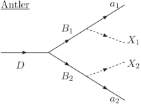
Figure 1: The antler decay topology of a heavy new particle $D$ into two missing particles ($X_{1}$ and $X_{2}$) and two visible particles ($a_{1}$ and $a_{2}$).

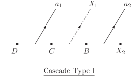
xxx

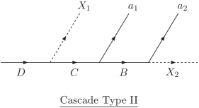
Figure 2: The cascade decay topology of a heavy new particle $D$ into two missing particles ($X_{1}$ and $X_{2}$) and two visible particles ($a_{1}$ and $a_{2}$).

Recently, it has been pointed out that the missing particle mass can be determined from singular structures in kinematic distributions for shorter and simpler decay chains cusp ; Kim:2009si . In our previous work cusp , we considered a resonant “antler decay” of a heavy new particle into a pair of missing particles and a pair of SM visible particles, as shown in Fig. 1, and found non-smooth peaks in some kinematic distributions. These peaks are called “cusps” and the positions of the cusps depend only on the masses of the involved particles. The cusp is statistically more advantageous because it is at the peak region. The mass measurements can be benefited from knowing the kinematic cusp structures.

We consider a resonant decay of a heavy particle $D$ into two visible particles and two missing particles. The invariant mass distributions of this type of decay were first presented in our previous publication cusp , and recently further studied in Ref. Invariant:mass . Obviously this heavy particle $D$ is parity-even. The general topology of such resonance decays is divided into two classes:

1. Antler decay topology: a heavy particle $D$ decays into two parity-odd particles ($B_{1}$ and $B_{2}$) at the first step and each parity-odd particle subsequently decays into a missing (denoted by dashed lines) particle and a visible particle, as in Fig. 1.

2. Cascade decay topology: a heavy particle $D$ splits to two particles with one or both visible particles at each step, finally into a missing particle. According to at which step the first missing particle comes out, there are two non-trivial cascade topologies, as in Fig. 2.

The antler decay and the cascade decay are siblings to each other as they share the same skeleton of topology. Since they have different orientation of incoming and outgoing particles, the cusps appear with different manifestations. In this paper, we focus on the antler topology only and leave the presentation on the cascade decay topology to a companion paper long:cascade .

Antler decays arise in many new physics models. We now list a few examples for illustration.

• In the Minimal Supersymmetric Standard Model (MSSM), the heavy CP-even neutral Higgs bosons may have sizable rates of the following decay Higgs:MSSM :

  $$H\rightarrow{\tilde{\chi}^{0}_{2}}+{\tilde{\chi}^{0}_{2}}\rightarrow Z{\tilde{\chi}^{0}_{1}}+Z{\tilde{\chi}^{0}_{1}}.$$ (1)

• In the MSSM with an additional $U(1)$ gauge interaction, the extra $U(1)$ gauge boson $Z^{\prime}$ can have antler decay modes like Zp

  $$Z^{\prime}\rightarrow\tilde{\ell}^{-}+\tilde{\ell}^{+}\rightarrow\ell^{-}{\tilde{\chi}^{0}_{1}}+\ell^{+}{\tilde{\chi}^{0}_{1}}.$$ (2)

• The ultraviolet completion of the LHT model often involves an extension of the Higgs sector that accommodates heavy Higgs bosons. Large top Yukawa coupling leads to substantial decay of the neutral heavy Higgs into a pair of $T$-parity odd top quarks $t_{-}$, followed by $t_{-}$ decay into the SM top quark and the heavy photon $A_{H}$ (the CDM candidate) DMLittleHiggs :

  $$H\rightarrow t_{-}+\bar{t}_{-}\rightarrow tA_{H}+\bar{t}A_{H}.$$ (3)

• In the UED model with KK parity conservation, the second KK mode of the $Z$ boson can have antler decay modes KK2:mUED . $Z^{(2)}$ decays into a pair of the first KK modes of the lepton, followed by its decay into a SM lepton and the CDM particle $B^{(1)}$:

  $$Z^{(2)}\rightarrow L^{(1)}+L^{(1)}\rightarrow\ell^{-}B^{(1)}+\ell^{+}B^{(1)}.$$ (4)

• At lepton colliders with $e^{+}e^{-}$ or $\mu^{+}\mu^{-}$ collisions, the well-determined c.m. energy renders some pair production and their subsequent decay processes to be of the antler topology. One example is

  $$e^{+}e^{-}/\mu^{+}\mu^{-}\to\tilde{\ell}^{+}+\tilde{\ell}^{-}\to\ell^{+}{\tilde{\chi}^{0}_{1}}+\ell^{-}{\tilde{\chi}^{0}_{1}}.$$ (5)

In the current work, we only focus on the generic features of antler kinematics. The rest of the paper is organized as follows. We begin our discussion by explaining the unique features of the antler kinematics in Sec. II. Focused on the symmetric antler decay, we consider the massive visible particle case, and demonstrate in Sec. III the cusps and endpoints in the kinematic distributions of the invariant mass, transverse momenta, and angular variables, constructed from two visible particles. In Sec. IV, we study the massless visible particle case. We discuss some effects of more realistic considerations in Sec. V, such as the finite decay widths of the resonant particles, the longitudinal boost between the c.m. frame and the lab frame, and spin correlations. We conclude in Sec. VI. A few appendices are devoted to some technical details for a general four-body phase space treatment, the derivations of the cusp peak and analytic expressions of some kinematic distribution, and more discussions for the general antler decay.

II Kinematics of antler decay topology with two missing particles

We consider the resonant decay of a heavy particle $D$ into two visible particle $a_{1}$ and $a_{2}$, and two missing particle $X_{1}$ and $X_{2}$ via a chain of two-body decays through intermediate particles $B_{1}$ and $B_{2}$, as depicted in Fig. 1:

$$D(P) \to B_{1}(p_{1})+B_{2}(p_{2}),$$

$$B_{1}(p_{1})\to a_{1}(k_{1})+X_{1}(k_{3}),\quad B_{2}(p_{2})\to a_{2}(k_{2})+X_{2}(k_{4}).$$

Since most of the processes of our interest are symmetric between two decay branches, we focus on the symmetric antler decay, defined by

$$\hbox{Symmetric antler: }B\equiv B_{1}=B_{2},\quad a\equiv a_{1}=a_{2},\quad X\equiv X_{1}=X_{2}.$$ (7)

The general antler decay with arbitrary masses is to be discussed in Appendix B.

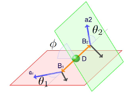
Figure 3: Kinematic configuration of the antler decay in the rest frame of the parent particle $D$ via two intermediate particles $B_{1}$ and $B_{2}$, followed by $B\to aX$. $\theta_{1}$ and $\theta_{2}$ are defined in the rest frames of $B_{1}$ and $B_{2}$, respectively, and $\phi$ in the $D$ rest frame.

In the three-dimensional momentum space, the kinematic configuration of the antler decay is illustrated in Fig. 3. In the rest frame of the parent particle $D$, the intermediate particles $B_{1}$ and $B_{2}$ are moving back-to-back, and the momentum direction defines the principal decay axis $z$, with $B_{1}$ moving into the $+z$ direction and $B_{2}$ into the $-z$ direction. Two momenta of $a_{1}$ and $X_{1}$ in the $B_{1}$ rest frame form the decay plane $P1$, which is identified as the $xz$-plane. In the same way, the decay plane $P2$ is defined by the $B_{2}$ decay products. In the decay plane $P1$, we define a polar angle $\theta_{1}$ between the $+z$ direction and the $a_{1}$ momentum in the $B_{1}$ rest frame. Similarly, $\theta_{2}$ is the polar angle between the $-z$ direction and the $a_{2}$ momentum in the $B_{2}$ rest frame. The azimuthal angle between two decay planes $P1$ and $P2$ is denoted by $\phi$.

As explicitly shown in Appendix A, these three internal angles ($\theta_{1}$, $\theta_{2}$, and $\phi$) represent the phase space configuration of the antler decay topology. The dynamics of the antler decay is encoded in the differential decay width $d\Gamma$ defined in the rest frame of $D$. $d\Gamma$ is a function of the internal phase space variable $(\theta_{1},\theta_{2},\phi)$:

$$d{\Gamma}\propto\widehat{|{\mathcal{M}}|^{2}}\,{d\widehat{\Phi}_{4}},$$ (8)

where $\widehat{|{\mathcal{M}}|^{2}}$ is a reduced matrix elements and ${d\widehat{\Phi}_{4}}=d\cos\theta_{1}\,d\cos\theta_{2}\,d\phi$ (see Appendix A for more details). The reduced matrix element $\widehat{|{\mathcal{M}}|^{2}}$ is a smooth function of $(\theta_{1},\theta_{2},\phi)$, and thus $d\Gamma/{d\widehat{\Phi}_{4}}$ does not show any singular behavior.

Kinematic singularities emerge as missing particles allow us only the projection of the full kinematic phase space onto a lower dimensional phase space accessible by the visible particle momenta. This partial access inevitably hides some of necessary information for the full mass reconstruction. However, we can still decode the mass information out of some observables, say $Y$’s.

In order to obtain $d\Gamma/dY$, we project the hypersurface of the phase space $(\theta_{1},\theta_{2},\phi)$ onto $Y$: for each value of $Y$, $d{\Gamma}/dY$ is proportional to the volume of the hypersurface corresponding to that specific value of $Y$. When the hypersurface fails to be a manifold at a certain point $Y$, $d{\Gamma}/dY$ develops non-smoothness. This is called singular points, where the differential $(\partial Y/\partial\theta_{1},\partial Y/\partial\theta_{2},\partial Y/\partial\phi)$ vanishes . As a result, we see non-smooth behaviors in the distribution of $Y$, which give rise to kinematic cusps and endpoints. General discussions on the development of singularity in the multi-dimensional observable phase space have been presented in Ref. Kim:2009si .

Since the parent particle $D$ is moving in the lab frame, the observable variable $Y$ from the momenta of two visible particles $a_{1}$ and $a_{2}$ can be classified into three categories:

• Lorentz-invariant observable: there is only one Lorentz-invariant observable, the invariant mass of $a_{1}$ and $a_{2}$,

  $$m=\sqrt{(k_{1}+k_{2})^{2}}.$$ (9)

• Longitudinal-boost invariant observables:

  • the transverse momentum of one visible particle $i$:

    $$p_{Ti}=\left|\mathbf{k}_{iT}\right|.$$ (10)

    Here and henceforth, a bold-faced letter denotes a three-momentum.

  • the total transverse momentum of the $a_{1}$-$a_{2}$ system:

    $$p_{T}=\left|\mathbf{k}_{1T}+\mathbf{k}_{2T}\right|.$$ (11)

    In the four-body decay under consideration, this is the same as the magnitude of the missing transverse momentum ${\hbox to0.0pt{/\hss}p_{T}}$ of the decay.

  • the transverse mass of the $a_{1}$-$a_{2}$ system:

    $$m_{T}=\sqrt{p_{T}^{2}+m^{2}}.$$ (12)

  • the cluster transverse mass of the $a_{1}$-$a_{2}$-$\,{\hbox to0.0pt{/\hss}p_{T}}$ system:

    $$m_{T}^{C}=m_{T}+{\hbox to0.0pt{/\hss}p_{T}}.$$ (13)

  • the rapidity difference:

    $$\Delta\eta=|\eta_{a1}-\eta_{a2}|,\quad{\rm where}\ \ \eta_{ai}={1\over 2}\ln\left({{E_{i}+k_{iz}}\over{E_{i}-k_{iz}}}\right).$$ (14)

• Non-invariant observable: we consider an angular variable $\Theta$, which is the angle between one visible particle (say $a_{1}$) in the c.m. frame of $a_{1}$ and $a_{2}$ and the c.m. moving direction in the $D$ rest frame, given by

  $$\cos\Theta=-\frac{\mathbf{k}_{1}^{(a_{1}a_{2})}\cdot(\mathbf{k}_{1}+\mathbf{k}_{2})^{(D)}}{\big{|}\mathbf{k}_{1}^{(a_{1}a_{2})}\big{|}~{}\big{|}\mathbf{k}_{1}+\mathbf{k}_{2}\big{|}^{(D)}}.$$ (15)

  In what follows, the superscript in a momentum denotes the reference frame. In the main text, a momentum without a superscript is in the lab frame.

III Massive visible particle case

In this section, we consider the case of massive visible particles. For a resonant decay, it is very convenient to express the kinematics in terms of rapidity variables. For a two-body decay of $i\rightarrow j+k$, we write the four-momentum of the particle $j$ in the rest frame of the parent particle $i$ as $p_{j}^{(i)}=(E_{j}^{(i)},\mathbf{p}_{j}^{(i)})=(m_{j}\cosh\eta_{j},m_{j}\sinh\eta_{j}\hat{\mathbf{p}}^{(i)}_{j})$. Here $\eta_{j}$ is the rapidity of particle $j$ in the rest frame of the parent $i$, given by

$$\cosh\eta_{j}\equiv{E_{j}^{(i)}\over m_{j}}=\frac{m_{i}^{2}+m_{j}^{2}-m_{k}^{2}}{2m_{i}m_{j}}.\\$$ (16)

The superscript of a rapidity, specifying the reference frame, is omitted when it is the rest frame of the parent particle. In this section, we assume that all the particles are massive. The massless case will be covered in the next session by taking the massless limit from the massive case.

Now we illustrate the symmetric antler decay defined in Eq. (7), which has two independent rapidity parameters $\eta_{B}$ and $\eta_{a}$:

$$\cosh\eta_{B}=\frac{m_{D}}{2m_{B}},\quad\cosh\eta_{a}=\frac{m_{B}^{2}-m_{X}^{2}+m_{a}^{2}}{2m_{a}m_{B}}.$$ (17)

Note that $\eta_{B}$ is determined from $D\rightarrow B_{1}B_{2}$ decay, and $\eta_{a}$ from $B_{1}\rightarrow a_{1}X_{1}$ decay (or $B_{2}\rightarrow a_{2}X_{2}$ equivalently).

In the $D$ rest frame, the momenta of the particles $a_{1}$ and $a_{2}$ are

$$k^{(D)}_{1} = m_{a}\left(\begin{array}[]{c}\cosh\eta_{B}\cosh\eta_{a}+\sinh\eta_{B}\sinh\eta_{a}\cos\theta_{1}\\ \sinh\eta_{a}\sin\theta_{1}\\ 0\\ \sinh\eta_{B}\cosh\eta_{a}+\cosh\eta_{B}\sinh\eta_{a}\cos\theta_{1}\end{array}\right),$$ (22)

$$k^{(D)}_{2} = m_{a}\left(\begin{array}[]{c}\cosh\eta_{B}\cosh\eta_{a}+\sinh\eta_{B}\sinh\eta_{a}\cos\theta_{2}\\ \sinh\eta_{a}\sin\theta_{2}\cos\phi\\ \sinh\eta_{a}\sin\theta_{2}\sin\phi\\ -\sinh\eta_{B}\cosh\eta_{a}-\cosh\eta_{B}\sinh\eta_{a}\cos\theta_{2}\end{array}\right),$$ (27)

where the internal phase space angles of $(\theta_{1},\theta_{2},\phi)$ are defined in Fig. 3.

III.1 Invariant mass distribution

The invariant mass of the two visible particles $a_{1}$ and $a_{2}$ is explicitly obtained from $k^{(D)}_{1}$ and $k^{(D)}_{2}$ in Eqs. (22) and (27):

$$m^{2} = m_{a}^{2}\bigg{[}\left\{2\cosh\eta_{B}\cosh\eta_{a}+\sinh\eta_{B}\sinh\eta_{a}(\cos\theta_{1}+\cos\theta_{2})\right\}^{2}$$ (28)

$$\qquad-\sinh^{2}\eta_{a}(\sin\theta_{1}+\sin\theta_{2}\cos\phi)^{2}-\sinh^{2}\eta_{a}\sin^{2}\theta_{2}\sin^{2}\phi$$

$$\qquad-\cosh^{2}\eta_{B}\sinh^{2}\eta_{a}(\cos\theta_{1}-\cos\theta_{2})^{2}\bigg{]}\,.$$

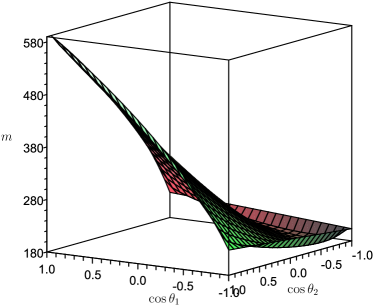
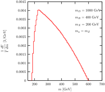
Figure 4: (a) The invariant mass $m$ as a function of $\cos\theta_{1}$ and $\cos\theta_{2}$, with $\phi=0$. (b) The normalized differential decay rate as a function of $m$. We take the mass parameters of $m_{D}=1{\,{\rm TeV}}$, $m_{B}=400{\,{\rm GeV}}$, $m_{X}=200{\,{\rm GeV}}$ and $m_{a}=m_{Z}$.

In Fig. 4(a), we show the invariant mass $m$ as a function of $\cos\theta_{1}$ and $\cos\theta_{2}$. For the sake of illustration, we take $m_{D}=1{\,{\rm TeV}},\ m_{B}=400{\,{\rm GeV}},\ m_{a}=m_{Z},\ m_{X}=200{\,{\rm GeV}}$, and fixed $\phi=0$. The mapping of this non-trivial hypersurface onto the $m$ yields a singular structure in the $d\Gamma/dm$ distribution as in Fig. 4(b). To understand how this distinctive feature occurs, we study this mapping by examining the following some critical points:

• Point (i): $(\cos\theta_{1},\cos\theta_{2})=(1,1)$
  Since $a_{1}$ and $a_{2}$ move back-to-back in the $D$ rest frame, their invariant mass becomes maximum. The rapidity of $a_{1}$ in the rest frame of $D$ is the same as that of $a_{2}$, such that $|\eta_{a_{1}}^{(D)}|=|\eta_{a_{2}}^{(D)}|=\eta_{B}+\eta_{a}$. Therefore, the relative rapidity of $a_{2}$ with respect to $a_{1}$ is $\eta^{(a_{1})}_{a_{2}}=2(\eta_{B}+\eta_{a})$.

• Point (ii): $(\cos\theta_{1},\cos\theta_{2})=(\pm 1,\mp 1)$
  One visible particle, say $a_{1}$, moves in the same direction of its parent $B_{1}$ with the rapidity of $\eta^{(D)}_{a_{1}}=\eta_{B}+\eta_{a}$, and the other visible particle $a_{2}$ moves in the opposite direction of its parent with $\eta^{(D)}_{a_{2}}=|\eta_{B}-\eta_{a}|$. If $\eta_{a}>\eta_{B}$, the directions of $a_{1}$ and $a_{2}$ in the $D$ rest frame are the same, which implies $\eta^{(a_{1})}_{a_{2}}=\eta^{(D)}_{a_{1}}-\eta^{(D)}_{a_{2}}$. If $\eta_{a}<\eta_{B}$, the direction of $a_{1}$ and $a_{2}$ are opposite so that $\eta^{(a_{1})}_{a_{2}}=\eta^{(D)}_{a_{1}}+\eta^{(D)}_{a_{2}}$. Therefore, regardless of the ordering of $\eta_{a}$ and $\eta_{B}$, $\eta^{(a_{1})}_{a_{2}}=2\eta_{B}$. Note that two configurations of $(\cos\theta_{1},\cos\theta_{2})=(1,-1)$ and $(\cos\theta_{1},\cos\theta_{2})=(-1,1)$ are symmetric to each other.

• Point (iii): $(\cos\theta_{1},\cos\theta_{2})=(-1,-1)$
  $a_{1}$ and $a_{2}$ move in the opposite direction to $B_{1}$ and $B_{2}$ in their parent’s rest frames, respectively. Their rapidities are $|\eta_{a_{1}}^{(D)}|=|\eta_{a_{2}}^{(D)}|=|\eta_{B}-\eta_{a}|$, leading to $\eta^{(a_{1})}_{a_{2}}=2|\eta_{B}-\eta_{a}|$.

• Point (iv): $\theta_{2}=\theta_{1},\ \phi=0,\ \cos\theta_{1}=-\tanh\eta_{B}/\tanh\eta_{a}$ with $\eta_{a}>\eta_{B}$
  This special configuration gives rise to the same four-momenta of the two visible particles as can be seen in Eqs. (22) and (27). $a_{1}$ and $a_{2}$ are relatively at rest, resulting in $\eta^{(a_{1})}_{a_{2}}=0$. The condition $\eta_{a}>\eta_{B}$ is required to guarantee the equality of $k_{1}^{(D)}$ and $k_{2}^{(D)}$, which cannot be achieved if the particle $B$ is boosted more highly than the particle $a$ (or equivalently $|\cos\theta_{1}|\leq 1$ for physical configurations).

Point (i) corresponds to the maximum endpoint, and Points (ii) to the cusped peak. When Point (iv) exists, Point (iii) corresponds to the non-smooth kink, and Point (iv) to the minimum endpoint at $m=2m_{a}$. Otherwise, Point (iii) becomes the minimum endpoint at $m=2m_{a}\cosh(\eta_{B}-\eta_{a})$.

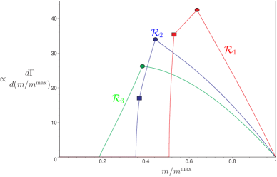
Figure 5: The shapes of the function of $d\Gamma/dm$ for three representative regions, ${\mathcal{R}}_{1}$, ${\mathcal{R}}_{2}$, and ${\mathcal{R}}_{3}$. With the fixed ${\eta_{a}}=1$, we set $\eta_{B}=0.3$ for ${\mathcal{R}}_{1}$, $\eta_{B}=0.7$ for ${\mathcal{R}}_{2}$, and $\eta_{B}=1.5$ for ${\mathcal{R}}_{3}$.

Now we present the analytic expression of the invariant mass distribution. The functional forms are different in the following three mass regions:

$${\mathcal{R}}_{1}:\eta_{B}<\frac{{\eta_{a}}}{2},\qquad{\mathcal{R}}_{2}:\frac{{\eta_{a}}}{2}<\eta_{B}<{\eta_{a}},\qquad{\mathcal{R}}_{3}:{\eta_{a}}<\eta_{B}.$$ (29)

In Fig. 5, we show the invariant mass distribution $d\Gamma/d(m/m_{\rm max})$ for ${\mathcal{R}}_{1}$, ${\mathcal{R}}_{2}$, and ${\mathcal{R}}_{3}$. Regardless of the parameter regions, the maximum endpoint of the $m$ distribution corresponds to Point (i):

$$m_{\rm max}=2m_{a}\cosh(\eta_{B}+\eta_{a}).$$ (30)

For ${\mathcal{R}}_{1}$ and ${\mathcal{R}}_{2}$, the minimum endpoint occurs at $m=2m_{a}$ while for ${\mathcal{R}}_{3}$ the minimum is different:

$$m_{\rm min}=\begin{cases}\begin{array}[]{ll}2m_{a},&\mbox{ for ${\mathcal{R}}_{1}$ and ${\mathcal{R}}_{2}$},\\ 2m_{a}\cosh(\eta_{B}-\eta_{a}),&\mbox{ for ${\mathcal{R}}_{3}$}.\end{array}\end{cases}$$ (31)

The condition of $\eta_{B}>\eta_{a}$ in ${\mathcal{R}}_{3}$ does not allow the equality of $k_{1}^{(D)}=k_{2}^{(D)}$ which would lead to $m_{\rm min}=2m_{a}$. In ${\mathcal{R}}_{1}$ and ${\mathcal{R}}_{2}$, there are two non-smooth points in the middle of the distribution. Let us call the point at the smaller value of $m$ (marked by squares) a knee point and the other point at the larger value of $m$ (marked by circles) a cusp point. In ${\mathcal{R}}_{1}$, the knee point corresponds to Point (ii) and the cusp point to Point (iii). In ${\mathcal{R}}_{2}$, it is opposite. In ${\mathcal{R}}_{3}$, there is only one sharp peak, the cusp. We summarize the results of the minimum, cusp, knee, and maximum of the $m$ distribution in Table 1.

	$~{}~{}~{}{\mathcal{R}}_{1}$	$~{}~{}~{}{\mathcal{R}}_{2}$	$~{}~{}~{}{\mathcal{R}}_{3}$
$m_{\rm min}$	$2m_{a}$	$2m_{a}$	$2m_{a}{c}_{\eta_{B}-{\eta_{a}}}$
$m_{\rm knee}$	$2m_{a}c_{\eta_{B}}$	$2m_{a}c_{\eta_{B}-\eta_{a}}$	-
$m_{\rm cusp}$	$2m_{a}{c}_{\eta_{B}-{\eta_{a}}}$	$2m_{a}{c}_{\eta_{B}}$	$2m_{a}{c}_{\eta_{B}}$
$m_{\rm max}$	$2m_{a}c_{\eta_{B}+\eta_{a}}$	$2m_{a}c_{\eta_{B}+\eta_{a}}$	$2m_{a}c_{\eta_{B}+\eta_{a}}$

Table 1: Summary of the minimum, cusp, knee, and maximum of the $m$ distribution for the mass parameter regions ${\mathcal{R}}_{1}$, ${\mathcal{R}}_{2}$, and $R_{3}$. We have used a concise notation of $\cosh x\equiv c_{x}$.

The invariant mass distributions for three mass regions are

$$\left.\frac{d\Gamma}{dm}\right|_{{\mathcal{R}}_{1}}\!\!\! \propto \left\{\begin{array}[]{ll}2m\cosh^{-1}\left(\frac{m^{2}}{2m_{a}^{2}}-1\right),&\hbox{ if }~{}2m_{a}<m<2m_{a}c_{\eta_{B}};\\ 4\eta_{B}\,m,&\hbox{ if }~{}2m_{a}c_{\eta_{B}}<m<2m_{a}c_{{\eta_{B}}-{\eta_{a}}};\\ m\left[2(\eta_{B}+{\eta_{a}})-\cosh^{-1}\left(\frac{m^{2}}{2m_{a}^{2}}-1\right)\right],&\hbox{ if }~{}2m_{a}c_{{\eta_{B}}-{\eta_{a}}}<m2m_{a}c_{{\eta_{B}}+{\eta_{a}}};\\ 0,&\hbox{ otherwise },\end{array}\right.$$ (36)

$$\left.\frac{d\Gamma}{dm}\right|_{{\mathcal{R}}_{2}}\!\!\! \propto \left\{\begin{array}[]{ll}2m\cosh^{-1}\left(\frac{m^{2}}{2m_{a}^{2}}-1\right),&\hbox{ if }~{}2m_{a}<m2m_{a}c_{{\eta_{B}}-{\eta_{a}}};\\ m\left[2({\eta_{a}}-\eta_{B})+\cosh^{-1}\left(\frac{m^{2}}{2m_{a}^{2}}-1\right)\right],&\hbox{ if }~{}2m_{a}c_{{\eta_{B}}-{\eta_{a}}}<m2m_{a}c_{\eta_{B}};\\[5.69046pt] m\left[2({\eta_{a}}+\eta_{B})-\cosh^{-1}\left(\frac{m^{2}}{2m_{a}^{2}}-1\right)\right],&\hbox{ if }~{}2m_{a}c_{{\eta_{B}}}<m<2m_{a}c_{{\eta_{B}}+{\eta_{a}}},\\ 0,&\hbox{ otherwise },\end{array}\right.$$ (41)

$$\left.\frac{d\Gamma}{dm}\right|_{{\mathcal{R}}_{3}}\!\!\! \propto \left\{\begin{array}[]{ll}m\left[2{\eta_{a}}-2\eta_{B}+\cosh^{-1}\left(\frac{m^{2}}{2m_{a}^{2}}-1\right)\right],&\hbox{ if }~{}2m_{a}c_{{\eta_{B}}-{\eta_{a}}}<m<2m_{a}c_{\eta_{B}};\\[5.69046pt] m\left[2{\eta_{a}}+2\eta_{B}-\cosh^{-1}\left(\frac{m^{2}}{2m_{a}^{2}}-1\right)\right],&\hbox{ if }~{}2m_{a}c_{\eta_{B}}<m<2m_{a}c_{{\eta_{B}}+{\eta_{a}}};\\ 0,&\hbox{ otherwise }.\end{array}\right.$$ (45)

Here we have employed the narrow width approximation and ignored spin correlation effects. The detailed derivation is presented in Appendix A.

	Region	$m_{D}$	$m_{B}$	$m_{a}$	$m_{X}$	$\eta_{B}$	${\eta_{a}}$
Mass–1	${\mathcal{R}}_{1}$	650	300	$m_{Z}$	100	0.41	1.06
Mass–2	${\mathcal{R}}_{2}$	850	330	$m_{Z}$	100	0.74	1.18
Mass–3	${\mathcal{R}}_{3}$	1000	250	$m_{Z}$	100	1.32	0.80

Table 2: Test mass spectrum sets for the symmetric antler decay. All masses are in units of GeV and $m_{Z}$ is the $Z$ boson mass. $\eta_{B}$ and $\eta_{a}$ are the rapidities of the particle $B$ and $a$ in its parent rest frame, respectively.

In order to show the characteristics of the $m$ distribution, we take three samples for mass parameters in Table 2. We label them as Mass–1, Mass–2 and Mass–3, each of which corresponds to the kinematical regions of ${\mathcal{R}}_{1}$, ${\mathcal{R}}_{2}$ and ${\mathcal{R}}_{3}$, respectively. The visible particle is assumed to be the $Z$ boson.

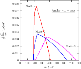
Figure 6: The normalized invariant mass distribution $d{\Gamma}/dm$ for test mass sets in Table 2.

In Fig. 6, we present the invariant mass distributions for the mass parameters in Table 2. All three mass sets yield sharp cusp structures. The $m$ minimum for ${\mathcal{R}}_{1}$ and ${\mathcal{R}}_{2}$ is $2m_{Z}$ as discussed before. For the ${\mathcal{R}}_{3}$ case, however, fast-moving intermediate particle $B$ yields $m_{\rm min}=2m_{Z}\cosh(\eta_{B}-\eta_{a})$. Unfortunately, we still have a two-fold ambiguity between ${\mathcal{R}}_{1}$ and ${\mathcal{R}}_{2}$ because we do not know a priori whether the observed $m_{\rm cusp}$ is $2m_{a}\cosh(\eta_{B}-\eta_{a})$ or $2m_{a}\cosh\eta_{B}$. As shall be shown in the next section, the transverse momentum distribution breaks this ambiguity through its cusp and endpoint structures. In addition, the ${\mathcal{R}}_{1}$ and ${\mathcal{R}}_{2}$ cases have the knee structure, even though it is challenging to probe with the expected statistics at the LHC.

III.2 Transverse momentum variables: $m_{T}$, $p_{T}$, and $p_{Ti}$

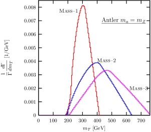
Figure 7: The normalized transverse mass distribution $d{\Gamma}/dm_{T}$ for test mass sets in Table 2.

In this section, we investigate the distribution of the transverse mass $m_{T}$, the transverse momentum variables $p_{T}$ and $p_{Ti}$. In Fig. 7, we show the $m_{T}$ distribution. All the $m_{T}$ distributions for ${\mathcal{R}}_{1}$, ${\mathcal{R}}_{2}$, and ${\mathcal{R}}_{3}$ do not have any cusped peak. The maximum in the $m_{T}$ distribution is the same as the maximum of $m$:

$$\left(m_{T}\right)_{\rm max}=m_{\rm max}.$$ (46)

The confirmation of the same maxima in the $m$ and $m_{T}$ distributions will help the reconstruction of the antler decay.

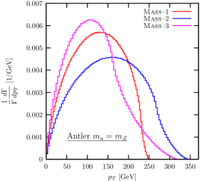
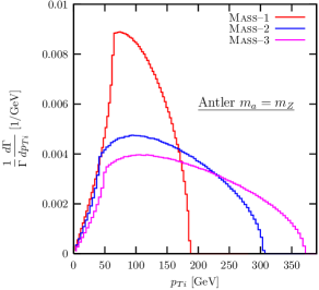
Figure 8: The normalized transverse momentum distribution $d{\Gamma}/dp_{T}$ and $d\Gamma/dp_{Ti}$ for test mass sets in Table 2.

In Fig. 8, we plot the distribution of $p_{T}$ and $p_{Ti}$. The total $p_{T}$ distribution does not reveal the cusp structure, as expected from the $m_{T}$ distribution. In addition, its maximum is at the end of a long tail, which is statistically disadvantageous to observe. The cluster transfer mass $m_{C}$ of $a_{1}$-$a_{2}$-$\,{\hbox to0.0pt{/\hss}p_{T}}$ system has no cusp structure either.

The transverse momentum of “one” visible particle shows quite different distribution. First, note that one unambiguous $p_{Ti}$ distribution can be constructed out of two visible particles, because of the symmetric topology of the antler decay. This $p_{Ti}$ distribution shows the cusp structure as well as the fast-dropping maximum structure. The cusp and maximum of $p_{Ti}$ are

$$\left(p_{Ti}\right)_{\rm cusp} = m_{a}\left|\sinh({\eta_{a}}-\eta_{B})\right|,$$ (47)

$${}\left(p_{Ti}\right)_{\rm max} = m_{a}\sinh\left(\eta_{a}+{\eta_{B}}\right).$$

Note that $\left(p_{Ti}\right)_{\rm max}$ gives the information about $\eta_{B}+\eta_{a}$, which is the same from $m_{\rm max}$ in Eq. (30). Remarkable is that $\left(p_{Ti}\right)_{\rm cusp}$ is common for all three regions ${\mathcal{R}}_{1,2,3}$, which determines $|\eta_{B}-\eta_{a}|$. By comparing $(p_{Ti})_{\rm cusp}$ with $m_{\rm cusp}$, we can distinguish ${\mathcal{R}}_{1}$ from ${\mathcal{R}}_{2}$. This breaks the two-fold ambiguity in the measurement of $m_{\rm cusp}$ for ${\mathcal{R}}_{1}$ and ${\mathcal{R}}_{2}$.

III.3 Angular variable: $\cos\Theta$

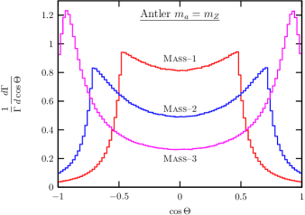
Figure 9: The normalized $\cos{\Theta}$ distribution for the massive visible particle cases.

We consider the distribution of $\cos\Theta$ defined in Eq. (15). Here $\Theta$ is the angle of one visible particle with respect to the c.m. moving direction. As in the $p_{Ti}$ distribution, the symmetric decay chains of the antler decay guarantee one unique $\cos{\Theta}$ distribution as shown in Fig. 9. All $\cos\Theta$ distributions for ${\mathcal{R}}_{1}$, ${\mathcal{R}}_{2}$ and ${\mathcal{R}}_{3}$ are symmetric about $\cos\Theta=0$, and have sharp cusps.

IV Massless visible particle case

Now we consider the massless visible particle case. As suggested in Eqs. (2), (4), and (5), many new physics processes for the antler decay have massless visible particles. Although we cannot directly apply the results with the massive visible particle to this case since the rapidity $\eta_{a}$ diverges, we can obtain the massless limit by using the finite combinations of $m_{a}c_{\eta_{a}}$ and $m_{a}s_{\eta_{a}}$:

$$\lim_{m_{a}\to 0}m_{a}c_{\eta_{a}} = \lim_{m_{a}\to 0}m_{a}s_{\eta_{a}}=\frac{m_{B}}{2}\left(1-\frac{m_{X}^{2}}{m_{B}^{2}}\right).$$ (48)

IV.1 Invariant mass distribution

In the massive visible particle case, the functional form of the invariant mass distribution is different according to three mass regions of ${{\mathcal{R}}_{1}}$, ${{\mathcal{R}}_{2}}$, and ${{\mathcal{R}}_{3}}$. In the massless visible particle case, only ${\mathcal{R}}_{1}$ applies since $\eta_{B}\ll\eta_{a}$. Two locations of $m_{\rm min}$ and $m_{\rm knee}$ merge because $m_{a}=0$. The cusp and endpoints are given by

$$m_{\rm min}^{(0)} = 0,$$ (49)

$$m_{\rm cusp}^{(0)} = m_{B}\left(1-\frac{m_{X}^{2}}{m_{B}^{2}}\right)e^{-\eta_{B}},$$ (50)

$$m_{\rm max}^{(0)} = m_{B}\left(1-\frac{m_{X}^{2}}{m_{B}^{2}}\right)e^{\eta_{B}}.$$ (51)

Here the superscript $(0)$ is used for emphasizing $m_{a}=0$. The product of the cusp and the maximum is

$$m_{\rm cusp}^{(0)}m_{\rm max}^{(0)}={m_{B}^{2}}\left(1-\frac{{m_{X}^{2}}}{m_{B}^{2}}\right)^{2},$$ (52)

which depends only on the second step decay of $B\to aX$. The ratio is

$$\frac{m_{\rm cusp}^{(0)}}{m_{\rm max}^{(0)}}=e^{-2\eta_{B}},$$ (53)

which is determined only by the first step decay of $D\to BB$.

The invariant mass distribution is simplified into

$$\frac{d\Gamma}{dm}\propto\begin{cases}\begin{array}[]{ll}m\log\left(\frac{m_{\rm max}^{(0)}}{m_{\rm cusp}^{(0)}}\right),&\mbox{ if $0<m<m_{\rm cusp}^{(0)}$; }\\ m\log\left(\frac{m_{\rm max}^{(0)}}{m}\right),&\mbox{ if $m_{\rm cusp}^{(0)}<m<m_{\rm max}^{(0)}$;}\\ 0,&\mbox{ otherwise. }\end{array}\end{cases}$$ (54)

For $0<m<m_{\rm cusp}^{(0)}$, $d\Gamma/dm$ is a linear function of $m$. For $m_{\rm cusp}^{(0)}<m<m_{\rm max}^{(0)}$, it is a concave function with the maximum at $m=m_{\rm max}^{(0)}/e$. Depending on the relative position of $m_{\rm cusp}^{(0)}$ and $m_{\rm max}^{(0)}/e$, the maximum of the concave function may or may not show in the function of $d{\Gamma}/dm$, which determines the sharpness of the cusp. If $m_{\rm max}^{(0)}/e<m_{\rm cusp}^{(0)}$ (or equivalently $m_{B}>0.443\,m_{D}$), $d{\Gamma}/dm$ is linearly increasing up to $m=m_{\rm cusp}^{(0)}$, and decreasing after that: the cusp is sharp. If $m_{\rm cusp}^{(0)}<m_{\rm max}^{(0)}/e$, $d{\Gamma}/dm$ keeps increasing after $m=m_{\rm cusp}^{(0)}$, reaches the maximum of the concave function, and finally falls down: the cusp is not sharp. The $m$ cusp structure is most useful when the $D\to BB$ decay is near the threshold.

	$m_{D}$	$m_{B}$	$m_{X}$	$m_{a}$	$m_{\rm cusp}^{(0)}$	$m_{\rm max}^{(0)}$	$|\cos{\Theta}|_{\rm max}$
Mass–10	1000	470	440	0	40.7	82.9	0.34
Mass–20	1000	440	410	0	34.6	97.1	0.47
Mass–30	1000	400	370	0	28.9	115.5	0.60

Table 3: Test mass spectrum sets for the symmetric antler decay with massless SM particles. All masses are in units of GeV.

In order to show the functional behaviors specifically, we take three mass sets for the massless visible particle case in Table 3. The mass parameters in the Mass–1₀ correspond to the case where both the first decay $D\to BB$ and the second decay $B\to aX$ occur near the threshold. This is motivated by the decay of the second KK mode of $Z$ boson in the UED model in Eq.(4). The Mass–2₀ represents the marginal case for the sharp cusp, i.e., $m_{B}\approx 0.44\ m_{D}$. The Mass–3₀ case has large mass gaps.

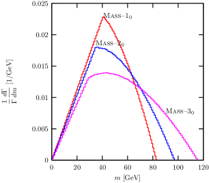
Figure 10: The normalized invariant mass distribution $d{\Gamma}/dm$ in the massless visible particle case for the mass parameter sets in Table 3.

Figure 10 shows the $m$ distributions. All three mass sets in Table 3 have the same $m_{\rm min}=0$. The sharpness of the cusp structure is different. The nearly degenerate mass case (Mass–1₀) has a very sharp cusp. The marginal case (Mass-2₀) shows also an observably sharp cusp. The large mass gap case (Mass-3₀) has a rather smooth cusp. If the number of events is not enough, the obtuse cusp in the Mass-3₀ is difficult to read. The measurement of the $m$ cusp is still possible since the functional form in Eq. (54) can be used to fit the data and to read the cusp position.

IV.2 Transverse momentum variables: $m_{T}$, $p_{T}$ and $p_{Ti}$

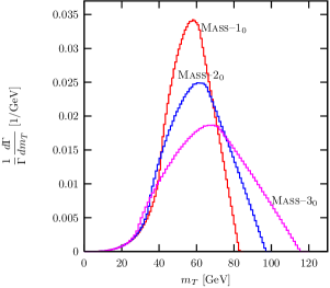
Figure 11: The normalized transverse mass distribution $d{\Gamma}/dm_{T}$ for the massless visible particles. The mass spectrum sets are described in Table 3.

Now we turn to the kinematic variables involving transverse monentum. First, the $m_{T}$ distribution in the massless visible particle case does not show any cusp structure as shown in Fig. 11. The absence of $m_{T}$ cusp is a common feature of the antler decay. The $m_{T}$ maximum stands at the end of fast-dropping function for all three mass sets, which is easier to read. In addition it is the same as the $m$ maximum:

$$(m_{T})_{\rm max}^{(0)}=m_{\rm max}^{(0)}.$$ (55)

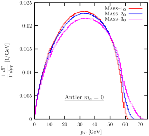
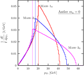
Figure 12: The normalized transverse momentum distribution $d{\Gamma}/dp_{T}$ and $d{\Gamma}/dp_{T_{i}}$ for the massless visible particles. Test mass sets are in Table 3.

Figure 12 shows the distributions of the total transverse momentum $p_{T}$ and individual $p_{Ti}$. As in the massive visible particle case, the total $p_{T}$ distribution is very smooth and gentle, without any cusp structure or fast dropping maximum. Instead, the $p_{Ti}$ distribution shows very sharp cusp, much sharper in general than the invariant mass distribution. Even the Mass–3₀ case, which suffers from the dull cusp in the $m$ distribution, has a very sharp $p_{Ti}$ cusp. In addition the $p_{Ti}$ maximum is at the end of a faster dropping function.

The analytic expressions of $\left(p_{T_{i}}\right)^{(0)}_{\rm cusp}$ and $\left(p_{T_{i}}\right)^{(0)}_{\rm max}$ can be easily obtained from Eq. (47) by applying Eq. (48):

$$\left(p_{Ti}\right)_{\rm cusp}^{(0)}=\frac{1}{2}m_{\rm cusp}^{(0)},\quad\left(p_{Ti}\right)_{\rm max}^{(0)}=\frac{1}{2}m_{\rm max}^{(0)}.$$ (56)

The measurements of $\left(p_{Ti}\right)_{\rm cusp}^{(0)}$ and $\left(p_{Ti}\right)_{\rm max}^{(0)}$ provide the same information as $m_{\rm cusp}^{(0)}$ and $m_{\rm max}^{(0)}$, which is another way to check the antler decay topology.

IV.3 Angular variable: $\cos\Theta$

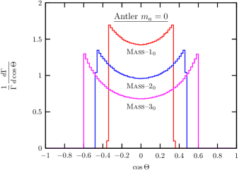
Figure 13: The normalized $\cos{\Theta}$ distribution for the massless visible particle cases.

Figure 13 shows the normalized $d{\Gamma}/d\cos{\Theta}$ distributions for three massless visible particle cases. The function increases with $|\cos{\Theta}|$, and drops to zero suddenly at $\left|\cos{\Theta}\right|^{(0)}_{\rm max}$. This is because the cusp and the endpoint merge, resulting in more pronounced endpoints with sharp peaks at both ends. The maximum of $\cos{\Theta}$ is simply determined by the first step decay $D\to BB$:

$$\left|\cos{\Theta}\right|^{(0)}_{\rm max}=\tanh\eta_{B}.$$ (57)

The full analytic function of ${d\widehat{\Phi}_{4}}/d\cos{\Theta}$ is given by

$$\frac{{\Gamma}}{d\cos{\Theta}}\propto\left\{\begin{array}[]{ll}\dfrac{1}{\sin^{3}{\Theta}},&\hbox{ for }|\cos\Theta|<\tanh\eta_{B},\\ 0,&\hbox{ otherwise. }\end{array}\right.$$ (60)

The suddenly ending behavior of the $\cos\Theta$ distribution is because massless visible particles cannot access all kinematic space of $\cos\Theta$. The detailed derivation of Eqs. (57) and (60) is in Appendix A.4.

V Effects from realistic considerations

In the previous sections, we have considered the kinematics only, ignoring the decay width of the intermediate particle $B$, the longitudinal boost of the parent particle $D$, and the spin correlation. These $S$-matrix element effects can smear the kinematic cusps and endpoints. In the following, we discuss the limitation of determining the missing particle mass using kinematic singularities.

V.1 Finite width effects

The previous results are based on the narrow width approximation. This approach is very effective for the proposed processes in the MSSM, $Z^{\prime}$ supersymmetry, UED, and LHT models since all the intermediate particles ($\tilde{\chi}^{0}_{2}$, $\tilde{\ell}^{\pm}$, $L^{(1)}$, and $t_{-}$) have very small total decay widths, much smaller than one percent of their masses. If the total decay width ${\Gamma}_{B}$ is large, its effects can smear the cusp and endpoint structures. If the on-shell $B$ particle is kinematically not accessible so that the decay process is through off-shell $B$, then the singular structures are destroyed completely since there is no constraints on the phase space from the mass relations.

Figure 14: The invariant mass distribution $d{\Gamma}/dm$ in the antler decay with finite ${\Gamma}_{B}$ effects. We have taken the mass spectrum sets of Mass–1 and Mass–1₀.

In Fig. 14, we show the invariant mass distributions with the effect of finite ${\Gamma}_{B}$ for the massive SM particle case (Mass–1) and the massless case (Mass–1₀). We take ${\Gamma}_{B}$ to be 3%, 10%, and 50% of $m_{B}$ for the massive case, and 1%, 10%, and 50% for the massless case. If ${\Gamma}_{B}/M_{B}$ is small enough ($\leq 3\%$ for the massive case and $\leq 1\%$ for the massless case), the $m$ cusp remains fairly preserved. Even though the sharp cusp gets dull slightly, the position of the cusp is not shifted for both cases. The endpoint position is stable for the massive case, but shifted considerably for the massless case. If ${\Gamma}_{B}/m_{B}$ is about 10%, the cusp is smeared into a round peak and the endpoint position is shifted significantly for both cases. Still the peak of the smeared cusp stands at the same cusp position. If ${\Gamma}_{B}/M_{B}\simeq 50\%$ in which case a large contribution to the $S$-matrix element arises from the intermediate off-shell $B$, the sharpness and position of the cusp are lost. The endpoints move towards new positions of $m=m_{D}-2m_{X}$. This is from the allowed phase space of the decay $D\rightarrow XXaa$. At least we can determine the mass difference between $D$ and $X$ using the $m$ distribution.

Figure 15: The normalized transverse momentum distribution $d{\Gamma}/dp_{T}$ with various finite total decay width of the intermediate particle $B$.

Now we show the ${\Gamma}_{B}$ effects on the $p_{Ti}$ distributions in Fig. 15. We take the massive Mass–1 case and the massless Mass–1₀ case. The $p_{Ti}$ distribution has very vulnerable cusp and endpoint from the finite ${\Gamma}_{B}$ effects. Even for small width effects ($\leq 3\%$ for the massive case and $\leq 1\%$ for the massless case) the sharp cusp becomes dull, and its position is significantly shifted. The $p_{Ti}$ maximum is more sensitive to the ${\Gamma}_{B}$ effects. For the massless SM particle case, even $1\%$ of ${\Gamma}_{B}/m_{B}$ shifts the position of $p_{Ti}^{\rm max}$ a lot.

Figure 16: The normalized $\cos{\Theta}$ distribution with various finite total decay width of the intermediate particle $B$.

Finally, Fig. 16 shows the $\cos{\Theta}$ distribution with finite ${\Gamma}_{B}$ effects. Here the most dramatic collapse occurs. Even with very small width of ${\Gamma}_{B}/m_{B}=1\%$, the sharp cusp becomes round, difficult to read. For ${\Gamma}_{B}/m_{B}=10\%$, the cusp shape is lost completely.

In summary, the effects of the finite width of the intermediate particle $B$ smear the cusp shape and shift the cusp position to some extent. The invariant mass distribution has the least distortion, while the $p_{Ti}$ and $\cos\Theta$ distributions have significant changes, especially for the massless visible particle case. However, the proposed processes in Eqs. (1)–(4) are not affected since ${\Gamma}_{B}/m_{B}$ is much smaller than 1%.

V.2 Longitudinal boost effect

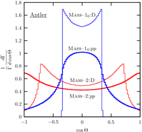
Figure 17: Comparison of the $\cos\Theta$ distribution in the $D$ rest frame (thin curves) and in the $pp$ lab frame with $\sqrt{s}=14\ {\,{\rm TeV}}$ (thick curves). The mass parameters used here are Mass-1₀ and Mass-2 defined in Tables 2 and 3.

At hadron colliders, the longitudinal motion of the particle $D$ is not determined even when $D$ is singly produced. Among the discussed kinematic variable, only the $\cos{\Theta}$ is affected, which is defined with a momentum in the $D$ rest frame. In order to see the longitudinal boost effects, we convert the $\cos{\Theta}$ distribution in the $D$ rest frame into that in the $pp$ frame at the LHC, by convoluting with the parton distribution functions of a proton. We have used CTEQ6 cteq6 . In Fig.17, we compare the normalized $\cos\Theta$ distribution in the $D$-rest frame (thin curves) with that in the $pp$ lab frame with $\sqrt{s}=14\ {\,{\rm TeV}}$ (thick curves). For simplicity we assume that the heavy particle $D$ is produced through the $s$-channel gluon fusion and/or $q\bar{q}$ annihilation.

In the massive visible particle case (mass-2), the cusped peaks vanish almost completely. In the massless case (mass-1₀), the pointed cusps become round, very hard to read. We conclude that the cusp in the $\cos{\Theta}$ distribution is not observeble at the LHC. In the $e^{+}e^{-}$ collisions, however, the fixed c.m. energy removes the longitudinal boost ambiguity, and thus the $\cos{\Theta}$ cusp provides valuable information on the missing particle mass.

V.3 Spin-correlation effect

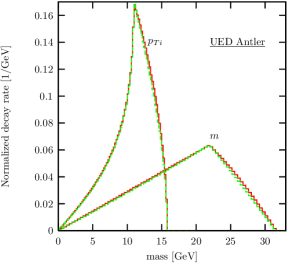
Figure 18: The invariant mass distribution $d{\Gamma}/dm$ and the individual transverse momentum distribution $d{\Gamma}/dp_{Ti}$ with and without spin correlations of ${Z^{(2)}}\to{L^{(1)}}{L^{(1)}}\to\ell^{-}B^{(1)}\ell^{+}B^{(1)}$ in the minimal UED model. We have set $1/R=500{\,{\rm GeV}}$ and ${\Lambda}R=20$.

The effects of the spin-correlation by the full matrix elements are different from new physics process to process. In addition, if we consider the associated production of the particle $D$ in order to control the SM background, the spin correlation effects get intertwined with the additional $p_{T}$ and/or longitudinal boost effects. To maximize the discovery significance, it is desirable to develop an individual strategy for each process in Eqs.(1)–(4), which is beyond the scope of this paper.

Generically, the positions of cusps and endpoints are not affected by the spin correlation effects since they are determined purely by the constrained phase space, i.e., by the mass relations Kim:2009si . In order to see this feature, we consider the ${Z^{(2)}}$ decay in the framework of the minimal UED model (mUED) ued :

$${Z^{(2)}}\to{L^{(1)}}+{L^{(1)}}\to\ell^{-}B^{(1)}+\ell^{+}B^{(1)}.$$ (61)

In Fig. 18, we show the $m$ and $p_{Ti}$ distributions including the full matrix elements of the process in Eq. (61) at the LHC with $\sqrt{s}=14{\,{\rm TeV}}$. We have fixed $1/R=500{\,{\rm GeV}}$ and ${\Lambda}R=20$, which generates the KK masses of $m_{D}=1048{\,{\rm GeV}}$, $m_{B}=515{\,{\rm GeV}}$, $m_{a}=0$, and $m_{X}=500.9{\,{\rm GeV}}$. First finite width effects are negligible: very degenerate mass spectrum in the mUED model yields very small total decay width such that ${\Gamma}_{B}/m_{B}\sim 10^{-4}$. Second the longitudinal boost effects do not apply to $m$ and $p_{Ti}$. As shown in Fig. 18, the spin correlations hardly change the $m$ and $p_{Ti}$ distributions. The distributions with and without the spin correlation effects are almost identical.

Brief comments on the SM background and detector simulation effects are in order here. In Ref. cusp , we have shown that the cusp structure survives over the SM backgrounds and the detector simulations in a benchmark process of $pp\to Z^{\prime}\to\tilde{\ell}^{+}\tilde{\ell}^{-}\to\ell^{+}{\tilde{\chi}^{0}_{1}}\ell^{-}{\tilde{\chi}^{0}_{1}}$ in a supersymmetry model with an extra $U(1)$ gauge field. In addition the missing particle mass as well as the intermediate particle mass can be determined, even though the uncertainty is about 10%. It was demonstrated that the analytic expression for the invariant mass distribution is very helpful to reconstruct the mass parameters by best-fitting.

VI Summary and Conclusions

In this paper, we have considered the antler decay topology of a parity-even heavy particle into two missing particles ($X_{1}$ and $X_{2}$) and two visible particles ($a_{1}$ and $a_{2}$) via intermediate on-shell particles ($B_{1}$ and $B_{2}$). We studied the singularity structures in various kinematic distributions, especially non-smooth peaks called the cusps. We show that the distributions of the invariant mass $m$ of $a_{1}$ and $a_{2}$, the individual transverse momentum $p_{Ti}$, and the $\cos\Theta$ develop conspicuous cusp structures. We have provided the detailed derivations for the positions of the cusps as well as the endpoints in terms of the particle masses. The analytic functional forms of the invariant mass and $\cos\Theta$ distributions have been also given.

The cusp and endpoint structures of the antler decay have a few advantages: $(i)$ if the parent particle mass $m_{D}$ is known from other decay channels, they can be used to determine both the missing particle and intermediate particle masses; $(ii)$ the cusped peaks are more identifiable than endpoints and kinks due to higher statistics at the kinematical maxima; $(iii)$ the simple configuration of outgoing particles, two visible particles and two missing particles, avoids combinatoric complication, which is troublesome in many missing particle mass measurement methods; $(iv)$ the position of the cusp is independent of the $S$-matrix element such as the spin correlation effects, since it is purely determined by the phase space.

We point out that the $p_{Ti}$ cusp and endpoint have some desirable features for observation. The $p_{Ti}$ cusp tends to be sharp irrespective of mass parameter regions. It is complementary to the robust $m$ cusp, which is sharp only when the masses are nearly degenerate. The $p_{Ti}$ endpoint is always located at fast-dropping end, which is easier to read off. Finally, the cusp position for the massive visible particle case is uniquely determined by the involved masses, while the $m$ cusp has two-fold ambiguity.

It is noted that the cusp structures have some limitations for the missing particle mass determination, especially at the LHC. The sharp cusped peaks in the $\cos\Theta$ distribution are not readily observable at the LHC, due to the longitudinal boost of the produced $D$ particle. The effects of the finite width of the intermediate particle could affect the cusp and endpoint in the individual transverse momentum distribution. However, for generically weakly coupled theories beyond the SM, the new particles for the antler decay have relatively small decay widths, and thus the $p_{Ti}$ cusp is expected to be preserved. The cusp in the invariant mass distribution, which is the most robust observable at the LHC, is most pronounced for a degenerate mass spectrum.

In addition, the relations among different cusps and endpoints help to identify the antler decay topology. For example, the $m_{T}$ maximum is equal to the $m$ maximum. The cusp and endpoint of $p_{Ti}$ distribution are half of those of $m$ distribution in the massless visible particle case. One can use these facts for the consistency of the assumptions on the event topology. Similar intriguing relations exist for the massive visible particle case.

In conclusion, if a new physics model accommodates an antler decay, the measurement of kinematic cusps and endpoints can be helpful to determine the missing particle mass as well as the intermediate particle mass. The proposed processes in various new physics models are expected to have stable cusp and endpoint structures in the $m$, $m_{T}$, and $p_{Ti}$ distributions at the LHC.

Appendix A Kinematic distributions in the symmetric Antler decay

In this Appendix, we derive the kinematic distributions of the invariant mass and the $\cos\Theta$ for the symmetric antler decays $D\to B_{1}+B_{2}\to a_{1}X_{1}+a_{2}X_{2}$ where $m_{B_{1}}\!=\!m_{B_{2}}\!\equiv\!m_{B}$, $m_{a_{1}}\!=\!m_{a_{2}}\!\equiv\!m_{a}$ and $m_{X_{1}}\!=\!m_{X_{2}}\!\equiv\!m_{X}$. We first describe the four-body phase space and choose special internal phase variables. For each four-momentum, we specify the reference frame in the superscript. For example, $k_{1}^{(B_{1})}$ is the four-momentum of $a_{1}$ in the rest frame of $B_{1}$. Since we calculate physical quantities mostly in the $D$ rest frame, we omit the superscript for the $D$ rest frame for simplicity. Note that this is different from the notation in the main text where we omit the superscript for momenta in the lab frame.

A.1 Four-body phase space

We consider four body decays of

$$D(P)\to a_{1}(k_{1})+a_{2}(k_{2})+X_{1}(k_{3})+X_{2}(k_{4}).$$ (62)

The differential decay rate of the process is

$$d{\Gamma}=\frac{1}{2m_{D}}\overline{|{\mathcal{M}}|^{2}}\;d\Phi_{4}(P;k_{1},k_{2},k_{3},k_{4}),$$ (63)

where $\overline{|{\mathcal{M}}|^{2}}$ is the helicity amplitude squared, and $d\Phi_{4}$ is the element of four-body phase space, defined by PDG ; han:pheno :

$$d\Phi_{4}(P;k_{1},\dots,k_{4})=(2\pi)^{4}\delta^{4}\left(P-\sum_{i=1}^{4}k_{i}\right)\,\prod_{i=1}^{4}\frac{d^{3}\mathbf{k}_{i}}{(2\pi)^{3}2E_{i}}.$$ (64)

If the decay in Eq. (62) is through the antler decay, i.e., through $D\to B_{1}B_{2}$ followed by $B_{i}\to a_{i}X_{i}(i=1,2)$, the helicity amplitude squared $\overline{|{\mathcal{M}}|^{2}}$ has two propagator factors of $B_{1}$ and $B_{2}$. Using the narrow width approximation $\Gamma_{B}/m_{B}\ll 1$, the matrix element squared can be expressed in terms of two Dirac delta functions:

$$\overline{|{\mathcal{M}}|^{2}} \equiv\widehat{|{\mathcal{M}}|^{2}}\;\frac{1}{(p_{1}^{2}-m_{B}^{2})^{2}+m_{B}^{2}{\Gamma}_{B}^{2}}\;\frac{1}{(p_{2}^{2}-m_{B}^{2})^{2}+m_{B}^{2}{\Gamma}_{B}^{2}}$$ (65)

$$\stackrel{{\scriptstyle\Gamma_{B}\ll m_{B}}}{{\longrightarrow}}\widehat{|{\mathcal{M}}|^{2}}\ \left(\frac{\pi}{m_{B}{\Gamma}_{B}}\right)^{2}\ \delta(p_{1}^{2}-m_{B}^{2})\ \delta(p_{2}^{2}-m_{B}^{2}),$$

where $p_{1}=k_{1}+k_{3}$ and $p_{2}=k_{2}+k_{4}$ are the momentum of $B_{1}$ and $B_{2}$, respectively. In this limit, $\widehat{|{\mathcal{M}}|^{2}}$ does not develop any singular behavior and still remains as a smooth function containing spin correlation information.

After the integration using delta functions, the differential decay width is simplified to

$$d{\Gamma}=\frac{1}{2^{15}\pi^{4}m_{D}m_{B}^{2}{\Gamma}_{B}^{2}}\,\widehat{|{\mathcal{M}}|^{2}}\,{\lambda}^{1/2}_{B}\ {\lambda}_{a}\,d\cos\theta_{1}d\cos\theta_{2}d\phi,$$ (66)

where ${\lambda}_{B}={\lambda}\left(1,{m_{B}^{2}}/{m_{D}^{2}},{m_{B}^{2}}/{m_{D}^{2}}\right)$, ${\lambda}_{a}={\lambda}\left(1,{m_{a}^{2}}/{m_{B}^{2}},{m_{X}^{2}}/{m_{B}^{2}}\right)$, and the standard kinematic function is ${\lambda}(a,b,c)=a^{2}+b^{2}+c^{2}-2ab-2ac+2bc$. The polar angles of $\theta_{1}$ and $\theta_{2}$ and the azimuthal angle $\phi$ are defined in Fig. 3. For simplicity, we use short-hand notations of

$$v_{1}\equiv\cos\theta_{1},\quad v_{2}\equiv\cos\theta_{2},$$ (67)

and name $dv_{1}dv_{2}d\phi$ the normalized four-body phase space ${d\widehat{\Phi}_{4}}$ of the antler decay:

$${d\widehat{\Phi}_{4}}=dv_{1}dv_{2}d\phi.$$ (68)

A.2 Change of variables and the independence between angular variables

For a general two body decay of $a\to bc$:

$$a(p_{a})\to b(p_{b})+c(p_{c}),$$ (69)

the energy-momentum conservation in the rest frame of the parent particle $a$ leads to

$$m_{a} = E^{(a)}_{b}+E^{(a)}_{c},$$ (70)

$${}{\bf p}^{(a)}_{b} = -{\bf p}^{(a)}_{c}.$$

From the on-shell conditions of $p_{i}^{2}=m_{i}^{2}~{}(i=b,c)$, the energies and momenta of the particles $b$ and $c$ are simply expressed by the rapidities $\eta_{b}$ and $\eta_{c}$:

$$E^{(a)}_{b} = \frac{m_{a}^{2}+m_{b}^{2}-m_{c}^{2}}{2m_{a}}\equiv m_{b}\cosh\eta_{b},$$ (71)

$$E^{(a)}_{c} = \frac{m_{a}^{2}-m_{b}^{2}+m_{c}^{2}}{2m_{a}}\equiv m_{c}\cosh\eta_{c},$$ (72)

$$\left|{\bf p}^{(a)}_{b}\right| = \left|{\bf p}^{(a)}_{c}\right|=m_{b}\sinh\eta_{b}=m_{c}\sinh\eta_{c}.$$ (73)

For the symmetric antler decay, the same masses of $m_{B}\!\equiv\!m_{B_{1}}\!=\!m_{B_{2}}$ and $m_{a}\!\equiv\!m_{a_{1}}\!=\!m_{a_{2}}$ lead to two independent rapidities:

$$\cosh\eta_{B}=\frac{m_{D}}{2m_{B}},\quad\cosh\eta_{a}=\frac{m_{B}^{2}-m_{X}^{2}+m_{a}^{2}}{2m_{a}m_{B}}.$$ (74)

Now we present less intuitive but more convenient kinematic variables. First, we consider the rapidity of $a_{2}$ in the rest frame of $B_{1}$, not $B_{2}$, denoted by $\alpha\equiv\eta^{(B_{1})}_{a_{2}}$:

$$\cosh\alpha=\cosh 2\eta_{B}\,\cosh\eta_{a}-v_{2}\,\sinh 2\eta_{B}\,\sinh\eta_{a},$$ (75)

where $v_{2}$ is defined in Eq. (67). The second useful variable is $u$, the cosine of the angle $\theta_{a_{1}a_{2}}^{(B_{1})}$ between $a_{1}$ and $a_{2}$ in the rest frame of $B_{1}$:

$$u=\frac{\mathbf{k}_{1}^{(B_{1})}\cdot\mathbf{k}_{2}^{(B_{1})}}{\left|\mathbf{k}_{1}^{(B_{1})}\right|\left|\mathbf{k}_{2}^{(B_{1})}\right|}=\frac{\sqrt{1-v_{1}^{2}}\sqrt{1-v_{2}^{2}}\,\cos\phi+(\sinh 2\eta_{B}-v_{2}\,\cosh 2\eta_{B})\,v_{1}}{\cosh 2\eta_{B}-v_{2}\,\sinh 2\eta_{B}}.$$ (76)

For simplicity, we define

$$v^{\prime}_{2} = \cosh 2\eta_{B}-v_{2}\,\sinh 2\eta_{B},$$ (77)

$${}v^{\prime\prime}_{2} = \sinh 2\eta_{B}-v_{2}\,\cosh 2\eta_{B}.$$

Then the azimuthal angle $\phi$ is inversely obtained by

$$\cos\phi=\frac{uv_{2}^{\prime}-v_{1}v_{2}^{\prime\prime}}{\sqrt{1-v_{1}^{2}}\sqrt{1-v_{2}^{2}}}.$$ (78)

The advantage of this new angular variable $u$ is that $d^{2}{\widehat{\Phi}_{4}}/dudv_{2}=\pi$: $u$ and $v_{2}$ are independent variables contrary to the expectation from the functional dependence of $u$ on $v_{1}$ and $v_{2}$ in Eq. (76). In order to show this non-trivial result, we begin with $d^{3}{\widehat{\Phi}_{4}}/dv_{1}dv_{2}d\phi=1$ in Eq. (68). We change the variable $\phi$ into $u$ as

$${d\widehat{\Phi}_{4}}=dv_{1}dv_{2}d\phi = dv_{1}dv_{2}du\left|\frac{{\partial}\phi}{{\partial}u}\right|$$

$$= dv_{1}dv_{2}du\frac{v_{2}^{\prime}}{\sqrt{(1-v_{1}^{2})(1-v_{2}^{2})-(uv_{2}^{\prime}-v_{1}v_{2}^{\prime\prime})^{2}}}$$

$$\equiv dv_{1}dv_{2}du\frac{v_{2}^{\prime}}{\sqrt{f(u,v_{1},v_{2})}}.$$

Since the integrand $v^{\prime}_{2}/\sqrt{f(u,v_{1},v_{2})}$ is not separable into products, $u$, $v_{1}$ and $v_{2}$ are not independent with one another. If we integrate one of the three variables, however, we have the statistical independence of the remaining two variables. First $v_{1}$ and $v_{2}$ are independent variables by definition. In order to see the independence of $v_{2}$ and $u$, we integrate $v_{1}$ out for given $u$ and $v_{2}$. The integration limit of $v_{1}$ is matched with the roots of $f(u,v_{1},v_{2})=0$ for fixed $u$ and $v_{2}$. The result of the integration is a simple constant:

$$\int^{v_{1}^{(\rm max)}}_{v_{1}^{(\rm min)}}dv_{1}\frac{v^{\prime}_{2}}{\sqrt{\left(v_{1}-v_{1}^{(\rm min)}\right)\left(v_{1}^{(\rm max)}-v_{2}\right)(v^{\prime}_{2})^{2}}}=\pi.$$ (80)

Therefore ${d\widehat{\Phi}_{4}}/dudv_{2}=\pi$ is also flat: $u$ and $v_{2}$ are independent. Similarly, one can show the independence of $u$ and $v_{1}$ from the symmetry under the exchange of $v_{1}$ and $v_{2}$.

A.3 The invariant mass distribution

The invariant mass $m$ of $a_{1}$ and $a_{2}$ is more simply expressed in terms of $\alpha$ and $u$ by

$$m^{2}=2m_{a}^{2}+2m_{a}^{2}(\cosh\eta_{a}\cosh\alpha-u\sinh\eta_{a}\sinh\alpha),$$ (81)

where $\alpha$ and $u$ are defined in Eqs. (75) and (76) respectively. The expression in the parenthesis of Eq. (81) is nothing but the cosine hyperbolic of the rapidity of the particle $a_{1}$ in the rest frame of $a_{2}$:

$$\chi \equiv \cosh\eta^{(a_{1})}_{a_{2}}=\frac{m^{2}}{2m_{a}^{2}}-1=\cosh\eta_{a}\cosh\alpha-u\sinh\eta_{a}\sinh\alpha.$$ (82)

Now let us change variables from $(u,v_{2})$ to $(\chi,\alpha)$:

$$dudv_{2}=d\chi d\alpha\frac{1}{\sinh 2\eta_{B}\sinh^{2}\eta_{a}}.$$ (83)

Note that the Jacobian factor is simply a constant. From $d^{2}{\widehat{\Phi}_{4}}/dudv_{2}=\pi$, we have

$$\frac{{d\widehat{\Phi}_{4}}}{d\chi}=\frac{\pi}{\sinh 2\eta_{B}\sinh^{2}\eta_{a}}\int^{\alpha_{\rm max}(\chi)}_{\alpha_{\rm min}(\chi)}d\alpha,$$ (84)

where $\alpha_{\rm min}(\chi)$ and $\alpha_{\rm max}(\chi)$ are the minimum and maximum of $\alpha$ variable at a given $\chi$, respectively.

In order to obtain ${\alpha}_{\min}(\chi)$ and ${\alpha}_{\max}(\chi)$, we use the conditions of $u\in[-1,1]$ and $v_{2}\in[-1,1]$. Then the definitions of $\cosh\alpha$ and $\chi$ in Eqs. (75) and (82), respectively, constrain the values of $\cosh\alpha$ and $\chi$ as

$$\cosh(2\eta_{B}-{\eta_{a}})\leq\cosh\alpha\leq\cosh(2\eta_{B}+{\eta_{a}}),$$ (85)

$$\cosh({\alpha}-{\eta_{a}})\leq\chi\leq\cosh({\alpha}+{\eta_{a}}).$$ (86)

Therefore, the values of $\alpha_{\rm min}(\chi)$ and $\alpha_{\rm max}(\chi)$ in Eq. (84) depend on the relative size between $\eta_{B}$ and $\eta_{a}/2$ or $\eta_{B}$ and $\eta_{a}$. This is related with the three different mass parameter regions of ${\mathcal{R}}_{1}$, ${\mathcal{R}}_{2}$, and ${\mathcal{R}}_{3}$ in Sec. III.1:

$${\mathcal{R}}_{1}:\eta_{B}<\frac{{\eta_{a}}}{2},\quad{\mathcal{R}}_{2}:\frac{{\eta_{a}}}{2}<\eta_{B}<{\eta_{a}},\quad\mathcal{R}_{3}:{\eta_{a}}<\eta_{B}.$$ (87)

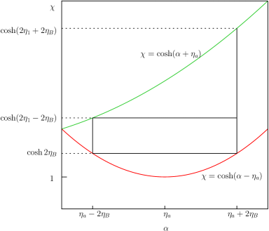
Figure 19: Allowed parameter space of $(\alpha,\chi)$ plane for the region ${\mathcal{R}}_{1}$.

Let us elaborate the derivation of ${\alpha}_{\min}(\chi)$ and ${\alpha}_{\max}(\chi)$ for the region ${\mathcal{R}}_{1}$. Figure 19 illustrates two curves of $\chi=\cosh(\alpha-\eta_{a})$ and $\chi=\cosh(\alpha+\eta_{a})$ in the parameter space of $(\alpha,\chi)$. Within the bound of $\eta_{a}-2\eta_{B}<\alpha<\eta_{a}+2\eta_{B}$ as in Eq.(85), ${\alpha}_{\min}(\chi)$ and ${\alpha}_{\max}(\chi)$ are different according to the value of $\chi$, summarized by

$$\begin{array}[]{c|cc|c}\hbox{ For }{\mathcal{R}}_{1}&~{}~{}~{}~{}~{}~{}{\alpha}_{\min}(\chi){}{}{}{}{}{}&~{}~{}~{}~{}~{}~{}{\alpha}_{\max}(\chi){}{}{}{}{}{}&\int d{\alpha}\\ \hline\cr 1<\chi<c_{2\eta_{B}}&{\eta_{a}}-\cosh^{-1}\chi&{\eta_{a}}+\cosh^{-1}\chi&2\cosh^{-1}\chi\\ c_{2\eta_{B}}<\chi<c_{2\eta_{a}-2{\eta_{B}}}&{\eta_{a}}-2\eta_{B}&{\eta_{a}}+2\eta_{B}&4\eta_{B}\\ c_{2\eta_{a}-2{\eta_{B}}}<\chi<c_{2\eta_{B}+2{\eta_{a}}}&-{\eta_{a}}+\cosh^{-1}\chi&{\eta_{a}}+2\eta_{B}&2\eta_{B}+2{\eta_{a}}-\cosh^{-1}\chi\end{array}$$ (92)

Here we use the simplified notation of $c_{x}\equiv\cosh x$. The derivations for ${\mathcal{R}}_{2}$ and ${\mathcal{R}}_{3}$ are similar and straightforward.

With the help of Eq. (84), the final expressions for $d{\widehat{\Phi}_{4}}/dm$ is given by

$$\left.\frac{1}{N}\frac{{d\widehat{\Phi}_{4}}}{dm}\right|_{{\mathcal{R}}_{1}} = \left\{\begin{array}[]{ll}2m\cosh^{-1}\left(\frac{m^{2}}{2m_{a}^{2}}-1\right),&\hbox{ if }1<\chi<c_{2\eta_{B}};\\ 4\eta_{B}m,&\hbox{ if }c_{2\eta_{B}}<\chi<c_{2({\eta_{a}}-\eta_{B})};\\ 2(\eta_{a}+\eta_{B})m-m\cosh^{-1}\left(\frac{m^{2}}{2m_{a}^{2}}-1\right),&\hbox{ if }c_{2({\eta_{a}}-\eta_{B})}<\chi<c_{2({\eta_{a}}+\eta_{B})},\end{array}\right.$$ (96)

$$\!\!\!\!\left.\frac{1}{N}\frac{{d\widehat{\Phi}_{4}}}{dm}\right|_{{\mathcal{R}}_{2}} = \left\{\begin{array}[]{ll}2m\cosh^{-1}\left(\frac{m^{2}}{2m_{a}^{2}}-1\right),&\hbox{ if }1<\chi<c_{2(\eta_{a}-\eta_{B})};\\ 2(\eta_{a}-\eta_{B})m+m\cosh^{-1}\left(\frac{m^{2}}{2m_{a}^{2}}-1\right),&\hbox{ if }c_{2({\eta_{a}}-\eta_{B})}<\chi<c_{2\eta_{B}};\\ 2(\eta_{a}+\eta_{B})m-m\cosh^{-1}\left(\frac{m^{2}}{2m_{a}^{2}}-1\right),&\hbox{ if }c_{2\eta_{B}}<\chi<c_{2({\eta_{a}}+\eta_{B})},\end{array}\right.$$ (100)

$$\left.\frac{1}{N}\frac{{d\widehat{\Phi}_{4}}}{dm}\right|_{{\mathcal{R}}_{3}} = \left\{\begin{array}[]{ll}2(\eta_{a}-\eta_{B})m+m\cosh^{-1}\left(\frac{m^{2}}{2m_{a}^{2}}-1\right),&\hbox{ if }c_{2({\eta_{a}}-\eta_{B})}<\chi<c_{2\eta_{B}};\\ 2(\eta_{a}+\eta_{B})m-m\cosh^{-1}\left(\frac{m^{2}}{2m_{a}^{2}}-1\right),&\hbox{ if }c_{2\eta_{B}}<\chi<c_{2({\eta_{a}}+\eta_{B})},\end{array}\right.$$ (103)

where the normalization factor $N$ is

$$N=\frac{\pi}{\sinh{2\eta_{B}}}\frac{1}{(m_{a}\sinh\eta_{a})^{2}}.$$ (104)

A.4 The angular distribution $d\Gamma/d\cos\Theta$

In this subsection, we derive ${d\widehat{\Phi}_{4}}/d\cos{\Theta}$, restricting ourselves to the massless visible particle case ($m_{a_{1}}\!=\!m_{a_{2}}\!=\!0$). Recall that $\Theta$ is the angle of a visible particle, say $a_{1}$, in the c.m. frame of $a_{1}$ and $a_{2}$, with respect to their c.m. moving direction in the $D$ rest frame. For ${d\widehat{\Phi}_{4}}/d\cos{\Theta}$, we begin with $d^{3}\widehat{\Phi}_{4}/dv_{1}dv_{2}d\phi=1$. The key point is the Jacobian factor from $dv_{1}dv_{2}d\phi$ to $d\cos{\Theta}$. For this goal, we first obtain the analytic expression of $\phi$ in terms of $v_{1}$, $v_{2}$, and $\cos{\Theta}$.

In the case of $m_{a}=0$, the $k_{1}$ and $k_{2}$ four-momenta in the $B_{1}$ rest frame become

$$k_{1}^{(B_{1})} = E^{(B_{1})}_{1}(1,\sqrt{1-v_{1}^{2}},0,-v_{1})=E_{\ell}(1,\hat{\mathbf{k}}_{1}),$$ (105)

$${}k_{2}^{(B_{1})} = E^{(B_{1})}_{1}(v_{2}^{\prime},\sqrt{1-v_{2}^{2}}\cos\phi,\sqrt{1-v_{2}^{2}}\sin\phi,-v_{2}^{\prime\prime})=E_{\ell}v_{2}^{\prime}(1,\hat{\mathbf{k}}_{2}),$$

where $E_{\ell}=m_{B}(1-m_{X}^{2}/m_{B}^{2})/2$, $\hat{\mathbf{k}}_{i}=\mathbf{k}_{i}/|\mathbf{k}_{i}|(i=1,2)$, and the definitions of $v_{2}^{\prime}$ and $v_{2}^{\prime\prime}$ are in Eq. (77). Defining $k\equiv k_{1}+k_{2}=(E_{\rm cm},\mathbf{k})$, we have some useful expressions of

$$m^{2} = 2E_{\ell}^{2}v_{2}^{\prime}(1-u),$$ (106)

$${}E_{\rm cm}^{(B_{1})} = E_{\ell}(1+v_{2}^{\prime}),$$

$${}|\vec{k}^{(B_{1})}|^{2} = E_{\ell}^{2}\{1+2v_{2}^{\prime}u+(v_{2}^{\prime})^{2}\}.$$

Now the Lorentz transformation matrix from the $B_{1}$ rest frame to the c.m. frame of $a_{1}a_{2}$ is

$${\Lambda}^{(a_{1}a_{2}\leftarrow B_{1})}=\left(\begin{array}[]{cc}{\gamma}_{\rm cm}&-\dfrac{\mathbf{k}^{(B_{1})\,T}}{m}\\[11.38092pt] -\dfrac{\mathbf{k}^{(B_{1})}}{m}&~{}~{}~{}~{}~{}I_{3\times 3}+\left({\gamma}_{\rm cm}-1\right)\hat{\mathbf{k}}^{(B_{1})}\hat{\mathbf{k}}^{(B_{1})\,T}\\ \end{array}\right),$$ (109)

where ${\gamma}_{\rm cm}={E_{\rm cm}^{(B_{1})}}/{m}$, and the superscript $T$ denotes the transpose of the vector. The three-momentum of $a_{1}$ particle in the c.m. frame of $a_{1}$ and $a_{2}$ is

$$\mathbf{k}_{1}^{(\rm cm)}=\left\{-\frac{E_{\rm cm}^{(B_{1})}}{m}\mathbf{k}^{(B_{1})}+\mathbf{k}_{1}+\left({\gamma}_{\rm cm}-1\right)(\hat{\mathbf{k}}^{(B_{1})}\cdot\mathbf{k}_{1}^{(B_{1})})\hat{\mathbf{k}}^{(B_{1})}\right\}.$$ (110)

Since $k$ in the $D$ rest frame is $k^{(D)}=-P_{D}^{(\rm cm)}=-{\Lambda}^{(a_{1}a_{2}\leftarrow B_{1})}P_{D}^{(B_{1})}$, we have

$$\mathbf{k}^{(D)}=-\left\{-\frac{E_{D}^{(B_{1})}}{m}\mathbf{k}+\mathbf{P}_{D}^{(B_{1})}+\left({\gamma}_{\rm cm}-1\right)(\hat{\mathbf{k}}^{(B_{1})}\cdot\mathbf{P}_{D}^{(B_{1})})\hat{\mathbf{k}}^{(B_{1})}\right\}.$$ (111)

The dot-product of $\mathbf{k}_{1}^{(\rm cm)}$ and $\mathbf{k}^{(D)}$ leads to $\cos{\Theta}$:

$$\cos\Theta=\frac{\mathbf{k}_{1}^{(\rm cm)}\cdot\mathbf{k}^{(D)}}{|\mathbf{k}_{1}^{(\rm cm)}||\mathbf{k}^{(D)}|}\,.$$ (112)

Finally we express $\cos{\Theta}$ in terms of $(v_{1},v_{2},\phi)$:

$$\cos{\Theta} = \frac{(v_{2}-v_{1})\,s_{\eta_{B}}}{\sqrt{2-\frac{1}{2}(v_{1}+v_{2})^{2}+\frac{1}{2}(v_{1}-v_{2})^{2}\,c_{2\eta_{B}}+2\sqrt{(1-v_{1}^{2})(1-v_{2}^{2})}\,\cos\phi}}.$$ (113)

Note that the maximum of $\cos{\Theta}$ occurs when $v_{1}=\pm 1$ and $v_{2}=\mp 1$, i.e., when the visible particles $a_{1}$ and $a_{2}$ are moving in the same direction. The maximum of $\cos{\Theta}$ in the $D$-rest frame is then

$$\left|\cos{\Theta}\right|_{\rm max}=\tanh\eta_{B}.$$ (114)

Finally $\cos\phi$ is expressed in terms of $v_{1}$, $v_{2}$, and $\Theta$:

$$\cos\phi=\dfrac{-1+\frac{1}{4}(v_{1}+v_{2})^{2}+\frac{1}{4}\left(\frac{2s_{\eta_{B}}^{2}}{\cos^{2}{\Theta}}-c_{2\eta_{B}}\right)(v_{1}-v_{2})^{2}}{\sqrt{(1-v_{1}^{2})(1-v_{2}^{2})}}\,,$$ (115)

where $s_{\eta}\equiv\sinh\eta$ for simplicity. For the Jacobian factor, we introduce three independent variables, $v_{+}$, $v_{-}$, and $t$, defined by

$$v_{\pm}=v_{1}\pm v_{2},\quad t=\frac{2s_{\eta_{B}}^{2}}{\cos^{2}{\Theta}}-c_{2\eta_{B}}.$$ (116)

Note that the maximum of $|\cos{\Theta}|$ in Eq.(114) leads to the $t$ integration range as $1\leq t<\infty$. Since

$${d\widehat{\Phi}_{4}}=dv_{1}dv_{2}d\phi=\frac{1}{2}dv_{+}dv_{-}dt\left|\frac{{\partial}\phi}{{\partial}t}\right|,$$ (117)

the differential four-body phase space with respect to $t$ is

$$\frac{{d\widehat{\Phi}_{4}}}{dt}=\frac{1}{4}\int dv_{+}dv_{-}^{2}\frac{1}{\sqrt{v_{-}^{2}(1-t^{2})+8t-2v_{+}^{2}t-8-2v_{+}^{2}}}.$$ (118)

The integration range is

$$0\leq v_{-}^{2}\leq\frac{-8-2v_{+}^{2}+8t-2v_{+}^{2}t}{t^{2}-1},$$ (119)

$$0\leq v_{+}^{2}\leq\frac{4(t-1)}{t+1}.$$ (120)

Finally the integration over $v_{-}$ and $v_{+}$ yields

$$\frac{{d\widehat{\Phi}_{4}}}{d\cos{\Theta}}=4\sqrt{2}\pi\sinh^{2}\eta_{B}\frac{1}{\sin^{3}{\Theta}}.$$ (121)

Appendix B The invariant mass distribution of generic antler decays

In this section, we present the analytic expression of the invariant mass distribution of generic non-symmetric antler decays with $m_{B_{1}}\!\neq\!m_{B_{2}}$, $m_{a_{1}}\!\neq\!m_{a_{2}}$ and $m_{X_{1}}\!\neq\!m_{X_{2}}$. The derivation is very similar to Appendix A, but in this general case the mass parameter space is divided into finer twelve regions. Since the derivation of the formulae for each region is long and tedious, we show only the results here.

B.1 Massive visible particles ($m_{a}\neq 0$)

In generic antler decays, there are in general six different rapidity parameters, given by

$$\cosh\eta_{X_{1}} = \frac{m_{B_{1}}^{2}+m_{X_{1}}^{2}-m_{a_{1}}^{2}}{2m_{X_{1}}m_{B_{1}}},\qquad\cosh\eta_{X_{2}}=\frac{m_{B_{2}}^{2}+m_{X_{2}}^{2}-m_{a_{2}}^{2}}{2m_{X_{2}}m_{B_{2}}},$$

$$\cosh\eta_{B_{1}} = \frac{m_{D}^{2}+m_{B_{1}}^{2}-m_{B_{2}}^{2}}{2m_{B_{1}}m_{D}},\qquad\cosh\eta_{B_{2}}=\frac{m_{D}^{2}+m_{B_{2}}^{2}-m_{B_{1}}^{2}}{2m_{B_{2}}m_{D}},$$

$$\cosh\eta_{a_{1}} = \frac{m_{B_{1}}^{2}+m_{a_{1}}^{2}-m_{X_{1}}^{2}}{2m_{a_{1}}m_{B_{1}}},\qquad\cosh\eta_{a_{2}}=\frac{m_{B_{2}}^{2}+m_{a_{2}}^{2}-m_{X_{2}}^{2}}{2m_{a_{2}}m_{B_{2}}}.$$ (122)

We define

$$\eta_{++} = \eta_{B_{1}}+\eta_{B_{2}}+\eta_{a_{1}}+\eta_{a_{2}},$$ (123)

$$\eta_{+-} = |\eta_{B_{1}}+\eta_{B_{2}}+\eta_{a_{1}}-\eta_{a_{2}}|,$$ (124)

$$\eta_{-+} = |\eta_{B_{1}}+\eta_{B_{2}}-\eta_{a_{1}}+\eta_{a_{2}}|,$$ (125)

$$\eta_{--} = |\eta_{B_{1}}+\eta_{B_{1}}-\eta_{a_{1}}-\eta_{a_{2}}|.$$ (126)

From positive definite definition of the rapidity, $\eta_{++}$ is the larges among four $\eta_{\pm\pm}$’s. However the relative size of the other three $\eta$’s is different according to the mass parameters. We order $\eta_{+-}$, $\eta_{-+}$ and $\eta_{--}$ and name them to be $\eta_{1}\leq\eta_{2}\leq\eta_{3}$. We have 6 regions depending on this ordering:

$$\eta_{+-}\leq\eta_{-+}\leq\eta_{--},\qquad\eta_{-+}\leq\eta_{+-}\leq\eta_{--},$$

$$\eta_{+-}\leq\eta_{--}\leq\eta_{-+},\qquad\eta_{-+}\leq\eta_{--}\leq\eta_{+-},$$

$$\eta_{--}\leq\eta_{+-}\leq\eta_{-+},\qquad\eta_{--}\leq\eta_{-+}\leq\eta_{+-}.$$

To obtain $d{\Gamma}/dm$, we introduce the general $\chi$, defined by

$$\chi\equiv\cosh\eta_{a_{2}}^{(a_{1})}=\frac{m^{2}-m_{a_{1}}^{2}-m_{a_{2}}^{2}}{2m_{a_{1}}m_{a_{2}}}.$$ (127)

The general invariant mass distribution have 12 different cases in total, given by

• If $|\eta_{B_{1}}+\eta_{B_{2}}-\eta_{a_{2}}|\geq\eta_{a_{1}}$ or $\eta_{B_{1}}+\eta_{B_{2}}+\eta_{a_{2}}\leq\eta_{a_{1}}$,

  $$\frac{1}{\tilde{N}}\frac{{d\widehat{\Phi}_{4}}}{dm}=\begin{cases}\begin{array}[]{ll}-\eta_{1}m+m\cosh^{-1}\left(\frac{m^{2}-m_{a_{1}}^{2}-m_{a_{2}}^{2}}{2m_{a_{1}}m_{a_{2}}}\right),&\mbox{ if $c_{\eta_{1}}\leq\chi\leq c_{\eta_{2}}$, }\\ \eta_{2}-\eta_{1},&\mbox{ if $c_{\eta_{2}}\leq\chi\leq c_{\eta_{3}}$, }\\ \eta_{++}-\cosh^{-1}\left(\frac{m^{2}-m_{a_{1}}^{2}-m_{a_{2}}^{2}}{2m_{a_{1}}m_{a_{2}}}\right),&\mbox{ if $c_{\eta_{3}}\leq\chi\leq c_{\eta_{++}}$, }\\ 0,&\mbox{ otherwise.}\end{array}\end{cases}$$ (128)

• If $|\eta_{B_{1}}+\eta_{B_{2}}-\eta_{a_{2}}|<\eta_{a_{1}}<\eta_{B_{1}}+\eta_{B_{2}}+\eta_{a_{2}}$,

  $$\frac{1}{\tilde{N}}\frac{{d\widehat{\Phi}_{4}}}{dm}=\begin{cases}\begin{array}[]{ll}2m\cosh^{-1}\left(\frac{m^{2}-m_{a_{1}}^{2}-m_{a_{2}}^{2}}{2m_{a_{1}}m_{a_{2}}}\right),&\mbox{ if $1\leq\chi\leq c_{\eta_{1}}$, }\\ -\eta_{1}m+m\cosh^{-1}\left(\frac{m^{2}-m_{a_{1}}^{2}-m_{a_{2}}^{2}}{2m_{a_{1}}m_{a_{2}}}\right),&\mbox{ if $c_{\eta_{1}}\leq\chi\leq c_{\eta_{2}}$, }\\ (\eta_{1}+\eta_{2})m,&\mbox{ if $c_{\eta_{2}}\leq\chi\leq c_{\eta_{3}}$, }\\ \eta_{++}m-m\cosh^{-1}\left(\frac{m^{2}-m_{a_{1}}^{2}-m_{a_{2}}^{2}}{2m_{a_{1}}m_{a_{2}}}\right),&\mbox{ if $c_{\eta_{3}}\leq\chi\leq c_{\eta_{++}}$, }\\ 0,&\mbox{ otherwise.}\end{array}\end{cases}$$ (129)

Here the normalization factor $\tilde{N}$ is given by

$$\tilde{N}=\frac{\pi}{m_{a_{1}}m_{a_{2}}\sinh 2\eta_{B}\sinh\eta_{a_{1}}\sinh\eta_{a_{2}}}.$$ (130)

Note that the minimum of the invariant mass distribution can be different from $m_{a_{1}}+m_{a_{2}}$, according to the mass parameter regions. Crucial is whether the kinematic configuration that $a_{1}$ and $a_{2}$ are relatively at rest is allowed.

B.2 Massless visible particles ($m_{a}=0$)

In this subsection, we present the invariant mass distribution for massless visible particle but different intermediate particle cases, i.e., when $m_{B_{1}}\neq m_{B_{2}}$ and $m_{a_{1}}=m_{a_{2}}=0$. In this case, $\eta_{--}$ is always larger than $\eta_{+-}$ and $\eta_{-+}$, leading to $\eta_{3}=\eta_{--}$. Here we need to consider only the leading terms of ${\mathcal{O}}\left(m_{a_{1}}^{-1}m_{a_{2}}^{-1}\right)$, which are absent in $\cosh\eta_{+-}$ and $\cosh\eta_{-+}$. Therefore, the invariant mass distribution is divided into three regions. Using $\cosh^{-1}x=\ln(x+\sqrt{x^{2}-1})\approx\ln(2x)$ for $x\gg 1$, we have

$$\frac{{d\widehat{\Phi}_{4}}}{dm}\propto\begin{cases}\begin{array}[]{ll}m\log\left(\frac{m_{\rm max}^{(0)}}{m_{\rm cusp}^{(0)}}\right),&\mbox{ if $0<m<m_{\rm cusp}^{(0)}$ ; }\\ m\log\left(\frac{m_{\rm max}^{(0)}}{m}\right),&\mbox{ if $m_{\rm cusp}^{(0)}<m<m_{\rm max}^{(0)}$;}\\ 0,&\mbox{ otherwise, }\end{array}\end{cases}$$ (131)

where

$$m_{\rm cusp}^{(0)} = \sqrt{\left(\frac{m_{B_{1}}^{2}-m_{X_{1}}^{2}}{m_{B_{1}}}\right)\left(\frac{m_{B_{2}}^{2}-m_{X_{2}}^{2}}{m_{B_{2}}}\right)}\,\exp\left(-\frac{\eta_{B_{1}}+\eta_{B_{2}}}{2}\right),$$ (132)

$$m_{\rm max}^{(0)} = \sqrt{\left(\frac{m_{B_{1}}^{2}-m_{X_{1}}^{2}}{m_{B_{1}}}\right)\left(\frac{m_{B_{2}}^{2}-m_{X_{2}}^{2}}{m_{B_{2}}}\right)}\,\exp\left(\frac{\eta_{B_{1}}+\eta_{B_{2}}}{2}\right).$$ (133)

This is the generalized results of Eqs. (50) and (51). Note that the product $m_{\rm cusp}^{(0)}m_{\rm max}^{(0)}$ depends only on the second step decays of $B_{1}\rightarrow X_{1}a_{1}$ and $B_{2}\rightarrow X_{2}a_{2}$ while the ratio $m_{\rm max}^{(0)}/m_{\rm cusp}^{(0)}$ only on the first step decay of $D\rightarrow B_{1}B_{2}$.

References

- (1) E. Komatsu et al. [WMAP Collaboration], Astrophys. J. Suppl. 180, 330 (2009).
- (2) G. Bertone, D. Hooper and J. Silk, Phys. Rept. 405, 279 (2005).
- (3) G. Jungman, M. Kamionkowski and K. Griest, Phys. Rept. 267, 195 (1996); M. Battaglia, A. De Roeck, J. R. Ellis, F. Gianotti, K. A. Olive and L. Pape, Eur. Phys. J. C 33, 273 (2004).
- (4) G. Servant and T. M. P. Tait, Nucl. Phys. B 650, 391 (2003); F. Burnell and G. D. Kribs, Phys. Rev. D 73, 015001 (2006); K. Kong and K. T. Matchev, JHEP 0601, 038 (2006).
- (5) I. Low, JHEP 0410, 067 (2004); A. Birkedal, A. Noble, M. Perelstein and A. Spray, Phys. Rev. D 74, 035002 (2006); J. Hubisz and P. Meade, Phys. Rev. D 71, 035016 (2005).
- (6) For a review, see e.g. , H. Baer and X. Tata, “Dark matter and the LHC,” arXiv:0805.1905 [hep-ph].
- (7) H. C. Cheng, J. F. Gunion, Z. Han, G. Marandella and B. McElrath, JHEP 0712, 076 (2007).
- (8) ALTAS Collaboration, Expected Performance of the ATLAS Experiment: Detector, Trigger and Physics, CERN-OPEN-2008-020; CMS Collaboration, Physics Technical Design Report, Volume 2, CERN/LHCC 2006-021.
- (9) M. Burns, K. Kong, K. T. Matchev and M. Park, JHEP 0903, 143 (2009).
- (10) I. Hinchliffe, F. E. Paige, M. D. Shapiro, J. Soderqvist and W. Yao, Phys. Rev. D 55, 5520 (1997); H. Bachacou, I. Hinchliffe and F. E. Paige, Phys. Rev. D 62, 015009 (2000); B. C. Allanach, C. G. Lester, M. A. Parker and B. R. Webber, JHEP 0009, 004 (2000); B. K. Gjelsten, D. J. . Miller and P. Osland, JHEP 0412, 003 (2004); B. K. Gjelsten, D. J. . Miller and P. Osland, JHEP 0506, 015 (2005).
- (11) M. M. Nojiri, G. Polesello and D. R. Tovey, arXiv:hep-ph/0312317; K. Kawagoe, M. M. Nojiri and G. Polesello, Phys. Rev. D 71, 035008 (2005).
- (12) H. C. Cheng, D. Engelhardt, J. F. Gunion, Z. Han and B. McElrath, Phys. Rev. Lett. 100, 252001 (2008); H. C. Cheng, J. F. Gunion, Z. Han, G. Marandella and B. McElrath, JHEP 0712, 076 (2007).
- (13) C. G. Lester and D. J. Summers, Phys. Lett. B 463, 99 (1999).
- (14) A. Barr, C. Lester and P. Stephens, J. Phys. G 29, 2343 (2003); M. M. Nojiri and M. Takeuchi, JHEP 0810, 025 (2008); P. Meade and M. Reece, Phys. Rev. D 74, 015010 (2006); S. Matsumoto, M. M. Nojiri and D. Nomura, Phys. Rev. D 75, 055006 (2007); C. Lester and A. Barr, JHEP 0712, 102 (2007).
- (15) W. S. Cho, K. Choi, Y. G. Kim and C. B. Park, Phys. Rev. Lett. 100, 171801 (2008); B. Gripaios, JHEP 0802, 053 (2008); A. J. Barr, B. Gripaios and C. G. Lester, JHEP 0802, 014 (2008); W. S. Cho, K. Choi, Y. G. Kim and C. B. Park, JHEP 0802, 035 (2008); M. M. Nojiri, Y. Shimizu, S. Okada and K. Kawagoe, JHEP 0806, 035 (2008).
- (16) M. Serna, JHEP 0806, 004 (2008); M. M. Nojiri, K. Sakurai, Y. Shimizu and M. Takeuchi, JHEP 0810, 100 (2008).
- (17) M. M. Nojiri, Y. Shimizu, S. Okada and K. Kawagoe, JHEP 0806, 035 (2008).
- (18) T. Han, I. W. Kim and J. Song, Phys. Lett. B 693, 575 (2010).
- (19) I. W. Kim, Phys. Rev. Lett. 104, 081601 (2010).
- (20) W. S. Cho, D. Kim, K. T. Matchev and M. Park, arXiv:1206.1546 [hep-ph].
- (21) T. Han, I. W. Kim and J. Song, arXiv:1206.5641 [hep-ph].
- (22) A. Djouadi, Phys. Rept. 459, 1 (2008).
- (23) M. Baumgart, T. Hartman, C. Kilic and L. T. Wang, JHEP 0711, 084 (2007); M. Cvetic and P. Langacker, arXiv:hep-ph/9707451.
- (24) A. Datta, K. Kong and K. T. Matchev, Phys. Rev. D 72, 096006 (2005) [Erratum-ibid. D 72, 119901 (2005)]; H. C. Cheng, J. L. Feng and K. T. Matchev, Phys. Rev. Lett. 89, 211301 (2002).
- (25) S. Kretzer, H. L. Lai, F. I. Olness, W. K. Tung, Phys. Rev. D69, 114005 (2004).
- (26) H. C. Cheng, K. T. Matchev and M. Schmaltz, Phys. Rev. D 66, 036005 (2002); T. Appelquist, H. C. Cheng and B. A. Dobrescu, Phys. Rev. D 64, 035002 (2001).
- (27) W. M. Yao et al. [Particle Data Group], J. Phys. G 33, 1 (2006).
- (28) T. Han, “Collider phenomenology: Basic knowledge and techniques,” hep-ph/0508097.