The inner equation for generalized standard maps

Abstract

We study particular solutions of the inner equation associated to the splitting of separatrices on generalized standard maps. An exponentially small complete expression for their difference is obtained. We also provide numerical evidence that the inner equation provides quantitative information of the splitting of separatrices even in the case when the limit flow does not.

1 Introduction

The phenomenon of the splitting of separatrices occurs when a dynamical system having an invariant object (a fixed point, a periodic orbit, a torus, etc.) with coincident branches of its stable and unstable invariant manifolds (a separatrix), is perturbed. Generically, a new invariant object of the perturbed system arises which still possesses stable and unstable invariant manifolds but which no longer coincide.

The problem of measuring the size of this splitting is long standing in Dynamics. It is related to the existence of transversal homoclinic points and, consequently, with the non-integrability and with the size of the stochastic zone of the system under study.

The most popular tool for measuring the splitting of separatrices is the Melnikov approach [Mel63]. It is based on classical perturbation theory and provides a first order approximation for the splitting by using the distance between the stable and unstable invariant manifolds of the perturbed system. Nevertheless there are plenty of interesting (and in some sense generic) situations where this approach fails: when the Melnikov function does not predict correctly the size of the splitting or when no Melnikov function is available, for instance, when integrable systems near simple resonances are perturbed. In this case, Poincaré already detected in [Poi99] that the separatrix splits but it turns out that the size of this splitting is exponentially small in the perturbation parameter, what it is usually known as a beyond-all-orders phenomenon. Consequently a direct application of a first order perturbation theory never will be able to provide a good estimation for this exponentially small splitting. There are other settings, related for instance to Arnold diffusion and fluid transport, when the splitting of separatrices is exponentially small in the perturbation parameter, but from now on we will restrict ourselves to the case of near identity, analytic, area-preserving maps.

1.1 Exponentially small splitting of separatrices in analytic maps

Throughout this introduction we will avoid precise statements and technicalities but we will give the main ideas about the exponentially small phenomenon.

Consider an area preserving analytic map, close to the identity, that is, a map which can be written as

$$G(z,h)=z+hg(z,h),\;\;\;\;z\in\mathbb{R}^{2}$$ (1)

where $h$ is a small parameter and $g(0,h)=0$, so that the origin is a fixed point for any value of $h$. Assume also that the origin is a weakly hyperbolic fixed point. Namely, redefining the parameter $h$ if necessary, the eigenvalues $\lambda,\lambda^{-1}$ of $DG(0)$ are of the form $\lambda=\text{e}^{h}=1+O(h)$. In this case, there exist $W^{{\rm s}}$ and $W^{{\rm u}}$, the stable and unstable invariant manifolds of the origin, respectively. The goal is to measure the discrepancy between these invariant manifolds. Notice that, since for $h=0$ the map $G(z,0)=z$, this is a beyond-all-orders phenomenon. The strategy is to not consider the first approximation of the map $G$ as simply taking $h=0$, but as the time $h$ map of the vector field

$$z^{\prime}=g(z,0).$$ (2)

It can be seen, for instance [FS90], that this approximation holds under generic and checkable assumptions. If the vector field (2) possesses a homoclinic connection $\gamma_{0}$ associated to the origin (the fixed point), then one expects that the exponentially small splitting of separatrices phenomenon arises for maps of the form (1). In fact in [FS90] is proved that, for any $p\in W^{{\rm s}}$

$$\text{dist}(p,W^{{\rm u}})\leq K_{\sigma}\text{e}^{-2\pi\sigma/h}$$ (3)

being $\sigma>0$ and $K_{\sigma}$ a constant depending on $\sigma$ and $p$, but independent of $h$. Nevertheless this upper bound is not useful for deciding whether the separatrix $\gamma_{0}$ splits or not. It turns out to be mandatory to obtain an expression for the asymptotic behavior of the splitting.

We emphasize here that, even when the distance between $W^{{\rm s}}$ and $W^{{\rm u}}$ seems a good choice for measuring the splitting, it depends on the point $p$. This is because this measure does not exploit the area preserving character of our map. There are several quantities more appropriate for this task. One of them is the Lazutkin invariant (see formula (11) in Section 2.1) which is related to the angle between both $W^{{\rm s}}$ and $W^{{\rm u}}$ at a homoclinic point. An upper bound similar to (3) for the Lazutkin invariant can be obtained but with $K_{\sigma}$ depending only on $\sigma$.

If the asymptotic behavior for the splitting has to be proved, the first question that arises from (3), is how much bigger $\sigma$ could be. To find this optimal value of $\sigma$ one has to know the analyticity domain of $\gamma_{0}$, the homoclinic connection of the vector field (2). It is proven in [Fon95] that $\gamma_{0}$ has complex singularities, henceforth it is analytic in a maximal complex strip $\{t\in\mathbb{C}:|\text{Im}t|<\sigma_{0}\}$. The bound (3) holds for any $\sigma<\sigma_{0}$, changing $K_{\sigma}$ appropriately. Notice that if we take any fixed $\sigma_{*}<\sigma_{0}$, we do not obtain a sharp upper bound, simply because the result also holds for $\sigma$, with $\sigma_{*}<\sigma<\sigma_{0}$ and henceforth, taking $h$ small enough we get a better estimate than the previous one. In consequence any asymptotic formula will require taking $\sigma$ arbitrarily close to $\sigma_{0}$ as a function of $h$.

The key point for proving the bound (3) is to obtain good parameterizations for the invariant manifolds $W^{{\rm s}}$, $W^{{\rm u}}$, which are analytic in the complex strip $\{t\in\mathbb{C}:|\text{Im}t|<\sigma\}$ with $\sigma<\sigma_{0}$. The natural parameterization for the invariant manifolds are functions $\gamma^{{\rm u},{\rm s}}(t)$ that satisfy

$$G(\gamma^{{\rm u},{\rm s}}(t),h)=\gamma^{{\rm u},{\rm s}}(t+h).$$ (4)

Notice that the homoclinic connection $\gamma_{0}$ satisfies this invariance equation for the time $h$ flow of the vector field (2). As we have mentioned in the above paragraph, to obtain an asymptotic formula for the splitting it is necessary to find solutions of the invariance equation (4) defined for values of $t$ arbitrarily close to $\sigma_{0}$ as a function of $h$. Since the strip is limited by the singularities of the homoclinic connection $\gamma_{0}$, this study becomes harder when the values of $t$ are closer to these singularities. The inner equation is a suitable approximation of the invariance equation (4) for values of $t$ close to these singularities.

The main goal of this paper is to derive the inner equation for a large set of area-preserving maps (the so called generalized standard maps) and to obtain information about some special solutions and their difference. This is a first step in the proof of an asymptotic formula for the splitting of the invariant manifolds for these maps, but obtaining this formula is beyond the scope of this work. Nevertheless we will provide some numerical results which, combined with heuristic arguments (see Section 4, in particular formula (46)) support the relation between the splitting and the inner equation.

1.2 The inner equation. An overview

The study of the inner equation has been at the heart of the proof of the exponentially small splitting of separatrices in many examples, for maps [Gel99, MSS11a, MSS11b] as well as for flows [GOS10].

In the case of area-preserving analytic maps, the use of the inner equation dates back to [Laz03], where a scheme to obtain an asymptotic formula for the splitting of separatrices of the Chirikov standard map was established. In that paper, a particular instance of the inner equation was introduced: the so called semi-standard map. Further development of the ideas in [Laz03] lead to the first rigorous proof of the asymptotic formula for the Chirikov standard map in [Gel99]. A brief discussion on the splitting size on the Chirikov standard map can be found in [Gel00b]. From the same authors, the survey on exponentially small phenomena [GL01] introduces, among other things, the inner equations associated to polynomial standard maps, and lists in an informal way asymptotic formulas for the splitting of separatrices in those cases. It is also remarkable that in the paper [GS01] resurgence theory is applied to the study of the solutions of the inner equation associated to the area preserving Hénon map. This paper is strongly related to [Gel00c]. Also in the study of perturbation of the McMillan map [MSS11a, MSS11b] resurgence methods were applied to study the inner equation. Summarizing, one can find rigorous results on the inner equation in [Gel99, GS01, MSS11b] in particular examples which are covered under our present work, which also includes and generalizes the ones present in [GL01] and the numerical study [GS08].

In the case of flows, the inner equation has been a successful tool to measure the splitting of separatrices when the Melnikov function fails to predict the size of the splitting, like in the rapidly forced pendulum (see [Gel00a, GOS10] or [BFGS11] for a generalization to arbitrary polynomial Hamiltonian systems of one and a half degrees of freedom, following the study on the inner equation in [Bal06]). A different technique based on continuous averaging to study the exponentially small behavior of the splitting can be found in [Tre97].

The purpose of the present paper is twofold, a combination of rigorous theoretical results in a general setting and numerical experiments avoiding lengthy proofs in particular examples. One of the numerical examples shows a a type of behavior that is not covered by the surveys [GL01, GS08] (see the end of this section).

We study some second order difference equations, called inner equations, which have the form either

$$\phi(z+1)-2\phi(z)+\phi(z-1)=-\phi^{n}(z)+G(\phi(z))$$

or

$$\phi(z+1)-2\phi(z)+\phi(z-1)=-\text{e}^{n\phi(z)}+G(\text{e}^{\phi(z)}),$$

depending on the class of maps under consideration, and where $G(w)$ is an analytic function such that $G(w)=\mathcal{O}(w^{n+1})$.

These equations appear, in particular, in the problem of exponentially small splitting of separatrices in generalized standard maps (see next Section for definitions), but they can appear in studies of other types of maps (with parabolic fixed points, for instance), and, with this applicability in mind, we consider them in their full generality (see equations (27) and (28)). In particular, our present results generalize those on the inner equations appearing in [Laz03, Gel99, Gel00b, GL01, GS01, MSS11a, MSS11b]. It is important to remark that in the previous literature on the subject the symmetries of the particular problems under consideration where exploited extensively in the proofs. Our present formulation does not rely on additional symmetries, making it suitable for applications. In particular, we provide all the technical details and complete proofs of the statements concerning the inner equations and their solutions. As a side comment for the specialists, there are several technical improvements in the proofs of our theoretical results, which we expect can be applied in other problems related to difference equations.

We describe a large set of formal solutions of these inner equations, from which some true solutions are obtained, and we derive a complete formula for their difference. The main results are collected in Section 3, while Section 2 plays the role of a more detailed introduction of the problem and description of some of the known results. Sections 5, 6 and 7 are devoted to prove the theoretical results, while Section 4 contains the numerical results with a non-rigorous exposition of their relation to the developed theory. It should be remarked that the relation between the inner equation and the actual computation of the splitting, in the particular cases where proofs are available (see [Gel99, MSS11a, MSS11b]), is lengthy and full of technicalities. Our exposition here tries to give the reader an idea of the link between the inner equation and splitting size, by making very strong assumptions, in order to explain the obtained numerical results. These assumptions are fully proved in the literature for the Chirikov standard map and the McMillan map.

The numerical experiments have been conducted to test the applicability of the theoretical results. Although academic in nature, they show the relation between the splitting of separatrices and the difference between two solutions of the inner equation. Moreover, the main example exhibits a behavior that is not covered by the surveys [GL01, GS08]. In this example, given by the map

$$\begin{pmatrix}x\\ y\end{pmatrix}\mapsto\begin{pmatrix}x+y+\varepsilon(x-x^{3})-\varepsilon^{2}x^{7}\\ y+\varepsilon(x-x^{3})-\varepsilon^{2}x^{7}\end{pmatrix},$$

where $\varepsilon$ is a small parameter, although the size of the splitting is much larger than the guess suggested by [FS90], the leading term of its asymptotic behavior is provided by the inner equation. As a matter of fact, the splitting size in this example behaves asymptotically when $\varepsilon\to 0$ as

$$\frac{A}{h^{10/3}}\text{exp}\left(-\frac{\pi^{2}}{h}+\frac{2^{5/4}\sqrt{\pi}\Gamma(3/4)^{2})}{h^{1/2}}\right)(1+\text{higher order terms}),$$

where $\varepsilon=4\sinh^{2}(h/2)$ and $A$ is a constant related to some inner equation, while the naïve guess provided by the limit flow (see Section 2 for details), in this case the Duffing equation $\ddot{x}=x-x^{3}$, would be exponential with exponent $-\pi^{2}/h$. That is, the correction term is larger than any power of $h$. See Sections 2.4 and 4.

We remark that although the computation of the actual splitting has been performed by using the multiple precision package PARI-GP, the computation of the leading term has been achieved by using the standard long double precision in C.

2 Generalized standard maps and exponentially small splitting of separatrices

2.1 Generalized standard maps

We will say that an area preserving map $(x^{*},y^{*})=F(x,y)$ is a generalized standard map if it can be written in the form

$$\left\{\begin{aligned} x^{*}&=x+y+f(x,h),\\ y^{*}&=y+f(x,h),\end{aligned}\right.$$ (5)

where $h$ is a small parameter. We will assume that $f$ depends analytically in its arguments in $|h|<h_{0}$, $|x|<\rho_{0}$, for some fixed $h_{0},\rho_{0}>0$. We will be interested in the case when the origin is a fixed point of $F$, that is, $f(0,h)=0$. Moreover, we will assume the origin to be weakly hyperbolic, although our study may be applied also to the case of a parabolic fixed point.

The parameter $h$ is chosen in such a way that $\text{spec}\,DF(0,0)=\{\text{e}^{h},\text{e}^{-h}\}$. This last condition is equivalent to impose $f^{\prime}(0,h)=\frac{\partial}{\partial x}f(0,h)=\varepsilon$, with $\varepsilon=4\sinh^{2}(h/2)$. We further assume that

$$f(x,h)=\sum_{k\geq 0}f_{k}(x)h^{k+2}=\varepsilon f_{0}(x)+O(h^{3}x).$$ (6)

Under these conditions, the map (5) can be written as a close to the identity map: with the scaling $\tilde{x}=x$, $h\tilde{y}=y$, it becomes (using again $x$ and $y$ as variables)

$$\left\{\begin{aligned} x^{*}&=x+hy+O(h^{2}x),\\ y^{*}&=y+hf_{0}(x)+O(h^{2}x).\end{aligned}\right.$$ (7)

When $h$ is small, the map (7) is well approximated by the time $h$ map of the flow of the Hamiltonian system

$$\left\{\begin{aligned} \dot{x}&=y,\\ \dot{y}&=f_{0}(x).\end{aligned}\right.$$ (8)

We assume that the origin in (8), which is a fixed point, possesses a homoclinic connection, $\gamma_{0}(t)=(x_{0}(t),y_{0}(t))$. By a shift on $t$, we can choose $\gamma_{0}$ such that $x_{0}$ is an even function, that is, $\gamma_{0}$ intersects transversally the line $\{y=0\}$ at $t=0$. The invariant manifolds of the origin for the map (7) are close to this homoclinic connection. Hence, if $h$ is small, by the conservation of the area, they must intersect. It is not difficult to check that the expansions in powers of $h$ of the stable and unstable curves coincide. As a consequence, the expansion of the angle of intersection in powers of $h$ vanishes, which, in view of the analytic nature of the problem, suggests that this angle may have an exponentially small behavior in $h$. In fact, Fontich and Simó, in [FS90], obtained an exponentially small upper bound for the angle. They showed that if $\gamma_{0}$ is analytic in the complex strip $\{|\text{Im}t|<\sigma_{0}\}$ and the map $F$ is defined around the homoclinic orbit, then, for any $0<\sigma<\sigma_{0}$, the distance between the stable and the unstable manifold of the origin of (7) is bounded by $K_{\sigma}\text{e}^{-2\pi\sigma/h}$, for any $0<h<h_{\sigma}$, where $K_{\sigma}$ and $h_{\sigma}$ are positive constants depending on $\sigma$ and $K_{\sigma}$ depends also on the point where this distance is measured. Restoring to the original variables, the same applies to the invariant manifolds of the origin of (5).

Equivalently, a natural parametrization $\gamma(t)=(x(t),y(t))$ of the invariant manifolds of the origin of (5), when condition (6) is satisfied, that is, a parametrization satisfying $F\circ\gamma(t)=\gamma(t+h)$, must be a solution of the difference equation

$$x(t+h)-2x(t)+x(t-h)=f(x(t),h),$$ (9)

with $y(t)=x(t)-x(t-h)$. This equation implies that the curve $\gamma=(x,y)$ is invariant by $F$ and the action of $F$ on $\gamma$ is conjugated to the shift on the parameter $t$: $t\mapsto t+h$ . One must supply additional conditions on $\gamma$ to obtain the invariant stable and unstable curves: if $\gamma$ is the unstable manifold (resp. stable) of the origin then $\lim_{t\to-\infty}x(t)=0$ is required (resp. $\lim_{t\to\infty}x(t)=0$).

Since the left hand side of the invariance equation (9) is formally

$$x(t+h)-2x(t)+x(t-h)=4\sinh^{2}\left(\frac{h}{2}\frac{\partial}{\partial t}\right)(x)(t)=h^{2}\ddot{x}(t)+O(h^{4}),$$

it can be approximated, when $h$ is small, by the second order differential equation

$$\ddot{x}=f_{0}(x),$$ (10)

which is nothing more than (8).

In order to measure the difference between the invariant manifolds, it is often used the Lazutkin invariant at a homoclinic point $p=\gamma^{u}(0)=\gamma^{s}(0)$,

$$\omega(p)=\det\left(\frac{d}{dt}\gamma^{u}(0),\frac{d}{dt}\gamma^{s}(0)\right),$$ (11)

being $\gamma^{u,s}(t)$ natural parametrizations of the unstable and stable manifolds. Unlike the angle between the invariant curves, $\omega(p)$ is a symplectic invariant and only depends on the homoclinic orbit, not on the specific point $p$. Another symplectic invariant quantity that can be used to measure the splitting of the separatrices is the area of the lobe between two consecutive homoclinic points.

Since an upper bound of the splitting of the separatrices is known, the question of its asymptotic behavior when $h$ tends to $0$ arises. Some well known examples in the literature where this formula is available are briefly summarized in the next subsection.

2.2 Examples of generalized standard maps with exponentially small splitting of separatrices

There are not many examples with a complete proof of an asymptotic formula for the splitting of separatrices in area preserving maps. Here we quote two. There is a more abundant literature about splitting of separatrices in Hamiltonian systems with one and a half degrees of freedom (see [SMH91, DS97, DGJS97, Tre97, LMS03, OSS03, DG04])

The first example is the Chirikov standard map, introduced by Chirikov as a basic model of the motion of a system close to a nonlinear resonance (see, for instance, [Chi79]). It corresponds to take $f(x,h)=\varepsilon\sin(x)$, with $\varepsilon=4\sinh^{2}(h/2)$. This map is in fact defined in the annulus, and the limit flow (8) is a pendulum with the saddle at the origin. The separatrix of the pendulum is analytic in the strip $\{|\text{Im}t|<\pi/2\}$ and has a singularity at $t=\text{i}\pi/2$. The symmetries of the problem imply that there is a homoclinic point $p$ on the line $x=\pi$.

In [Gel99], Gelfreich proved, following the scheme developed by Lazutkin in [Laz03], that

$$\omega(p)\asymp\frac{4\pi}{h^{2}}\text{e}^{-\pi^{2}/h}\sum_{k\geq 0}h^{2k}\omega_{k},$$

where the series in the right hand side is asymptotic. In particular, the exponent in the exponential is well predicted by Fontich-Simó theorem in [FS90].

The second example is the perturbed McMillan map. The McMillan map itself was introduced in [McM71] in the modelization of particle accelerator dynamics. In [DRR98, MSS11a, MSS11b], perturbations of the McMillan family of the form

$$\left\{\begin{aligned} x^{*}&=y,\\ y^{*}&=-x+\frac{2\cosh(h)y}{1+y^{2}}+\tilde{\varepsilon}V^{\prime}(y),\end{aligned}\right.$$ (12)

are considered, with $V(y)=\sum_{k\geq 2}V_{k}y^{2k}$ analytic in a neighborhood of $y=0$. In the above formula, $h$ is the Lyapunov exponent of the origin, which is the small parameter, and $\tilde{\varepsilon}$ is independent of $h$ and not necessarily small. The McMillan map is obtained when $\tilde{\varepsilon}=0$ and is integrable with a polynomial first integral. See [DRR98] for more details about the McMillan map.

With a linear change of coordinates, the map (12) can be written in the form (5) with

$$f(x,h) =\varepsilon\frac{x-2x^{3}}{1+\varepsilon x^{2}}+\frac{\tilde{\varepsilon}}{\varepsilon^{1/2}}V^{\prime}\left(\varepsilon^{1/2}x\right)$$

$$=\varepsilon(x-(2-4\tilde{\varepsilon}V_{2})x^{3})-\varepsilon^{2}(x^{2}-(2+6\tilde{\varepsilon}V_{3})x^{5})+O(\varepsilon^{4}),$$ (13)

where, again, $\varepsilon=4\sinh^{2}(h/2)$. The limit flow (10) is the Duffing equation

$$\ddot{x}=x-(2-4\tilde{\varepsilon}V_{2})x^{3},$$

with homoclinic $x_{0}(t)=\alpha/\cosh(t)$, $\alpha=(1-2\tilde{\varepsilon}V_{2})^{-1/2}$ (assuming $|\tilde{\varepsilon}|<(2V_{2})^{-1}$). Its closest to the real line singularities are located at $\pm\text{i}\pi/2$. In [MSS11a, MSS11b], improving a partial result in [DRR98], it was proven that, if $\hat{V}(2\pi)\neq 0$, where

$$\hat{V}(\zeta)=\sum_{k\geq 2}V_{k}\frac{\zeta^{2k-1}}{(2k-1)!}$$

is the Borel transform of $V$, then the invariant manifolds to the origin of (12) split when $\tilde{\varepsilon}\neq 0$ and the Lazutkin invariant of a particular homoclinic orbit satisfies

$$\omega\asymp\frac{4\pi\tilde{\varepsilon}}{\beta^{2}h^{2}}e^{-\pi^{2}/h}\sum_{k\geq 0}h^{2k}B_{k}^{+}(\tilde{\varepsilon}),$$

where the functions $B_{k}^{+}$ are analytic around $\tilde{\varepsilon}=0$, $\beta^{2}=1-2\tilde{\varepsilon}V_{2}/\cosh h$ and $B_{0}^{+}(\tilde{\varepsilon})=4\pi^{2}\hat{V}(2\pi)+O(\tilde{\varepsilon})$. If the map is written in the form (5), with the function $f$ given in (2.2), the Lazutkin invariant has an additional $h^{2}$ in the denominator. Again, the exponent of the exponential is well predicted by Fontich-Simó theorem.

2.3 Numerical studies for polynomial generalized standard maps

In [GS08], Gelfreich and Simó presented a detailed numerical study of the splitting of the separatrices of the generalized standard map (5) in the case $f(x,h)=\varepsilon p(x)$, with $p(x)=\sum_{k=1}^{n}p_{k}x^{k}$ a polynomial of degree $n$ with $p_{1}=1$ (which implies $f^{\prime}(0,h)=\varepsilon$) and $p_{n}<0$. Is is also assumed that there is a homoclinic curve to the origin in the limit flow system (10).

Then, via numerical experiments, the authors showed that the asymptotic behavior of the Lazutkin invariant depends only on the relative position of the singularities of the homoclinic solution of (10), on the degree $n$ of the polynomial $p$ and on the coefficient $p_{n}$:

$$\omega\asymp\frac{C_{n}}{|p_{n}|^{\nu/2}h^{\nu}}\text{e}^{-2\pi\rho/h}\tilde{\omega}(h)+\dots,$$

where $\nu=2(n+1)/(n-1)$, $\rho$ is the minimum distance to the real line of the singularities of the homoclinic of (10), $\tilde{\omega}(h)\not\equiv 0$ is either a constant, a periodic function or a quasiperiodic function of $1/h$, depending only on the number of singularities at $|\text{Im}t|=\rho$ and their relative positions and $C_{n}$ depends only on $n$.

Also in this case, the exponential behavior is well predicted by Fontich-Simó’s theorem.

2.4 A discrepant example. Numerical observations

We introduce the generalized standard map (5) induced by

$$f(x,h)=\varepsilon(x-x^{3})-\varepsilon^{2}x^{7}.$$ (14)

Note that this map possesses terms in $\varepsilon^{2}$, like the McMillan map has (see (2.2)). Unlike the McMillan case, the function defining this map is entire.

The limit flow (10) for this map is also a Duffing equation, in this case $\ddot{x}=x-x^{3}$, with homoclinic $x_{0}(t)=\sqrt{2}/\cosh(t)$, whose singularities are located at the same place of the homoclinic of the McMillan map, being $\pi/2$ their minimum distance to the real line. Hence, one could be tempted to infer that the exponential behavior of the Lazutkin invariant is of order $e^{-\pi^{2}/h}$.

However, our numerical experiments suggest that the Lazutkin invariant at the first homoclinic point over the line $y=0$, in the topology of the unstable manifold, behaves like

$$\omega\asymp\frac{A}{h^{10/3}}\text{e}^{-2\pi\rho(h)/h}+\dots,$$ (15)

where

$$\rho(h)=\frac{\pi}{2}-\frac{2^{1/4}\Gamma(3/4)^{2}}{\sqrt{\pi}}h^{1/2}+O(h^{3/2})$$ (16)

and $A=871.683\dots$. In particular, the size of the Lazutkin invariant is much larger than the naïve guess, which, in turn, suggests that the approximation of the invariant manifolds provided by the limit flow (10) is not good enough to predict the asymptotic formula of the splitting. Section 4 is devoted to explain these numerical experiments. In particular, we will conjecture the source of the function $\rho(h)$ and the origin and computation of the constant $A$.

2.5 Inner equation for generalized standard maps

In all the aforementioned examples, the constants $\omega_{0}$, $B_{0}^{+}(\tilde{\varepsilon})$, $C_{n}$ and $A$ in the leading term of the asymptotic behavior of the Lazutkin invariant are related to a suitable inner equation, whose solutions provide better approximations of the invariant manifolds for values of $t$ in some regions of $\mathbb{C}$ than the one provided by the limit flow (10). Even in the case of the generalized standard map defined by (14), where the limit flow (10) does not provide enough information, the numerically evaluated constant $A$ in (15) is obtained from such an inner equation.

In order to be able to construct the inner equation we will impose several conditions to the function defining the generalized standard map.

Let $F$ be a generalized standard map of the form (5), induced by a function $f(x,h)=\sum_{k\geq 0}f_{k}(x)h^{k+2}$, satisfying the hypotheses in Section 2.1. We furthermore assume:

• For each $k\geq 0$, $f_{k}(x)=\sum_{j=1}^{d_{k}}f_{k,j}x^{j}$, with $f_{k,d_{k}}\neq 0$.

• The function $k\mapsto(d_{k}-1)/(k+2)$ has a global maximum on $\mathbb{N}$. Let $I\subset\mathbb{N}$ be the set where this maximum is achieved.

Hypothesis HP2 implies a restriction in the rate of growth of the degree of each of the polynomials $f_{k}$, which can be at most linear in $k$. We also remark that, combining hypothesis HP1 and HP2 with the fact that $f$ is analytic in the bidisk $\mathbb{D}_{\rho_{0}}\times\mathbb{D}_{h_{0}}$, one obtains that the domain of analyticity with respect to $x$ depends on $h$ and tends to be the whole complex plane when $h$ tends to $0$.

We fix $\chi\in\mathbb{C}$. We introduce the new unknown $\phi(z)$ defined by $x(\chi+hz)=h^{-\alpha}\lambda\phi(z)$, with

$$\alpha=\frac{k+2}{d_{k}-1},\;\;\;\text{for any }k\in I$$

and $\lambda$ a parameter to be determined later. Note that, by definition of $I$ in HP2, $\alpha$ is indeed independent of $k\in I$. The invariance equation (9) becomes

$$\phi(z+1)-2\phi(z)+\phi(z-1)=h^{\alpha}\lambda^{-1}f(h^{-\alpha}\lambda\phi(z),h).$$ (17)

With the standing hypotheses, the right hand side above admits an expansion of suitable positive powers of $h$ as follows:

$$h^{\alpha}\lambda^{-1}f(h^{-\alpha}\lambda\phi(z),h) =\sum_{k\geq 0}\sum_{j=1}^{d_{k}}f_{k,j}h^{-\alpha(j-1)}\lambda^{j-1}\phi^{j}(z)h^{k+2}$$

$$=\sum_{k\geq 0}h^{k+2-\alpha(d_{k}-1)}\left(f_{k,d_{k}}\lambda^{d_{k}-1}\phi^{d_{k}}(z)+\sum_{j=1}^{d_{k}-1}h^{\alpha(d_{k}-j)}f_{k,j}\lambda^{j-1}\phi^{j}(z)\right)$$

$$=\sum_{k\in I}f_{k,d_{k}}\lambda^{d_{k}-1}\phi^{d_{k}}+\mathcal{O}(h^{\min\{1,\alpha\}}),$$

where in the last equality we have used the definition of $\alpha$ and $I$. The inner equation is obtained by keeping only the first term in $h$ in the right side of (17):

$$\phi(z+1)-2\phi(z)+\phi(z-1)=\sum_{k\in I}f_{k,d_{k}}\lambda^{d_{k}-1}\phi^{d_{k}}.$$ (18)

Let $n=\min\{d_{k}:k\in I\}$. To simplify the notation we introduce the coefficients $\tilde{G}_{k}$ such that

$$\sum_{k\in I}f_{k,d_{k}}\lambda^{d_{k}-1}\phi^{d_{k}}=\sum_{k\geq n}\tilde{G}_{k}\lambda^{k-1}\phi^{k}.$$

Now we take $\lambda$ such that $\lambda^{n-1}=-(\tilde{G}_{n})^{-1}.$ With this choice, the inner equation associated to the generalized standard map is

$$\phi(z+1)-2\phi(z)+\phi(z-1)=-\phi^{n}(z)+\sum_{k\geq n+1}G_{k}\phi^{k}(z)$$ (19)

being $G_{k}=\tilde{G}_{k}\lambda^{k-1}$. Notice that $G(\phi):=\sum_{k\geq n+1}G_{k}\phi^{k}$ is analytic in a neighborhood of $\phi=0$.

In the trigonometric case one can proceed analogously. Indeed, assume that $f(x,h)=\sum_{k\geq 0}f_{k}(x)h^{k+2}$, with $f$ satisfying:

• For each $k\geq 0$, $f_{k}(x)=\sum_{j=-d_{k}}^{d_{k}}f_{k,j}\text{e}^{\text{i}jx}$ is a trigonometric polynomial of degree $d_{k}\geq a$, with $f_{k,d_{k}}\neq 0$.

• The function $k\mapsto d_{k}/(k+2)$ has a global maximum on $\mathbb{N}$. Let $I\subset\mathbb{N}$ be the set where this maximum is achieved.

For any $\chi\in\mathbb{C}$, we define $\phi(z)$ by $x(\chi+hz)=-\text{i}\log\big{(}h^{\alpha}\lambda\big{)}+\text{i}\phi(z)$ with

$$\alpha=\frac{k+2}{d_{k}},\;\;\;\;\;\;\;\;\text{for any }k\in I$$ (20)

and $\lambda$ a parameter. Then, the invariance equation (9) becomes

$$\phi(z+1)-2\phi(z)+\phi(z-1)=-\text{i}f(-\text{i}\log\big{(}h^{\alpha}\lambda\big{)}+\text{i}\phi(z),h).$$ (21)

As in (18), the inner equation is the above equation when $h\to 0$. In this case, taking $\lambda$ appropriately, one obtains

$$\phi(z+1)-2\phi(z)+\phi(z-1)=-\text{e}^{(n-1)\phi(z)}+\sum_{k\geq n}G_{k}\text{e}^{k\phi(z)},$$ (22)

where $n-1=\min\{d_{k}:k\in I\}$. The discrepancy in the definition of $n$ in both cases allows us to make an unified treatment of the problem in next sections.

Since the original invariance equation (9) is autonomous, the inner equation (19) and (22) does not depend on the choice of the complex number $\chi$ introduced with the new unknown $\phi$. Nevertheless, this complex number is essential when the size of the splitting of separatrices is studied and has to be well chosen. Roughly speaking, it will measure the exponentially smallness of the splitting which turns out to be $\mathcal{O}(h^{\nu}\text{e}^{-2\pi\text{Im}\chi/h}))$ for some $\nu\in\mathbb{R}$. This asymptotic behavior has only been proved for particular maps (see Section 2.2) but there are numerical evidences, Sections 2.3 and 2.4, that it also holds in a more general setting. We plan, in a future work, to prove it for the generalized standard maps.

In the examples presented in Sections 2.2 and 2.3, $\chi$ is chosen to be the location of the closest to the real line singularity of the homoclinic solution $\gamma_{0}$ of the limit flow (10). In example in Section 2.4, $\chi$ is also related to the singularities of a homoclinic solution of some flow, which is not longer (10) but $\ddot{x}=x-x^{3}-\varepsilon x^{7}$.

2.5.1 Some examples of the inner equation

Here we show how the inner equation is derived for some examples.

The first one is the map introduced in Section 2.4. Its inner equation is

$$\phi(z+1)-2\phi(z)+\phi(z-1)=-\phi^{7}(z).$$ (23)

Indeed, in this case $f(x,h)=\varepsilon(x-x^{3})+\varepsilon^{2}x^{7}$ with $\varepsilon=4\sinh^{2}(h/2)$ . Therefore, $f_{0}(x)=x-x^{3}$, $f_{2k}(x)=f_{2k,1}x-f_{2k,3}x^{3}-f_{2k,7}x^{7}$ and $f_{2k-1}(x)=0$, for $k\geq 1$, which implies that $d_{0}=3$, $d_{2k}=7$ and $d_{2k-1}=0$ for $k\geq 1$. In this situation, it is clear that $n=7$, $\alpha=2/3$ and the set $I=\{2\}$, therefore the right hand side of equation (18) is $f_{2,7}\lambda^{6}\phi^{7}$ and defining $\lambda$ adequately we encounter equation (23).

Now we compute the inner equation for the generalized standard map induced by $f(x,h)=\varepsilon(x-x^{3})$. In this case $f_{2k}(x)=f_{2k,1}x-f_{2k,3}x^{3}$, $d_{2k}=3$, $f_{2k+1}(x)=0$ and $d_{2k+1}=0$, for $k\geq 0$ and this implies that $n=3$, $\alpha=1$ and the set $I=\{0\}$. Then, the right hand side of equation (18) is $f_{0,d_{0}}\lambda^{2}\phi^{3}$ and we obtain the inner equation

$$\phi(z+1)-2\phi(z)+\phi(z-1)=-\phi^{3}(z).$$ (24)

We can also encounter inner equations having infinite terms in its right hand side. For instance by considering $f(x,h)=\varepsilon\sin(x)+\sum_{k\geq 1}a_{k}h^{2k+2}\sin\big{(}(k+1)x\big{)}$. In this case $d_{2k}=2k+2$, $d_{2k+1}=0$, $n=2$, $\alpha=2$ and $I=\{k\in\mathbb{N}:k\;\;\text{is even}\}$, so that the inner equation is

$$\phi(z+1)-2\phi(z)+\phi(z-1)=-\text{e}^{\phi(z)}+\sum_{k\geq 2}G_{k}\big{(}\text{e}^{k\phi(z)}).$$

The main purpose of this paper is to provide some particular solutions of the inner equation (19) and (22) as well as to compute an explicit formula for their difference. The precise statement is placed in next section, while its proof is spread along the subsequent ones. As we have already commented in Section 1.2, this computation has been in the heart of the proof of the splitting of separatrices in all the known examples, and it also gives an explanation to the numerical results concerning the example in Section 2.4.

3 Main results

We consider the linear operators

$$\Delta(\phi)(z)=\phi(z+1)-\phi(z)$$ (25)

and

$$\Delta^{2}(\phi)(z)=\Delta(\phi)(z)-\Delta(\phi)(z-1)=\phi(z+1)-2\phi(z)+\phi(z-1)$$ (26)

and two types of inner equation. The first one, under the hypotheses HP1, HP2, which from now on we will call polynomial case,

$$\Delta^{2}(\phi)=g(\phi,\mu):=-\phi^{n}+G(\phi,\mu)$$ (27)

and the second one, under the hypotheses HT1, HT2, which we will call trigonometric case,

$$\Delta^{2}(\phi)=g(\phi,\mu):=-\text{e}^{(n-1)\phi}+G(\text{e}^{\phi},\mu),$$ (28)

with $G$ an analytic function in some open bidisk $\mathbb{D}(\varrho)\times\mathbb{D}(\mu_{0})\in\mathbb{C}^{2}$ and such that

$$G(y,\mu) =\sum_{k\geq n+1}G_{k}(\mu)y^{k}$$ in the polynomial case (29)

$$G(\text{e}^{y},\mu) =\sum_{k\geq n}G_{k}(\mu)\text{e}^{ky} \text{in the trigonometric case}.$$ (30)

The parameter $\mu$ is included for the sake of completeness and it is a regular parameter.

Remark 3.1.

Let $\alpha\in\mathbb{R}$ be such that $\alpha n>1$. If we consider inner equations of the form either $\Delta^{2}(\phi)=g(\phi^{\alpha},\mu)$ in the polynomial case or $\Delta^{2}(\phi)=g(\alpha\phi,\mu)$ in the trigonometric one, the results in this section also hold true with the same proof. However, in order to avoid a new parameter, we restrict ourselves to the hypotheses above.

In this section we present the results dealing with both formal and analytic solutions of the inner equation.

Given $\nu>0$, we will denote by

$$\mathbb{C}[[z^{-\nu}],\{\mu\}]=\left\{\phi(z)=\sum_{k\geq 1}\frac{c_{k-1}(\mu)}{z^{\nu k}}\;\;|\;\;c_{k-1}:B(\mu_{0})\to\mathbb{C}\right\}$$

the space of formal power series in $z^{-\nu}$ without constant term, whose coefficients $c_{k-1}$, depend analytically on $\mu\in B(\mu_{0})$.

Proposition 3.2.

Let $n\geq 2$, $r=2/(n-1)$.

1. If $n$ is even, the equations (27) and (28) admit a unique formal solution $\tilde{\phi}$ such that $\tilde{\phi}\in\mathbb{C}[[z^{-r}],\{\mu\}]$ with $c_{0}^{n-1}=-r(r+1)$, in the case of (27), and, in the case of (28), $\tilde{\phi}-\tilde{\phi}_{0}\in\mathbb{C}[[z^{-r}],\{\mu\}]$, with

   $$\tilde{\phi}_{0}(z)=\frac{1}{n-1}\log\left(-\frac{2}{n-1}\frac{1}{z^{2}}\right).$$ (31)

   Moreover, any formal solution of the inner equation (27) belonging to $\mathbb{C}[[z^{-r/2}],\{\mu\}]$ is of the form $\tilde{\phi}(z-c,\mu)$, for some $c\in\mathbb{C}$ and $c_{0}$ such that $c_{0}^{n-1}=-r(r+1)$. The same applies to any formal solution $\phi$ of (28) such that $\phi-\tilde{\phi}_{0}\in\mathbb{C}[[z^{-r/2}],\{\mu\}]$.

2. If $n=2m-1$ with $m\geq 2$, the formal solutions are

   $$\tilde{\phi}(z,\mu)=\sum_{k\geq 1}\frac{1}{z^{kr}}\sum_{0\leq j\leq\left[\frac{k-1}{m-1}\right]}c_{k-1,j}(\mu)\log^{j}z,$$ (32)

   in the case of (27), with $c_{0}=c_{0,0}$ satisfying $c_{0}^{n-1}=-r(r+1)$, and

   $$\tilde{\phi}(z,\mu)=\frac{1}{n-1}\log\left(-\frac{2}{n-1}\frac{1}{z^{2}}\right)+\sum_{k\geq 1}\frac{1}{z^{kr}}\sum_{0\leq j\leq\left[\frac{k}{m-1}\right]}c_{k-1,j}(\mu)\log^{j}z,$$ (33)

   in the case of (28). The symbol $[x]$ stands for the integer part of $x$. The coefficients $c_{k-1,j}$ are analytic functions in $B(\mu_{0})$.

   The solution is unique provided that $c_{m-1,0}=0$. Any other formal solution of the form (32) or (33) is obtained from these ones by translation.

Now we deal with the analytic solutions of the inner equation. Let us define the complex domains where these solutions are defined. For any $\rho,\gamma>0$, we introduce

$$D_{\gamma,\rho}^{{\rm s}}=\{z\in\mathbb{C}:|\text{Im}z|>-\gamma\text{Re}z+\rho\},\;\;\;\;D_{\gamma,\rho}^{{\rm u}}=-D_{\gamma,\rho}^{{\rm s}}.$$ (34)

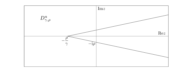
Figure 1: Unstable domain

Let $\tilde{\phi}_{0}$ be defined by (31) in the trigonometric case and $\tilde{\phi}_{0}\equiv 0$ in the polynomial case. Let $\phi_{0}$ be the truncation up to order $n$ in $z^{-r}$ of the formal solution provided by Proposition 3.2, that is, if $n=2m$ with $m\geq 1$,

$$\phi_{0}(z)=\tilde{\phi}_{0}(z)+\sum_{k=1}^{n}c_{k-1}(\mu)z^{-kr},$$ (35)

and, if $n=2m-1$ with $m\geq 2$, $\phi_{0}$ in the polynomial case is

$$\phi_{0}(z)=\sum_{k=1}^{n}\frac{1}{z^{kr}}\sum_{0\leq j\leq\left[\frac{k-1}{m-1}\right]}c_{k-1,j}(\mu)\log^{j}z$$ (36)

and in the trigonometric case

$$\phi_{0}(z)=\tilde{\phi}_{0}(z)+\sum_{k=1}^{n}\frac{1}{z^{kr}}\sum_{0\leq j\leq\left[\frac{k}{m-1}\right]}c_{k-1,j}(\mu)\log^{j}z.$$ (37)

Theorem 3.3.

(Existence theorem) Let $r=2/(n-1)$ and $c_{0}$ be such that $c_{0}^{n-1}=-r(r+1)$. For any $\gamma>0$ there exists $\rho_{0}$ big enough such that for any $\rho\geq\rho_{0}$, the inner equations (27) and (28) have two analytic solutions $\phi^{{\rm u},{\rm s}}:D_{\gamma,\rho}^{{\rm u},{\rm s}}\times B(\mu_{0})\to\mathbb{C}$ such that

$$\phi^{{\rm u},{\rm s}}(z,\mu)=\phi_{0}(z)+\psi^{{\rm u},{\rm s}}(z,\mu),$$

with

$$\sup_{(z,\mu)\in D_{\gamma,\rho}^{{\rm u},{\rm s}}\times B(\mu_{0})}|z^{r+2}\psi^{{\rm u},{\rm s}}(z,\mu)|<+\infty,$$

Now we state the theorem for the difference $\phi^{{\rm u}}-\phi^{s}$. First we define the complex domain (see Figure 2)

$$E_{\gamma,\rho}=D_{\gamma,\rho}^{{\rm u}}\cap D_{\gamma,\rho}^{{\rm s}}\cap\{z\in\mathbb{C}:\text{Im}z<0\}\backslash\{z\in\mathbb{C}:|\text{Re}z|\leq 1,\;|\text{Im}z|\leq\rho+\gamma\},$$ (38)

where the difference between two solutions of the inner equation (27) $\phi^{{\rm u}}-\phi^{{\rm s}}$ is defined.

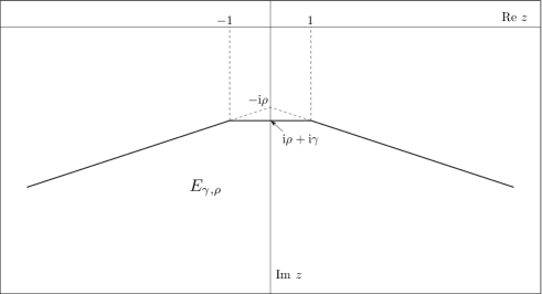
Figure 2: Inner Domain

To unify the notation we introduce the new parameters

$$\ell=\left\{\begin{array}[]{cl}r+2&\text{polynomial case}\\ 2&\text{trigonometric case}\end{array}\right.,\;\;\;\;\;d_{\ell}=\left\{\begin{array}[]{cl}c_{0}&\text{polynomial case}\\ 1&\text{trigonometric case}\end{array}\right.$$ (39)

Theorem 3.4.

Let $\phi^{{\rm u},{\rm s}}$ be two analytic solutions of equations (27) and (28) satisfying the conditions stated in Theorem 3.3.

Their difference $\phi^{{\rm u}}-\phi^{{\rm s}}:E_{\gamma,\rho}\times B(\mu_{0})\to\mathbb{C}$, can be expressed as

$$\phi^{{\rm u}}(z,\mu)-\phi^{{\rm s}}(z,\mu)=\zeta_{1}(z,\mu)\sum_{k<0}p_{k}^{1}(\mu)\text{e}^{2\pi\text{i}kz}+\zeta_{2}(z,\mu)\sum_{k<0}p_{k}^{2}(\mu)\text{e}^{2\pi\text{i}kz}$$ (40)

with $p_{k}^{1},p_{k}^{2}$ analytic functions in $B(\mu_{0})$ and $\zeta_{1},\zeta_{2}$ satisfying that:

1. their wronskian

   $$W(\zeta_{1},\zeta_{2}):=\left|\begin{array}[]{cc}\zeta_{1}(z,\mu)&\zeta_{2}(z,\mu)\\ \zeta_{1}(z+1,\mu)&\zeta_{2}(z+1,\mu)\end{array}\right|=1$$

2. there exists a constant $C$ such that for any $z\in E_{\gamma,\rho}$ and $\mu\in B(\mu_{0})$,

   $$\big{|}z^{1-\ell}\text{e}^{2\pi\text{i}z}\big{(}\zeta_{1}(z,\mu)-\partial_{z}\phi^{{\rm s}}(z,\mu)\big{)}\big{|}\leq C,\;\;\;\;\;\left|\frac{z^{-\nu}}{\log^{\sigma}z}\left(\zeta_{2}(z,\mu)-\frac{z^{\ell}}{rd_{\ell}(2\ell-1)}\right)\right|\leq C$$

   with $\nu=\ell-r$, $\sigma=0$ if $n>3$, $\nu=\ell-1$ if $n\leq 3$, $\sigma=0$ if $n=2$ and $\sigma=1$ if $n=3$.

From now on we will skip the dependence on $\mu$ being always analytic.

4 Numerical results

In this section we present some numerical results concerning the generalized standard map (5) given by the functions $f_{1}(x,h)=\varepsilon(x-x^{3})-\varepsilon^{2}x^{7}$ in (14) and $f_{2}(x,h)=\varepsilon(x-x^{3})$. We recall here that $\varepsilon=4\sinh^{2}(h/2)$.

We notice that both functions $f_{1},f_{2}$ satisfy the hypotheses of Section 2.5. Henceforth, as we show in Section 2.5.1, we can construct the inner equation for the generalized standard map induced by them:

$$\Delta^{2}(\phi)=-\phi^{7}\;\;\;\;\;\text{and}\;\;\;\;\;\Delta^{2}(\phi)=-\phi^{3}.$$ (41)

The first one corresponds to $f_{1}$ and the second one to $f_{2}$.

Let

$$\Theta:=\phi^{{\rm u}}-\phi^{{\rm s}},$$

be the difference between the two solutions of the inner equation (41) given by Theorem 3.3. First of all, in a general setting, we relate the main term of $\Theta$ with the Lazutkin invariant for the standard map (5) induced by $f$. Next, we compute the actual Lazutkin invariant for the maps defined by $f_{1}$ and $f_{2}$ which is computed numerically by using multiprecision routines. After we summarize the method to compute the main term of the difference $\Theta:=\phi^{{\rm u}}-\phi^{{\rm s}},$ by exploiting the theoretical framework we have developed. One aspect worth to remark is that these computations have been performed through standard long double precision arithmetic.

A similar, but more detailed, numerical comparison between the Lazutkin invariant and the difference $\Theta$ is performed in [GG11] for the Swift-Hohenberg equation.

4.1 The relation between the Lazutkin invariant and $\Theta$

For computing the first asymptotic term of $\Theta$ we now take advantage from the fact that we have an alternative expression for $\Theta$ by using the functions $\zeta_{1}$ and $\zeta_{2}$ given in Theorem 3.4. Indeed, we actually can write the difference $\Theta$ as

$$\Theta(z)=\zeta_{1}(z)\sum_{k<0}p_{k}^{1}\text{e}^{2\pi\text{i}kz}+\zeta_{2}(z)\sum_{k<0}p_{k}^{2}\text{e}^{2\pi\text{i}kz}$$

with $p_{j}(z)=\sum_{k<0}p_{k}^{j}\text{e}^{2\pi\text{i}kz}$, $j=1,2$ $1$-periodic functions. We recall that by Theorem 3.4 $W(\zeta_{1},\zeta_{2})=1$ and henceforth $p_{1}=W(\Theta,\zeta_{2})$ and $p_{2}=W(\zeta_{1},\Theta)$.

On the one hand, we introduce the new quantity $\omega_{{\rm in}}(z)$:

$$\omega_{{\rm in}}(z):=-\frac{d}{dz}W(\Theta,\zeta_{1})(z)=\frac{d}{dz}p_{2}(z)=\sum_{k<0}2\pi\text{i}kp_{k}^{2}\text{e}^{2\pi\text{i}kz}\thickapprox-2\pi\text{i}p_{-1}^{2}\text{e}^{-2\pi\text{i}z}.$$ (42)

The last equality has been deduced as $\text{Im}z\to-\infty$. On the other hand, note that by using the first approximations of $\zeta_{1}$ and $\zeta_{2}$ in Theorem 3.4, since $\ell>0$, $\zeta_{1}(z)\to 0$ as $\text{Im}z\to-\infty$ and $\zeta_{2}(z)=\mathcal{O}(z^{\ell})$, the main term of $\Theta$ is

$$\Theta(z)=\zeta_{1}(z)p_{1}(z)+\zeta_{2}(z)p_{2}(z)\thickapprox\zeta_{2}(z)p_{2}(z)\thickapprox z^{\ell}\frac{p_{-1}^{2}}{rd_{\ell}(2\ell-1)}\text{e}^{-2\pi iz}.$$

We recall here that only $p_{-1}^{2}$ is unknown, the other quantities are defined in terms of the inner equation. Henceforth, both $\omega_{{\rm in}}(z)$ and $z^{-\ell}\Theta(z)$, are asymptotically equivalent.

In order to compare the numerical results with our theoretical framework we will gather in a rather informal way several facts, some of them not proven. In particular, to transform assumptions (A1) and (A2) below into proven facts would require involved arguments even for particular cases. By this reason, we will avoid precise statements. The chain of reasoning is a slight modification of the one in [MSS11a], which also follows [Laz03, Gel99].

Let $f$ be a real analytic function satisfying the hypotheses in Section 2.1 and Section 2.5. We first remark that there exists a solution of the invariance equation (9) induced by $f$, $x^{{\rm u}}(t)$, $\text{i}\pi$-antiperiodic, entire and real analytic in $t$, such that $\lim_{\text{Re}t\to-\infty}x^{{\rm u}}(t)=0$ and $x^{{\rm u}}(0)=x^{{\rm u}}(-h)$ (and $x^{{\rm u}}(t)-x^{{\rm u}}(t-h)>0$, for $t\leq 0$). Then, the function $x^{{\rm s}}(t)=x^{{\rm u}}(-t)$ is also a solution of (9), with the same regularity, satisfying $\lim_{\text{Re}t\to\infty}x^{{\rm s}}(t)=0$. Hence, $\gamma^{{\rm u},{\rm s}}(t)=(x^{{\rm u},{\rm s}}(t),x^{{\rm u},{\rm s}}(t)-x^{{\rm u},{\rm s}}(t-h))$ are natural parametrizations of the invariant manifolds of the origin. We notice that $p=\gamma^{{\rm u}}(0)=\gamma^{{\rm s}}(0)=(x^{{\rm u},{\rm s}}(0),0)$ is the first homoclinic point. Let $D(t)=x^{{\rm s}}(t)-x^{{\rm u}}(t)$.

Using the $h$-step Wronskian

$$W_{h}(u,v)(t)=\begin{vmatrix}u(t)&v(t)\\ u(t)-u(t-h)&v(t)-v(t-h)\end{vmatrix}=\begin{vmatrix}u(t)&v(t)\\ \Delta_{h}u(t)&\Delta_{h}v(t)\end{vmatrix}$$

the Lazutkin invariant (11) can be written as

$$\omega(p)=\det(\dot{\gamma}^{u},\dot{\gamma}^{s})_{\mid t=0}=\frac{d}{dt}\det(\dot{\gamma}^{u},\gamma^{s}-\gamma^{u})_{\mid t=0}=\frac{d}{dt}W_{h}(\dot{x}^{u},D)_{\mid t=0}.$$ (43)

Since both $x^{u}$ and $x^{s}$ are solutions of the second order difference equation (9), their difference $D$ also satisfies a linear second order equation, namely

$$\Delta_{h}^{2}D(t)=-\left(\int_{0}^{1}\frac{\partial}{\partial x}f(sx^{{\rm s}}(t)+(1-s)x^{{\rm u}}(t),h)\,ds\right)D(t).$$ (44)

Notice that, if $x^{{\rm u}}$ is close to $x^{{\rm s}}$, then equation (44) is close to the linearization of the invariance equation (9) around $x^{{\rm u}}$. Hence, our first assumption is that

1. there is a (real analytic) solution $\eta_{1}$ of equation (44) close to $\dot{x}^{{\rm u}}$.

Let $\eta_{2}$ be another (real analytic) solution of (44) with $W_{h}(\eta_{1},\eta_{2})=1$, which can be obtained by the “variation of constants” method. Hence, we can write $D=c_{1}\eta_{1}+c_{2}\eta_{2}$ where $c_{1}$ and $c_{2}$ are the $h$-periodic functions $c_{1}=W_{h}(D,\eta_{2})$ and $c_{2}=W_{h}(\eta_{1},D)$. Substituting this expression for $D$ into (43) and using that $\eta_{1}$ is close to $\dot{x}^{u}$ we have that

$$\omega(p)\thickapprox\frac{d}{dt}W_{h}(\eta_{1},D)_{\mid t=0}.$$ (45)

Since $f$ satisfies the hypotheses of Section 2.5, we can construct an inner equation associated to the standard map induced by$f$. The second assumption is

1. there exists $\chi\in\mathbb{C}$ (which can depend on $h$) such that for values of $t$ satisfying $|t-\chi|=\mathcal{O}(h)$, $x^{{\rm u},{\rm s}}(t)$ are close to $h^{-\alpha}\lambda\phi^{{\rm u},{\rm s}}((t-\chi)/h)$. Here $\phi^{{\rm u},{\rm s}}$ are the solutions of the inner equation (27) given by Theorem 3.3 and $\alpha,\lambda$ are both parameters introduced in Section 2.5. Since $f$ is real analytic one can assume that $\text{Im}\chi>0$.

As a consequence, since, by Theorem 3.4, $\zeta_{1}(z)=\partial_{z}\phi^{{\rm u}}(z)+\mathcal{O}(z^{r+1}\text{e}^{2\pi\text{i}z})$,

$$\dot{x}^{{\rm u}}(t)\thickapprox h^{-\alpha-1}\lambda\frac{d}{dz}\phi^{{\rm u}}((t-\chi)/h)\thickapprox h^{-\alpha-1}\lambda\zeta_{1}((t-\chi)/h).$$

Recall now that $p_{2}(z)=-W(\Theta,\zeta_{1})(z)$. Hence, taking into account the scaling and assumption (A1), for values of $t$ close to $\chi$,

$$W_{h}(\eta_{1},D)(t)\thickapprox W_{h}(h^{-\alpha-1}\lambda\zeta_{1},h^{-\alpha}\lambda\Theta)((t-\chi)/h)=h^{-2\alpha-1}\lambda^{2}p_{2}\big{(}(t-\chi)/h\big{)}.$$

Then, since $W_{h}(\eta_{1},D)(t)$ and $W(\zeta_{1},\Theta)((t-\chi)/h\big{)}$ are both $h$-periodic and that the first one is a real analytic function we easily have that, for real $t$

$$\frac{d}{dt}W_{h}(\dot{x}^{{\rm u}},D)(t)\thickapprox 2h^{-2\alpha-2}\text{Re}\left(\lambda^{2}\cdot\frac{d}{dz}p_{2}\big{(}(t-\chi)/h\big{)}\right)=2h^{-2\alpha-2}\text{Re}\left(\lambda^{2}\cdot\omega_{{\rm in}}\big{(}(t-\chi)/h\big{)}\right)$$

with $\omega_{{\rm in}}$ defined in (42). Hence, evaluating at $t=0$,

$$\omega(p)\thickapprox 2h^{-2\alpha-2}\text{Re}\left(\lambda^{2}\cdot\omega_{{\rm in}}(-\chi/h)\right).$$ (46)

Our goal now is to check numerically the above formula for the maps induced by $f_{1}$ and $f_{2}$.

4.2 The limit flow and its singularities

In the cases of the Chirikov standard map and the perturbations of the McMillan map in [Gel99] and [MSS11a], resp, $\chi=\text{i}\pi/2$ is the closest to the real line singularity of the homoclinic orbit of the limit flow (10). In the maps induced by $f_{1}(x,h)=\varepsilon(x-x^{3})-\varepsilon^{2}x^{7}$ and $f_{2}(x,h)=\varepsilon(x-x^{3})$ under consideration, the closest to the real line singularity of the homoclinic of the limit flow $\ddot{x}=x-x^{3}$ is also $\text{i}\pi/2$ (see Section 2.4). Nevertheless, our numerical computations show that it is not the right guess for $\chi$ in the case of $f_{1}$. For this reason, we consider the higher order (in $h$) limit flow

$$\ddot{x}=x-x^{3}-\varepsilon x^{7}.$$ (47)

The parametrization, $x_{0}(t,h)$, of the homoclinic loop to the origin such that $\dot{x}_{0}(0,h)=0$ has a singularity at

$$\rho(h)=\int_{x_{0}(0,h)}^{+\infty}\frac{dx}{\sqrt{x^{2}/2-x^{4}/4-\varepsilon x^{8}/8}},$$

where $x_{0}(0,h)=\sqrt{2}+O(h^{2})$ is the positive root of $x^{2}/2-x^{4}/4-\varepsilon x^{8}/8$ and the integral is computed along the real line. The other singularities can be obtained changing the path of integration. It can be seen that

$$\rho(h)=\text{i}\frac{\pi}{2}-\text{i}\frac{2^{1/4}\Gamma(3/4)^{2}}{\sqrt{\pi}}h^{1/2}+O(h^{3/2}).$$ (48)

We remark that, although the singularities of the homoclinic of (47) tend to the singularities of the limit flow $\ddot{x}=x-x^{3}$ (10) (in a rather slow way), they are of a different type: whereas the latter are poles, the former are branching points.

We choose the values $\chi=\text{i}\frac{\pi}{2}-\text{i}\frac{2^{1/4}\Gamma(3/4)^{2}}{\sqrt{\pi}}h^{1/2}$ for $f_{1}$ and $\chi=\text{i}\frac{\pi}{2}$ for $f_{2}$ and we will assume that (i) holds for them.

4.3 Numerical computations

We define now

$$\tilde{\omega}(h)=h^{2\alpha+2}\lambda^{-2}\text{e}^{2\pi|\chi|/h}\omega(p),\;\;\;\;\;\;\tilde{\omega}_{{\rm in}}(z)=2\text{e}^{2\pi\text{i}z}\text{Re}\left(\omega_{{\rm in}}(z)\right)$$ (49)

taking $\lambda=1$ and on the one hand $\alpha=2/3$ for $f_{1}$ and on the other hand $\alpha=1$ for $f_{2}$. We note that, since $\chi$ has no real part, checking formula (46) is equivalent to check that

$$\tilde{\omega}(h)\thickapprox\tilde{\omega}_{{\rm in}}\big{(}-\chi/h\big{)}\Leftrightarrow\lim_{h\to 0}\tilde{\omega}(h)=\lim_{\text{Im}z\to-\infty}\tilde{\omega}_{{\rm in}}(z).$$

First we show the results for $\tilde{\omega}(h)$. We have computed numerically this quantity by using multiprecision routines written in PARI-GP. In the following figure we show the computed values for $f_{1}(x,h)=\varepsilon(x-x^{3})-\varepsilon^{2}x^{7}$ and for the map induced by $f_{2}(x,h)=\varepsilon(x-x^{3})$. Let us denote by $\tilde{\omega}_{i}(h)$ the value of $\tilde{\omega}(h)$ for the corresponding maps $f_{i}$, $i=1,2$. We have added a correction factor ${\rm esc}=85\cdot 10^{-4}$ in order to have the same magnitude for both values of $\tilde{\omega}(h)$.

These numbers have been obtained computing explicitly $\omega(p)=\det({\dot{\gamma}}^{u}(0),\dot{\gamma}^{s}(0))$, following the strategy in [DRR99]. Due to the exponentially small behavior of this quantity, it has been necessary to compute $\dot{\gamma}^{u,s}(0)$ with increasing accuracy, thus making impossible to achieve very small values of $h$.

Notice that, in the case of the map induced by $f_{2}(x,h)=\varepsilon(x-x^{3})$, the values of $\tilde{\omega}_{2}(h)$ converge quite fast, when $h$ becomes smaller, to a constant value

$$\tilde{\omega}_{2}(h)\thickapprox 1.00083\cdot 10^{5}$$ (50)

In the case of the map induced by $f_{1}(x,h)=\varepsilon(x-x^{3})-\varepsilon^{2}x^{7}$, the convergence of the values of $\tilde{\omega}_{1}(h)$ is slower, as the previous figure shows. However, computing $\tilde{\omega}_{1}(h)$ for $h=1/2000+k/40000$, $k=0\dots 199$, and making some assumptions on the form of the asymptotic expansion of $\tilde{\omega}_{1}(h)$ in $h$, it is possible to extrapolate the limit value with better accuracy.

In this way, we have obtained that it is

$$\tilde{\omega}_{1}(h)\thickapprox 871.683$$ (51)

We remark that, with the computed data, in which each value of $\tilde{\omega}_{i}(h)$, $i=1,2$, has a few hundreds of correct digits, it would be possible to obtain a better approximation of this value, and also to compute the coefficients of the asymptotic expansion. Since our intention was to compare the results obtained by the analysis of the solutions of the inner equation, we have not pursued in this direction.

Now we compute $\tilde{\omega}_{{\rm in}}(z)$ . By definition (42) of $\omega_{{\rm in}}(z)$ and (25) of the operator $\Delta$,

$$\tilde{\omega}_{{\rm in}}(z)=4\pi\text{e}^{2\pi\text{i}z}\text{Re}\big{(}\Theta(z)\cdot\Delta(\partial_{z}\phi^{{\rm s}})(z)-\partial_{z}\phi^{{\rm s}}(z)\cdot\Delta(\Theta)(z)\big{)}+\mathcal{O}(\text{e}^{-2\pi\text{i}z}z^{2r+2},\text{e}^{-2\pi\text{i}z}),$$ (52)

where we have used that by Theorem 3.4, $\zeta_{1}(z)-\partial_{z}\phi^{{\rm u}}(z)=\mathcal{O}(\text{e}^{-2\pi\text{i}z}z^{r+1})$.

For symmetry reasons, we choose $z=-i\rho$ with $\rho\in[2.25,7]$. We have used long double precision in C for calculating $\phi^{{\rm s},{\rm u}}(z),\partial_{z}\phi^{{\rm s},{\rm u}}(z)$ . The strategy was suggested in [GL01]

• First we compute the formal series $\widetilde{\phi}_{N}$ up to order $N$ big enough. We know that the solutions $\phi^{{\rm s},{\rm u}}$ are close to $\widetilde{\phi}_{N}$ if $|z|$ is big enough. Analogously for $\partial_{z}\phi^{{\rm s},{\rm u}}$.

• We evaluate the formal series $\widetilde{\phi}_{N}(z\pm k)$ and $\partial_{z}\widetilde{\phi}_{N}(z\pm k)$ with $k\in\mathbb{N}$ big enough.

• Since both $\phi^{{\rm s},{\rm u}}$ satisfy the inner equation, we obtain $\phi^{{\rm s},{\rm u}}(z)$ and $\phi^{{\rm s},{\rm u}}(z+1)$ recurrently. Analogously for $\partial_{z}\phi^{{\rm s},{\rm u}}(z)$ and $\partial_{z}\phi^{{\rm s},{\rm u}}(z+1)$

We have computed $\tilde{\omega}_{{\rm in}}(z)$ for the inner equations (41). Our results are given in the following picture, where we have added the scaling factor ${\rm esc}=871\cdot 10^{-5}$.

We can observe that, on the one hand when $\text{Im}z\in[-3,-2]$ the theoretical error in (52) is big. On the other hand, when $\text{Im}z\in[-7,-6]$ the round-off errors (for $f_{1}$) begin to be bigger than the theoretical error and hence the computed values have noise. Nevertheless for values of $\text{Im}z\in[-5,-3]$ the computed values of $\tilde{\omega}_{{\rm in}}(z)$ behave like a constant. More precisely, we have found $\tilde{\omega}_{{\rm in}}(z)=871.6833\dots$ for $\Delta^{2}(\phi)=-\phi^{7}$ and $\tilde{\omega}_{{\rm in}}(z)=1.000832\dots 10^{5}$ for $\Delta^{2}(\phi)=-\phi^{3}$ which agree with the results for $\tilde{\omega}(h)$ given in (50) and (51).

5 Formal solutions of the inner equation

In this section we prove the existence of formal solutions of the inner equation (27). The proof of the existence of formal solutions of equation (28) follows the same procedure. Hence, we skip it.

We start by defining the spaces which these formal solutions belong to. For $n\in\mathbb{N}$ and $r(n-1)=2$, we define

$$X_{r}=\Big{\{}\phi(z)=\sum_{k\geq 1}\frac{c_{k-1}}{z^{kr}}|\;c_{k}\in\mathbb{C}\Big{\}},$$ (53)

the space of formal power series in $x^{-r}$ without constant term, and, if $n=2m-1$, $m\geq 2$, that is, $r=1/(m-1)$,

$$X_{r}^{\log}=\Big{\{}\phi(z)=\sum_{k\geq 1}\sum_{0\leq j\leq\left[\frac{k-1}{m-1}\right]}c_{k-1,j}\frac{\log^{j}z}{z^{kr}}|\;c_{k,j}\in\Big{\}},$$ (54)

where $[x]$ denotes the integer part of $x$, the space of formal power series in $x^{-r}$ and $\log z$, with the power of $\log z$ bounded by the power of $x^{-r}$, without constant term.

We will say that $\phi=\mathcal{O}_{kr}$, with $k\in\mathbb{N}$, if and only if $z^{kr}\phi\in\mathbb{C}[[z^{-r}]]$ is a power series with terms $z^{-jr}$ for $j\geq 0$. We will also use $\mathcal{O}_{kr,j}$ in $X_{r}^{\log}$, with $k\in\mathbb{N}$, $j\in\mathbb{N}\cup\{0\}$, meaning that $\phi=\mathcal{O}_{kr,j}$ implies that $z^{kr}(\log z)^{-j}\phi(z)$ is a formal power series with terms of the form $z^{-k^{\prime}r}\log^{j^{\prime}}z$, with $k^{\prime}\geq 0$ and $j^{\prime}\geq-j$ such that $j^{\prime}\leq 0$ whenever $k^{\prime}=0$. We keep both notations in order to emphasize that $\mathcal{O}_{kr}$ is a series without logarithms, while $\mathcal{O}_{kr,0}$ is a series whose leading term does not have logarithms.

We collect several properties of these spaces in the following lemma, whose proof is straightforward.

Lemma 5.1.

Let $n\geq 2$, $r=2/(n-1)$ and $g$ an analytic function around the origin with $g(y)=Ay^{\ell}+\mathcal{O}(y^{\ell+1})$, for some $\ell\in\mathbb{N}\cup\{0\}$. The spaces $X_{r}$, for $n$ even, and $X_{r}^{\log}$, for $n$ odd, have the following properties:

1. $X_{r}$ and $X_{r}^{\log}$ are invariant by the formal differential operator $\frac{\partial^{2}}{\partial z^{2}}$. Furthermore, if $\phi\in X_{r}^{\log}$ (resp. $X_{r}$), then $\frac{\partial^{2}}{\partial z^{2}}\phi(z)=z^{-2}\psi(z)$ with $\psi\in X_{r}^{\log}$ (resp. $X_{r}$).

2. If $\phi(z)=az^{-r}+\tilde{\phi}(z)$, with $\tilde{\phi}=\mathcal{O}_{2r,j}$, $0\leq j\leq[1/(m-1)]$, resp. $\mathcal{O}_{2r}$, then $g(az^{-r}+\tilde{\phi}(z))=Aa^{\ell}z^{-\ell r}+\varphi(z)$, with $\varphi=\mathcal{O}_{(\ell+1)r,j}$, resp. $\mathcal{O}_{(\ell+1)r}$.

Moreover, in the case $n=2m-1$, $X_{r}^{\log}$ is also invariant by translation, that is, if $\phi(z)\in X_{r}^{\log}$, then $\phi(z-c)\in X_{r}^{\log}$, for any $c\in\mathbb{C}$. In the case $n=2m$, if $\phi\in X_{r}$, then $\phi(z-c)\in X_{r/2}$.

We recall the function $g(y)=y^{n}-G(y)$. We remark that, since the operator $\Delta^{2}$ can be written formally as

$$\Delta^{2}\phi(z)=4\sinh^{2}\left(\frac{1}{2}\frac{\partial}{\partial z}\right)\phi(z)=\left(\frac{\partial^{2}}{\partial z^{2}}+\frac{1}{12}\frac{\partial^{4}}{\partial z^{4}}+\cdots\right)\phi(z),$$ (55)

(1) in Lemma 5.1 implies that the inner equation (27) is well defined in $X_{r}$ and $X_{r}^{\log}$. We introduce

$$\epsilon(\phi)=\Delta^{2}(\phi)-g(\phi).$$ (56)

It is clear that $\epsilon(\phi)(z)=z^{-2}\hat{\epsilon}(z)$ with $\hat{\epsilon}\in X_{r}^{\log}$ (resp. $X_{r}$).

Next lemma follows directly from the definition of $X_{r}^{\log}$.

Lemma 5.2.

Let $n=2m-1$, $r=1/(m-1)$ and $\phi\in X_{r}^{\log}$ and $\epsilon(\phi)$ as in (56). If $z^{2}\epsilon(\phi)(z)$ has no terms of order $N$ or smaller in $z^{-r}$ (that is, no terms of the form $z^{-kr}\log^{j}z$, with $1\leq k\leq N$), then $\epsilon(\phi)=\mathcal{O}_{(N+1)r+2,L}$, where $L=[N/(m-1)]$.

Definition 5.3.

Let $n\geq 2$, $N\in\mathbb{N}$, $r=2/(n-1)$ and $\phi\in X_{r}$ or $X_{r}^{\log}$. We will call truncated series of order $N$ of $\phi$ to $\tilde{\phi}_{N}$ having the form:

1. If $n$ is even,

   $$\tilde{\phi}_{N}(z)=\sum_{k=1}^{N}\frac{c_{k-1}}{z^{kr}}$$

2. If $n=2m-1$ is odd,

   $$\tilde{\phi}_{N}(z)=\sum_{k=1}^{m-1}\frac{c_{k-1}}{z^{kr}}+\sum_{k=m}^{N}\frac{1}{z^{kr}}\sum_{0\leq j\leq\left[\frac{k-1}{m-1}\right]}c_{k-1,j}\log^{j}z.$$

Along the proof of Proposition 3.2, we will need to compute several times the formal series $g(\phi+\psi)-g(\phi)$, with different $\phi$ and $\psi$. The following lemma, which follows from the properties in Lemma 5.1, summarizes the result.

Lemma 5.4.

Let $n\geq 2$, $r=2/(n-1)$, $N\geq 2$, $N\in\mathbb{N}$ and $\phi\in X_{r}$ or $X_{r}^{\log}$. We define $\psi_{N}=\tilde{\phi}_{N}-\tilde{\phi}_{N-1}$ where $\tilde{\phi}_{N}$ and $\tilde{\phi}_{N-1}$ are the truncated series of order $N$ and $N-1$ respectively. We have that

1. If $n$ is even,

   $$g(\tilde{\phi}_{N}(z))-g(\tilde{\phi}_{N-1}(z))=-n\frac{c_{0}^{n-1}}{z^{2}}\psi_{N}(z)+\mathcal{O}_{(N+1)r+2}.$$

2. If $n=2m-1$ is odd, writing $L=[N/(m-1)]$,

   $$g(\tilde{\phi}_{N}(z))-g(\tilde{\phi}_{N-1}(z))=-n\frac{c_{0}^{n-1}}{z^{2}}\psi_{N}(z)+\mathcal{O}_{(N+1)r+2,L}.$$

The following proposition implies the existence of formal solution of the inner equation (27) and henceforth Proposition 3.2.

Proposition 5.5.

Let $n\geq 2$, $r=2/(n-1)$ and $c_{0}$ be such that $c_{0}^{n-1}=-r(r+1)$. The inner equation (27) admits a formal solution $\phi$ with $z^{r}(\phi(z)-c_{0}z^{-r})\in X_{r}$, if $n$ is even, and $z^{r}(\phi(z)-c_{0}z^{-r})\in X_{r}^{\log}$ if $n$ is odd.

Let $N\geq 2$ and $\tilde{\phi}_{N}$ be the truncated series defined as in Definition 5.3. Writing the truncation error of order $N$ as

$$\epsilon_{N}:=\epsilon(\tilde{\phi}_{N})=\Delta^{2}(\tilde{\phi}_{N})-g(\tilde{\phi}_{N}),$$

where $\epsilon$ was defined by (56), we have that

1. If $n\geq 2$ is even $\epsilon_{N}=\mathcal{O}_{(N+1)r+2}$.

2. If $n=2m-1\geq 2$ is odd and $L=[N/(m-1)]$, then

   1. if $1\leq N\leq m-1$, $\epsilon_{N}=\mathcal{O}_{(N+1)r+2}$,

   2. if $m\leq N$, $\epsilon_{N}=\mathcal{O}_{(N+1)r+2,L}$.

Proof.

We deal first with 1). We prove the claim by induction over $N$. We start by assuming $N=1$. Let $\tilde{\phi}_{1}(z)=c_{0}z^{-r}$. By (2) in Lemma 5.1 and using (55), we have that

$$\epsilon_{1}(z)=\Delta^{2}(\tilde{\phi}_{1})(z)-g(\tilde{\phi}_{1}(z))=r(r+1)\frac{c_{0}}{z^{r+2}}+\frac{c_{0}^{n}}{z^{nr}}+\mathcal{O}_{(n+1)r}.$$

The claim for $N=1$ follows from the facts that $r=2/(n-1)$, which implies $\mathcal{O}_{(n+1)r}=\mathcal{O}_{2r+2}$, and $c_{0}^{n-1}=-r(r+1)$.

Now we assume the claim for $N-1$, that is, there exist coefficients $c_{k}$, $1\leq k\leq N-2$ such that $\tilde{\phi}_{N-1}$ satisfies

$$\epsilon_{N-1}(z)=\epsilon(\tilde{\phi}_{N-1})(z)=\frac{A_{N-1}}{z^{Nr+2}}+\mathcal{O}_{(N+1)r+2}.$$

We look for $\tilde{\phi}_{N}(z)=\tilde{\phi}_{N-1}(z)+c_{N-1}z^{-Nr}$ satisfying the claim. We have that

$$\epsilon_{N}(z)=\epsilon_{N-1}(z)+\Delta^{2}\left(\frac{c_{N-1}}{z^{Nr}}\right)-g\left(\tilde{\phi}_{N-1}(z)+\frac{c_{N-1}}{z^{Nr}}\right)+g(\tilde{\phi}_{N-1}(z))$$

By 1) of Lemma 5.4,

$$g\left(\tilde{\phi}_{N-1}(z)+\frac{c_{N-1}}{z^{Nr}}\right)-g(\tilde{\phi}_{N-1}(z))=-n\frac{c_{0}^{n-1}}{z^{2}}\frac{c_{N-1}}{z^{Nr}}+\mathcal{O}_{(N+1)r+2}.$$ (57)

Hence, using again (55),

$$\epsilon_{N}(z)=\frac{A_{N-1}}{z^{Nr+2}}+\lambda_{N}\frac{c_{N-1}}{z^{Nr+2}}+\mathcal{O}_{(N+1)r+2},$$

where the coefficient $\lambda_{N}$ is

$$\lambda_{N}=Nr(Nr+1)+nc_{0}^{n-1}=\frac{4}{(n-1)^{2}}\left(N-\frac{n+1}{2}\right)(N+n).$$ (58)

Clearly, the claim follows if $\lambda_{N}$ is different from $0$, which is true since $n$ is even and positive.

Now we assume $n=2m-1$, $m\geq 2$. The induction process used in the previous case can performed provided that $\lambda_{N}\neq 0$. This is true for $N\neq m$. Hence, the claim holds for $1\leq N\leq m-1$. Let $\tilde{\phi}_{m-1}(z)=c_{0}/z^{r}+\dots+c_{m-2}/z^{(m-1)r}$ be the corresponding function. It satisfies,

$$\epsilon_{m-1}(z)=\epsilon(\tilde{\phi}_{m-1})(z)=\frac{A_{m-1}}{z^{mr+2}}+\mathcal{O}_{(m+1)r+2}.$$ (59)

Now we consider the case $N=m$. Since $\lambda_{m}=0$, this case cannot be dealt as before. We need to include logarithms in the formal series.

Notice that, from (55),

$$\Delta^{2}\left(\frac{\log^{\ell}z}{z^{kr}}\right)=kr(kr+1)\frac{\log^{\ell}z}{z^{kr+2}}-{\ell}(2kr+1)\frac{\log^{\ell-1}z}{z^{kr+2}}+{\ell}({\ell}-1)\frac{\log^{\ell-2}z}{z^{kr+2}}+\mathcal{O}_{kr+4,\ell}.$$ (60)

We look for $\tilde{\phi}_{m}=\tilde{\phi}_{m-1}+\psi_{m}$ satisfying the claim, with $\psi_{m}(z)=c_{m-1,1}z^{-mr}\log z+c_{m-1,0}z^{-mr}$. Hence we have that

$$\epsilon_{m}=\epsilon_{m-1}+\Delta^{2}(\psi_{m})-g(\tilde{\phi}_{m-1}+\psi_{m})+g(\tilde{\phi}_{m-1}).$$

From (60), we have that

$$\Delta^{2}(\psi_{m})(z)=\frac{mr(mr+1)}{z^{2}}\psi_{m}(z)-(2mr+1)c_{m-1,1}\frac{1}{z^{mr+2}}+\mathcal{O}_{mr+4,1},$$ (61)

while, from 2) in Lemma 5.4,

$$g(\tilde{\phi}_{m-1}(z)+\psi_{m}(z))-g(\tilde{\phi}_{m-1}(z))=-n\frac{c_{0}^{n-1}}{z^{2}}\psi_{m}(z)+\mathcal{O}_{(m+1)r+2,L},$$ (62)

with $L=[N/(m-1)]=[m/(m-1)]$.

Hence, substituting (61) and (62) into the expression for $\epsilon_{m}$ above, we obtain

$$\epsilon_{m}(z)=\epsilon_{m-1}(z)+\frac{\lambda_{m}}{z^{2}}\psi_{m}(z)-(2mr+1)c_{m-1,1}\frac{1}{z^{mr+2}}+\mathcal{O}_{(m+1)r+2,L},$$

where the coefficient $\lambda_{N}$ was introduced in (58) and, in fact, satisfies $\lambda_{m}=0$. Since $\epsilon_{m-1}(z)=A_{m-1}z^{mr+2}+\mathcal{O}_{(m+1)r+2}$ (see (59)), taking $c_{m-1,1}=A_{m-1}/(2mr+1)$, we have that $\epsilon_{m}=\mathcal{O}_{(m+1)r+2,L}.$ Notice that the coefficient $c_{m-1,0}$ is free. Hence, the claim is proven for $1\leq N\leq m$.

Now proceeding by induction the result is proven. ∎

6 A solution of the inner equation

The goal of this section is to prove the existence of a solution of the inner equation satisfying the properties stated in Theorem 3.3.

For any $\gamma,\rho>0$, we recall the complex domains

$$D_{\gamma,\rho}^{{\rm s}}=\{z\in\mathbb{C}:|\text{Im}z|>-\gamma\text{Re}z+\rho\},\;\;\;\;D_{\gamma,\rho}^{{\rm u}}=-D_{\gamma,\rho}^{{\rm s}}.$$

defined in (34) (see Figure 1). We also introduce the norms

$$\|\varphi\|_{\nu,\gamma,\rho}^{{\rm u},{\rm s}}=\sup_{z\in D_{\gamma,\rho}^{{\rm u},{\rm s}}}|z^{\nu}\varphi(z)|$$

and the Banach spaces

$$\mathcal{X}^{{\rm u},{\rm s}}_{\nu,\gamma,\rho}=\{\varphi:D_{\gamma,\rho}^{{\rm u},{\rm s}}\to\mathbb{C}\;\;\text{such that}\;\;\|\varphi\|_{\nu,\gamma,\rho}^{{\rm u},{\rm s}}<+\infty\}.$$

We also define the functional space

$$\mathcal{X}^{{\rm u},{\rm s}}_{\nu,k,\gamma,\rho}=\{\varphi:D_{\gamma,\rho}^{{\rm u},{\rm s}}\to\mathbb{C}\;\;\text{such that}\;\;\overline{\varphi}(z):=(\log z)^{-k}\varphi(z)\in\mathcal{X}^{{\rm u},{\rm s}}_{\nu,\gamma,\rho}\}$$

and, if there is no danger of confusion, we will simply denote them

$$\mathcal{X}_{\nu}=\mathcal{X}^{{\rm u},{\rm s}}_{\nu,\gamma,\rho},\;\;\;\;\mathcal{X}_{\nu,k}^{\log}=\mathcal{X}^{{\rm u},{\rm s},}_{\nu,k,\gamma,\rho},\;\;\;\;\|\cdot\|_{\nu}=\|\cdot\|_{\nu,\gamma,\rho}^{{\rm u},{\rm s}},\;\;\;\;D_{\gamma,\rho}=D_{\gamma,\rho}^{{\rm u},{\rm s}}.$$

From now on we will denote by $C$ a generic positive constant independent of $\gamma,\rho,\nu$. We state (without proof) the following lemma which will be used without mention along this section.

Lemma 6.1.

Let $0<\nu_{1},\nu_{2}$. For any $\varphi_{1}\in\mathcal{X}_{\nu_{1}}$ and $\varphi_{2}\in\mathcal{X}_{\nu_{2}}$, then

$$\varphi_{1}\cdot\varphi_{2}\in\mathcal{X}_{\nu_{1}+\nu_{2}}\;\;\;\;\;\text{and}\;\;\;\;\;\|\varphi_{1}\cdot\varphi_{2}\|_{\nu_{1}+\nu_{2}}\leq\|\varphi_{2}\|_{\nu_{2}}\cdot\|\varphi_{1}\|_{\nu_{1}}.$$

Also there exists $C>0$ such that if $0<\nu_{1}<\nu_{2}$ and $\varphi\in\mathcal{X}_{\nu_{2}}$, then

$$\varphi\in\mathcal{X}_{\nu_{1}}\;\;\;\;\;\text{and}\;\;\;\;\;\|\varphi\|_{\nu_{1}}\leq C\rho^{-(\nu_{2}-\nu_{1})}\|\varphi\|_{\nu_{2}}.$$

As in previous section, we will denote by $\mathcal{O}_{\nu}$ and $\mathcal{O}_{\nu,k}$ a generic function belonging to $\mathcal{X}_{\nu}$ and $\mathcal{X}_{\nu,k}^{\log}$ respectively.

Theorem 3.3 is rephrased in terms of the Banach spaces $\mathcal{X}_{\nu,\gamma,\rho}^{{\rm u},{\rm s}}$ in the following proposition:

Proposition 6.2.

Given $\gamma>0$, there exists $\rho_{0}>0$ such that for any $\rho\geq\rho_{0}$, the inner equation (27) (polynomial case) and (28) (trigonometric case)

$$\Delta^{2}(\phi)=g(\phi)$$ (63)

have exactly two solutions $\phi^{{\rm u},{\rm s}}$ of the form

$$\phi^{{\rm u},{\rm s}}=\phi_{0}+\psi^{{\rm u},{\rm s}}$$

where $\phi_{0}$ is the truncated series of order $n$ defined in (35), (36) and (37), depending on the case we are dealing with, and $\psi^{{\rm u},{\rm s}}\in\mathcal{X}_{r+2,\gamma,\rho}^{{\rm u},{\rm s}}$.

The properties of $\phi_{0}$ we are interested in follow from Proposition 5.5.

Corollary 6.3.

Let us consider the remainder of order $n$:

$$\epsilon_{0}=\epsilon(\phi_{0})=\Delta^{2}(\phi_{0})-g(\phi_{0})$$

where $\phi_{0}$ is the truncated series of order $n$ defined in (35), (36) and (37).

For any $\gamma>0$ there exists $\rho_{0}$ big enough such that

1. If $n$ is even, $\phi_{0}=c_{0}z^{-r}+\mathcal{O}_{2r}$, in the polynomial case, and $\phi_{0}=\frac{r}{2}\log(-rz^{-2})+\mathcal{O}_{r}$, in the trigonometric one.

2. If $n=2m-1$ is odd, for the polynomial case $\phi_{0}=c_{0}z^{-r}+\mathcal{O}_{2r}+\mathcal{O}_{mr,1}$. Notice that, since $m\geq 2$, in particular we also have that $\phi_{0}=c_{0}z^{-r}+\mathcal{O}_{2r,1}$. In the trigonometric case, we have that $\phi_{0}=\frac{r}{2}\log(-rz^{-2})+\mathcal{O}_{r}+\mathcal{O}_{(m-1)r,1}$ which also implies that $\phi_{0}=\frac{r}{2}\log(-rz^{-2})+\mathcal{O}_{r,1}$.

3. For any value of $n$ we have that $\epsilon_{0}\in\mathcal{X}_{nr+2}$.

The proof of Proposition 6.2 is performed in two steps. In Section 6.1 we introduce a linear equation which is close to the first order variational equation of (63) with respect to $\phi_{0}$. Such linear equation can be easily inverted in the adequate Banach spaces. Finally, in Section 6.2 we look for $\psi^{{\rm u},{\rm s}}$ as a solution of a suitable fixed point equation.

From now on we will only deal with the $-{\rm u}-$ case, being the $-{\rm s}-$ case analogous. For that reason we will skip $-{\rm u}-$ from our notation.

6.1 The linearized inner equation

We introduce the function

$$H(z)=(1+z^{-1})^{\ell}-2+(1-z^{-1})^{\ell}$$ (64)

for both cases, the polynomial and the trigonometric one with $\ell$ defined in (39). In this section we are going to study the following linear homogeneous second order difference equation:

$$\Delta^{2}(\phi)(z)=H(z)\phi(z).$$ (65)

We recall that the wronskian of two solutions, $\phi_{1},\phi_{2}$ of a linear difference equation is defined as:

$$W(\phi_{1},\phi_{2})(z)=\left|\begin{array}[]{cc}\phi_{1}(z)&\phi_{2}(z)\\ \phi_{1}(z+1)&\phi_{2}(z+1)\end{array}\right|.$$

In addiction, on the one hand, equation (65) has the obvious solution $\eta_{2}(z)=z^{\ell}$ and, on the other hand, it is a well known fact that $\eta_{1}=b\cdot\eta_{2}$ is a solution of (65) if and only if

$$\Delta b(z)=\frac{1}{\eta_{2}(z)\cdot\eta_{2}(z+1)}=\frac{1}{z^{\ell}(z+1)^{\ell}}.$$

One can also deduce that $W(\eta_{1},\eta_{2})\equiv 1$.

We will need a right inverse of the linear operator $\Delta$ defined in appropriate Banach spaces. For this reason we introduce the formal operator

$$\Delta^{-1}(h)(z)=\sum_{k\geq 1}h(z-k)$$ (66)

We emphasize that we are dealing with the unstable case.

Lemma 6.4.

Let $\alpha>0$. For any $\gamma>0$ there exists $\rho_{0}>0$ such that, for any $\rho\geq\rho_{0}$, $\Delta^{-1}:\mathcal{X}_{\alpha+1,\gamma,\rho}\to\mathcal{X}_{\alpha,\gamma,\rho}$ is a right inverse of the operator $\Delta$ defined in (25) with $\|\Delta^{-1}\|\leq C$.

The proof of this lemma is straightforward and can be found in [Gel99].

The first variational around $\phi_{0}$ of the inner equation (63) is given by

$$\Delta^{2}(\phi)=\Delta^{2}(\phi)=Dg(\phi_{0})\phi$$ (67)

and we notice that

$$Dg(\phi_{0})=\left\{\begin{array}[]{ll}-n\phi_{0}^{n-1}+DG(\phi_{0})&\text{polynomial case}\\ -(n-1)\text{e}^{\phi_{0}(n-1)}+DG(\text{e}^{\phi_{0}})\text{e}^{\phi_{0}}&\text{trigonometric case.}\end{array}\right.$$

By using the identities $c_{0}^{n-1}=-r(r+1)$ and $nr=r+2$, the fact that $H(z)=(\ell-1)\ell z^{-2}+\mathcal{O}_{3}$ and Corollary 6.3, the following result follows:

Lemma 6.5.

For any $\gamma>0$ there exists $\rho_{0}>0$ big enough such that

1. The function $H(z)$ satisfies $H=Dg(\phi_{0})-A$, with $A\in\mathcal{X}_{r+2}$, if $n\neq 3$, and $A\in\mathcal{X}_{r+2,1}^{\log}$, if $n=3$,

2. The function $\eta_{2}(z)=z^{\ell}$ is a solution of equation (65). Consequently, the function $\eta_{1}$ defined by

   $$\eta_{1}(z) =z^{\ell}\sum_{k>0}\frac{1}{(z-k)^{\ell}(z-(k+1))^{\ell}},$$

   is also an independent solution with $W(\eta_{1},\eta_{2})=1$. By Lemma 6.4, $\eta_{1}\in\mathcal{X}_{\ell-1}$

We notice that property (1) of Lemma 6.5 implies that the linear equation (65) is a good approximation of the first order variational with respect to $\phi_{0}$ (67).

Finally, as we will see in the lemma below, Lemma 6.5 allows us to invert the linear operator $\mathcal{L}(\phi)(z)=\Delta^{2}(\phi)(z)-H(z)\phi(z)$.

Lemma 6.6.

For any $\gamma>0$, there exists $\rho_{0}>0$ such that for any $\rho\geq\rho_{0}$, the operator $\mathcal{L}(\phi)=\Delta^{2}(\phi)-H\cdot\phi$ has right inverse $\mathcal{L}^{-1}:\mathcal{X}_{\alpha+2,\gamma,\rho}\to\mathcal{X}_{\alpha,\gamma,\rho}$ i if $\alpha>\ell-1$ and it has the expression

$$\mathcal{L}^{-1}(h)=\eta_{1}\cdot\Delta^{-1}(\eta_{2}\cdot h)-\eta_{2}\cdot\Delta^{-1}(\eta_{1}\cdot h).$$ (68)

Moreover, $\|\mathcal{L}^{-1}(h)\|_{\alpha,\gamma,\rho}\leq C\|h\|_{\alpha+2,\gamma,\rho}$ being $C$ an independent constant of $\gamma,\rho$.

Proof.

We will skip $\gamma,\rho$ from the notation. On the one hand $\eta_{1},\eta_{2}$ are independent solutions of the homogeneous linear equation $\mathcal{L}(\phi)=0$ and hence, by the variation of constants method, we obtain formula (68). On the other hand, if $g\in\mathcal{X}_{\alpha+2}$ with $\alpha>\ell-1$, then, $\eta_{2}\cdot g\in\mathcal{X}_{\alpha+2-\ell}$ and $\eta_{1}\cdot g\in\mathcal{X}_{\alpha+\ell+1}$ and by Lemma 6.4, $\eta_{1}\cdot\Delta^{-1}(\eta_{2}\cdot g)\in\mathcal{X}_{\alpha}$ and $\eta_{2}\cdot\Delta^{-1}(\eta_{1}\cdot g)\in\mathcal{X}_{\alpha}$. The bound $\|\mathcal{L}^{-1}(g)\|_{\alpha}\leq C\|g\|_{\alpha+2}$ is obtained by a direct application of Lemma 6.4. ∎

6.2 The fixed point equation

In this section we are going to prove Proposition 6.2 about the existence and properties of solutions of the inner equation (27) (polynomial case) and (28) (trigonometric case)

$$\Delta^{2}(\phi)=-g(\phi)$$

of the form $\phi=\phi_{0}+\psi$, with $\phi_{0}$ given by (35) ($n$ even), (36) ($n$ odd, polynomial case) or (37) ($n$ odd, trigonometric case).

We introduce

$$\epsilon_{0}=-\Delta^{2}(\phi_{0})+g(\phi_{0}),\;\;\;\;\;\;\mathcal{R}(\psi)=\psi^{2}\int_{0}^{1}D^{2}g(\phi_{0}+\lambda\psi)(1-\lambda)\,d\lambda$$ (69)

and we note that if $\phi=\phi_{0}+\psi$ is a solution of the inner equation then, by (1) of Lemma 6.5 $\psi$ has to satisfy the second order difference equation given by

$$\Delta^{2}(\psi)-H\cdot\psi=\epsilon_{0}+A\cdot\psi+\mathcal{R}(\psi)$$ (70)

As we proved in Lemma 6.6, the linear operator $\mathcal{L}$ has a right-inverse in some adequate Banach spaces. Using it, we will obtain a solution of the equation (70) by using the fixed point equation given by

$$\psi=\mathcal{F}(\psi):=\mathcal{L}^{-1}(\epsilon_{0})+\mathcal{L}^{-1}(A\cdot\psi)+\mathcal{L}^{-1}\circ\mathcal{R}(\psi).$$ (71)

Proposition 6.7.

Let $\gamma>0$. There exists $\rho_{1}>0$ big enough such that, for any $\rho\geq\rho_{1}$, the fixed point equation (71) has a unique solution $\psi\in\mathcal{X}_{r+2,\gamma,\rho}$.

Proof.

We first note that there exists $\rho_{0}>0$ such that $\mathcal{L}^{-1}(\epsilon_{0})\in\mathcal{X}_{r+2,\gamma,\rho_{0}}$ since, by Corollary 6.3, $\epsilon_{0}\in\mathcal{X}_{r+4,\gamma,\rho_{0}}$ if $\rho_{0}$ is large enough. Let $\varrho_{0}=2\|\mathcal{L}^{-1}(\epsilon_{0})\|_{r+2,\gamma,\rho_{0}}$. Along the proof of this proposition we will denote by $K$ a generic constant depending only on $\phi_{0}$, $\rho_{0}$ and $\gamma$ and we will omit the dependence on $\gamma$ and $\rho$ in the Banach spaces and norms.

Let $\psi_{1},\psi_{2}\in B(\varrho_{0})\subset\mathcal{X}_{r+2}$. We start by bounding the difference $\|\mathcal{F}(\psi_{1})-\mathcal{F}(\psi_{2})\|_{r+2}$. By Lemma 6.5 we have that, taking $\nu_{r}=0$, if $n\neq 3$, and $\nu_{r}=r/2$, if $n=3$, we have that $A\in\mathcal{X}_{r+2-\nu_{r},\gamma,\rho_{1}}$ provided that $\rho_{1}$ is large enough. Henceforth, if $\psi\in\mathcal{X}_{r+2}$, $A\cdot\psi\in\mathcal{X}_{2r+4-\nu_{r}}$. Applying Lemmas 6.1 and 6.6 we can easily check that

$$\|\mathcal{L}^{-1}(A\cdot(\psi_{1}-\psi_{2}))\|_{r+2}\leq C\rho_{1}^{-r+\nu_{r}}\|A\|_{r+2-\nu_{r}}\cdot\|\psi_{1}-\psi_{2}\|_{r+2}.$$ (72)

Now we deal with $\mathcal{R}(\psi_{1})-\mathcal{R}(\psi_{2})$. We recall that $\mathcal{R}$ was defined in (69). We notice that

$$\mathcal{R}(\psi_{1})-\mathcal{R}(\psi_{2})= \big{(}\psi_{1}^{2}-\psi_{2}^{2}\big{)}\int_{0}^{1}D^{2}g(\phi_{0}+\lambda\psi_{1})(1-\lambda)\,d\lambda$$

$$+\psi_{2}^{2}\int_{0}^{1}[D^{2}g(\phi_{0}+\lambda\psi_{1})-D^{2}g(\phi_{0}+\lambda\psi_{2})](1-\lambda)\,d\lambda.$$ (73)

We first claim that, if $\lambda\in[0,1]$ and $z\in D_{\gamma,\rho_{1}}$ with $\rho_{1}$ big enough,

$$|D^{2}g(\phi_{0}(z)+\lambda\psi_{1}(z))|\leq K|z|^{\ell-4}\leq K|z|^{-2+r}$$ (74)

where $\ell$ was defined in (39). Indeed, we deal first with the polynomial case. In this case, by definition (29) of $g$, there exists a constant $K$ such that $|g(y)|\leq K|y|^{n}$. Moreover since $g$ is an analytic function, Cauchy’s theorem implies that, if $y_{0}\in\mathbb{D}(\varrho/2)$

$$|D^{2}g(y_{0})|\leq K|y_{0}|^{-2}\sup_{|y-y_{0}|\leq|y_{0}|/2}|g(y)|\leq K|y_{0}|^{n-2}.$$ (75)

Also, since $\psi_{1}\in B(\varrho_{0})\subset\mathcal{X}_{r+2}$, there exist constants $0<K_{1}\leq K_{2}$ and $\rho_{1}$ big enough, $K_{1}|z|^{-r}\leq|\phi_{0}(z)+\lambda\psi_{1}(z)|\leq K_{2}|z|^{-r}<\varrho/2$ for any $\lambda\in[0,1]$ and $z\in D_{\gamma,\rho_{1}}$. Then, using $nr=r+2$ and estimate (75)

$$|D^{2}g(\phi_{0}(z)+\lambda\psi_{1}(z))|\leq K|\phi_{0}(z)+\lambda\psi_{1}(z)|^{n-2}\leq K|z|^{2r}|z|^{-rn}=K|z|^{-2+r}$$

which proves bound (74) in the polynomial case. The trigonometric case is easier since $|g(y)|\leq K|\text{e}^{y(n-1)}|$ and henceforth, a standard Cauchy estimate leads to bound (74). Hence, if $\psi_{1},\psi_{2}\in B(\varrho_{0})$,

$$|D^{2}g(\phi_{0}(z)+\lambda(\psi_{1}(z)))\cdot(\psi_{1}^{2}(z)-\psi_{2}^{2}(z))|\leq K|z|^{-4}|\psi_{1}(z)-\psi_{2}(z)|.$$

Now we claim that, for $\lambda\in[0,1]$ and $\psi_{1},\psi_{2}\in B(\varrho_{0})$,

$$|[D^{2}g(\phi_{0}(z)+\lambda(\psi_{1}(z)))-D^{2}g(\phi_{0}(z)+\lambda(\psi_{2}(z)))]\psi_{2}^{2}(z)|\leq K|z|^{-2r-4}|\psi_{1}(z)-\psi_{2}(z)|.$$

Indeed, since $g$ is an analytic function, $D^{3}g$ is bounded in $\mathbb{D}(\varrho)$ and henceforth, for any $y_{1},y_{2}\in\mathbb{D}(\varrho)$, $|D^{2}g(y_{1})-D^{2}g(y_{2})|\leq K|y_{1}-y_{2}|$ and the claim is proved provided that $\rho_{1}$ is large enough to ensure that for any $z\in D_{\gamma,\rho_{1}}$, $\psi_{1}(z),\psi_{2}(z)\in\mathbb{D}(\varrho)$.

Finally by using the previous computations and formula (6.2), one obtains that $\mathcal{R}(\psi_{1})-\mathcal{R}(\psi_{2})\in\mathcal{X}_{r+6}\cup\mathcal{X}_{(2r+4)+r+2}=\mathcal{X}_{r+6}\subset\mathcal{X}_{r+4}$ and moreover

$$\|\mathcal{R}(\psi_{1})-\mathcal{R}(\psi_{2})\|_{r+4}\leq C|\rho|^{-2}\|\psi_{1}-\psi_{2}\|_{r+2}.$$ (76)

Then, by Lemma 6.6, $\mathcal{L}^{-1}(\mathcal{R}(\psi_{1})-\mathcal{R}(\psi_{2}))\in\mathcal{X}_{r+2}$ and moreover

$$\|\mathcal{L}^{-1}(\mathcal{R}(\psi_{1})-\mathcal{R}(\psi_{2}))\|_{r+2}\leq C|\rho|^{-2}\|\psi_{1}-\psi_{2}\|_{r+2}.$$

Using this bound, (72) and definition (71) of the operator $\mathcal{F}$, one has that, if $\rho_{1}$ is large enough and $\rho\geq\rho_{1}$

$$\|\mathcal{F}(\psi_{1})-\mathcal{F}(\psi_{2})\|_{r+2}\leq C\rho_{1}^{-r+\nu_{r}}\|\psi_{1}-\psi_{2}\|_{r+2}\leq\frac{1}{2}\|\psi_{1}-\psi_{2}\|_{r+2}$$

and hence $\mathcal{F}$ is contractive (we recall that $r-\nu_{r}>0$). Moreover, if $\psi\in B(\varrho_{0})$,

$$\|\mathcal{F}(\psi)\|_{r+2}\leq\|\mathcal{F}(0)\|_{r+2}+\|\mathcal{F}(0)-\mathcal{F}(\psi)\|_{r+2}\leq\|\epsilon_{0}\|_{r+2}+\frac{1}{2}\|\psi\|_{r+2}<\varrho_{0}$$

which ends the proof of the Proposition. ∎

7 The difference $\phi^{{\rm u}}-\phi^{{\rm s}}$

By Proposition 6.2 the existence of two solutions $\phi^{{\rm u},{\rm s}}=\phi_{0}+\psi^{{\rm u},{\rm s}}$ of the inner equation is proved. Let us write $\Theta=\phi^{{\rm u}}-\phi^{{\rm s}}$ and we also introduce the function

$$E=-\int_{0}^{1}(1-\lambda)D^{2}g(\phi^{{\rm s}}+\lambda(\phi^{{\rm u}}-\phi^{{\rm s}}))\,d\lambda\cdot(\phi^{{\rm u}}-\phi^{{\rm s}}).$$ (77)

We recall that both $\phi^{{\rm u},{\rm s}}$ are solutions of the same nonlinear difference equation:

$$\Delta^{2}(\phi)=-\phi^{n}+G(\phi)=-g(\phi).$$ (78)

Consequently, the function $\Theta$ satisfies the linear difference equation

$$\Delta^{2}(\Theta)=(-Dg(\phi^{{\rm s}})+E)\cdot\Theta.$$ (79)

Although we do not have a good representation of the difference $\Theta=\phi^{{\rm u}}-\phi^{{\rm s}}$, by means of Proposition 6.2 we already know it is well defined and some not optimal bounds for $\Theta$ which allow us to define a new linear equation from which $\Theta$ is also a solution. In conclusion, we will use $\Theta=\phi^{u}-\phi^{s}$ both as a known function (to define $E(z)$) and as an unknown solution of the above linear equation.

The goal of this section is to prove that any analytic solution of equation (79) satisfying adequate boundary condition has to be exponentially small, that is of $\mathcal{O}(\text{e}^{-2\pi\text{i}z})$. In fact, as claimed in Theorem 3.4, we will provide an exact formula for $\Theta$.

7.1 Notation

Given $\rho,\gamma>0$, let us recall the complex domain

$$E_{\gamma,\rho}=D_{\gamma,\rho}^{{\rm u}}\cap D_{\gamma,\rho}^{{\rm s}}\cap\{z\in\mathbb{C}:\text{Im}z<0\}\backslash\{z\in\mathbb{C}:|\text{Re}z|\leq 1,\;|\text{Im}z|\leq\rho+\gamma\}$$

defined in (38) (see Figure 2).

For $\nu,k\in\mathbb{R}$, we also introduce the norms

$$\|\varphi\|_{\nu,\gamma,\rho}=\sup_{z\in E_{\gamma,\rho}}|z^{\nu}\varphi(z)|,\;\;\;\;\;\;\;\|\varphi\|_{\nu,k,\gamma,\rho}^{\log}=\sup_{z\in E_{\gamma,\rho}}|z^{\nu}(\log z)^{-k}\varphi(z)|,$$

and the Banach spaces

$$\mathcal{Y}_{\nu,\gamma,\rho} =\{\varphi:E_{\gamma,\rho}\to\mathbb{C}\;\;\text{such that}\;\;\|\varphi\|_{\nu,\gamma,\rho}<+\infty\},$$

$$\mathcal{Y}_{\nu,k,\gamma,\rho}^{\log} =\{\varphi:E_{\gamma,\rho}\to\mathbb{C}\;\;\text{such that}\;\;\|\varphi\|_{\nu,k,\gamma,\rho}^{\log}<+\infty\},$$

If there is no danger of confusion we will simply denote

$$\mathcal{Y}_{\nu}=\mathcal{Y}_{\nu,\gamma,\rho},\;\;\;\;\|\cdot\|_{\nu}=\|\cdot\|_{\nu,\gamma,\rho},\;\;\;\;\mathcal{Y}_{\nu,k}^{\log}=\mathcal{Y}_{\nu,k,\gamma,\rho}^{\log},\;\;\;\;\|\cdot\|_{\nu,k}^{\log}=\|\cdot\|_{\nu,k,\gamma,\rho}^{\log}.$$

Lemma 7.1.

Let $0<\nu_{1},\nu_{2}$. For any $f\in\mathcal{Y}_{\nu_{1}}$ and $g\in\mathcal{Y}_{\nu_{2}}$, then $f\cdot g\in\mathcal{Y}_{\nu_{1}+\nu_{2}}$ and

$$\|f\cdot g\|_{\nu_{1}+\nu_{2}}\leq\|f\|_{\nu_{1}}\cdot\|g\|_{\nu_{2}}.$$

Also, there exists a constant $C$ such that if $0<\nu_{1}<\nu_{2}$ and $f\in\mathcal{Y}_{\nu_{2}}$

$$f\in\mathcal{Y}_{\nu_{1}}\;\;\;\;\;\text{and}\;\;\;\;\;\|f\|_{\nu_{1}}\leq C\rho^{-(\nu_{2}-\nu_{1})}\|f\|_{\nu_{2}}.$$

As in previous sections, we will denote by $\mathcal{O}_{\nu}$ and $\mathcal{O}_{\nu,k}$ a generic function belonging to $\mathcal{Y}_{\nu,\gamma,\rho}$ and $\mathcal{Y}_{\nu,k,\gamma,\rho}^{\log}$ respectively.

7.2 A right inverse of the operator $\Delta(\phi)(z)=\phi(z+1)-\phi(z)$

In this section we are going to construct a right inverse of the linear operator $\Delta$:

$$\Delta(\phi)(z)=\phi(z+1)-\phi(z),$$ (80)

defined on functions belonging to $\mathcal{Y}_{\nu,k}^{\log}$ with $\nu,k\in\mathbb{R}$. We will follow the results introduced in [FS01] (which provide an explicit formula for $\Delta^{-1}$) and we also give useful properties of this operator when it acts on $\mathcal{Y}_{\nu+1,k}^{\log}$.

We first notice that, since $E_{\gamma,\rho}$ is an open set, for any $z\in E_{\gamma,\rho}$ there exists $\sigma(z)$ such that $\{w\in\mathbb{C}:|z-w|<2\sigma(z)\}\subset E_{\gamma,\rho}$. In consequence, the complex path $\gamma_{z}=\gamma_{z}^{1}\vee\gamma_{z}^{2}$ (see Figure 3)

$$\gamma_{z}^{1}(t) =\{-i(\rho+\gamma)(1-t)+t(z-\sigma(z)),\;\;t\in[0,1)\},$$

$$\gamma_{z}^{2}(t) =\{z-\sigma(z)+it,\;\;\;t\in(-\infty,0]\}$$ (81)

is contained into the complex set $E_{\gamma,\rho}$.

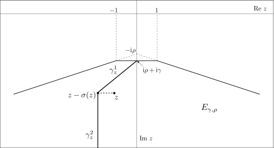
Figure 3: Path $\gamma_{z}$

Given $h$ an analytic function and $z\in E_{\gamma,\rho}$, we introduce the linear operators

$$\Delta^{-1}_{-}(h)(z)=\int_{\gamma_{z}}\frac{h(u)}{\text{e}^{2\pi\text{i}(u-z)}-1}\,du\quad\text{ and }\quad\Delta^{-1}_{+}(h)(z)=\int_{\gamma_{z}}\frac{h(u)}{1-\text{e}^{-2\pi\text{i}(u-z)}}\,du.$$ (82)

Proposition 7.2.

Let $\nu,k\in\mathbb{R}$ and $\gamma>0$. We define the linear operator

$$\Delta^{-1}=\left\{\begin{array}[]{ll}\Delta^{-1}_{-}&\text{if}\;\;\;\;\nu\leq 0\\ \Delta^{-1}_{+}&\text{if}\;\;\;\;\nu>0.\end{array}\right.$$

There exists $\rho_{0}>0$ such that, for any $\rho\geq\rho_{0}$,

1. if $\nu\neq 0$, $\Delta^{-1}:\mathcal{Y}^{\log}_{\nu+1,k,\gamma,\rho}\to\mathcal{Y}^{\log}_{\nu,k,\gamma,\rho}$ is a right inverse of the operator $\Delta$.

2. if $\nu=0$, $\Delta^{-1}:\mathcal{Y}^{\log}_{1,k,\gamma,\rho}\to\mathcal{Y}^{\log}_{0,k+1,\gamma,\rho}$ is a right inverse of the operator $\Delta$.

Moreover in both cases, there exists a positive constant $C$ such that $\|\Delta^{-1}\|\leq C.$

Proof.

Along this proof we will denote by $K$ a generic constant depending only on $\gamma$ and $\nu$. We will skip $\gamma,\rho_{0}$ and $\rho$ from our notation of the Banach spaces and norms.

We fix $\nu\in\mathbb{R}$, $\gamma>0$ fulfilling the hypotheses of Proposition 7.2 and $\rho_{0}\leq\rho$ big enough. Let $h\in\mathcal{Y}_{\nu+1,k}^{\log}$, and we introduce $\varphi=\Delta^{-1}(h)$. Our first observation is that $\varphi$ is an analytic function defined in $E_{\gamma,\rho}$. Indeed, for any $\sigma_{0}>0$ we define the set

$$\Omega_{\sigma_{0}}=\{u\in E_{\gamma,\rho}:u-\sigma_{0}\in E_{\gamma,\rho}\}.$$

We emphasize that $E_{\gamma,\rho}=\cup_{\sigma_{0}>0}\Omega_{\sigma_{0}}$. Moreover we note that, if $z\in\Omega_{\sigma_{0}}$ we can take $\sigma(z)=\sigma_{0}$ in the expression (82) of $\varphi(z)$. Henceforth, in order to deduce that $\varphi$ is an analytic function in $\Omega_{\sigma_{0}}$, we only have to study the convergence of

$$\int_{\gamma_{z}^{2}}\frac{h(u)}{\text{e}^{\mp 2\pi\text{i}(u-z)}-1}\,du$$

To this end, we observe that $|\text{e}^{\mp 2\pi\text{i}(\gamma^{2}_{z}-z)}-1|\geq\left|\text{e}^{\pm t2\pi|\rho+\gamma+\text{Im}z|}-1|\right.$ and that $|h(\gamma_{z}^{2}(t))|\leq C(z)|t|^{-\nu-1}\log^{k}(|t|)$ for some function $C(z)$. Therefore, if $\nu\leq 0$ and $t\in(-\infty,0]$,

$$\frac{|h(\gamma_{z}^{2}(t))|}{|\text{e}^{2\pi\text{i}(\gamma^{2}_{z}-z)}-1|}\leq 2C(z)|t|^{-\nu-1}\log^{k}(|t|)\text{e}^{t2\pi|\rho+\text{Im}z|}$$

and we are done for the case $\nu\leq 0$. The case $\nu>0$ can be done analogously.

Now we are going to check that $\Delta^{-1}$ is a right inverse of the operator $\Delta$. We take into account that, if $z,z+1\in E_{\gamma,\rho}$

$$\Delta\varphi(z)=\mp\int_{\gamma_{z+1}-\gamma_{z}}\frac{h(u)}{\text{e}^{\mp 2\pi\text{i}(u-z)}-1}\,du$$

and therefore, since the only singularity of $\mp h(u)/(\text{e}^{\mp 2\pi\text{i}(u-z)}-1)$ is $u=z$ and it is a simple pole with residue $h(z)/2\pi\text{i}$, we have that both $\varphi_{\pm}$ are solution of $\Delta(\varphi)=h$ defined in the complex domain $E_{\gamma,\rho}$. Here we have proceed exactly as in [FS01].

It only remains to prove that $\varphi=\Delta^{-1}(h)\in\mathcal{Y}_{\nu,k}^{\log}$ provided $h\in\mathcal{Y}_{\nu+1,k}^{\log}$. We restrict ourselves to the complex domain $\widetilde{E}_{\gamma,\rho+\gamma}\subset E_{\gamma,\rho}$ defined by:

$$\widetilde{E}_{\gamma,\rho^{\prime}}=D_{\gamma,\rho^{\prime}}^{{\rm u}}\cap D_{\gamma,\rho^{\prime}}^{{\rm s}}\cap\{z\in\mathbb{C}:\text{Im}z<0\}.$$

We notice that, if the following bounds are proved,

$$|z^{\nu}(\log z)^{-k}\varphi(z)| \leq K\|h\|^{\log}_{\nu+1,k}\;\;\;\;z\in\widetilde{E}_{\gamma,\rho+\gamma} \text{if}\;\;\;\;\nu\neq 0$$ (83)

$$|(\log z)^{-k-1}\varphi(z)| \leq K\|h\|^{\log}_{1,k}\;\;\;\;z\in\widetilde{E}_{\gamma,\rho+\gamma} \text{if}\;\;\;\;\nu=0$$ (84)

the same statement holds for $z\in E_{\gamma,\rho}$. Indeed, assume that bounds (83) and (84) are satisfied and let $z\in E_{\gamma,\rho}\backslash\widetilde{E}_{\gamma,\rho,\gamma}$. We have two cases, $\text{Re}z\leq 0$ and $\text{Re}z>0$. On the one hand, if $\text{Re}\leq 0$, it is clear that $z+1\in\widetilde{E}_{\gamma,\rho+\gamma}$ and that $\varphi(z)=\varphi(z+1)-h(z)$. On the other hand, if $\text{Re}z>0$, $z-1\in\widetilde{E}_{\gamma,\rho+\gamma}$ and consequently $\varphi(z)=\varphi(z-1)+h(z)$. In any case, $|\varphi(z)|\leq|\varphi(z\pm 1)|+|h(z)|$. Here we have used that $\Delta(\varphi)=h$. Therefore, if $\nu\neq 0$, using bound (83), we obtain

$$|\varphi(z)|\leq K\|h\|_{\nu,k}^{\log}\big{(}|z\pm 1|^{-\nu}|\log(z\pm 1)|^{k}\big{)}+|z|^{-\nu-1}|\log z|^{k}\big{)}\leq K\|h\|_{\nu,k}^{\log}|z|^{-\nu}|\log z|^{k}$$

and the result is proved for $\nu\neq 0$. Analogously we check the result for $\nu=0$.

The proof of bounds (83) and (84) is easy but it requires tedious computations which will be omit here. Nevertheless, we point out that for any fixed $z\in\widetilde{E}_{\gamma,\rho+\gamma}$ we can take $\sigma(z)=1/2$ in the definition (7.2) of $\gamma_{z}$. ∎

7.3 Two independent solutions of the linear equation (79)

We recall that $\Theta=\phi^{{\rm u}}-\phi^{{\rm s}}$ satisfies equation (79):

$$\Delta^{2}\Theta=(-Dg(\phi^{{\rm s}})+E)\Theta.$$ (85)

The following lemma states the properties of $E$ we will need. Its proof is completely analogous to the one of bound (74) provided $\phi^{{\rm u}}-\phi^{{\rm s}}\in\mathcal{Y}_{r+2,\gamma,\rho}$.

Lemma 7.3.

Let $\gamma$ and $\rho$ satisfying the conclusions of Proposition 6.2 and $E$ be the function defined in (77). We have that $E\in\mathcal{Y}_{r+6-\ell,\gamma,\rho}$.

As we did in Section 6.1, we split

$$-Dg(\phi^{s})+E=H+M$$

where $H$ was defined in (65), $M\in\mathcal{Y}_{r+2}$, if $n\neq 3$, and $M\in\mathcal{Y}_{r+2,1}^{\log}$, if $n=3$. We rewrite equation (85) as

$$\Delta^{2}(\Theta)-H\cdot\Theta=M\cdot\Theta.$$

A solution of the homogeneous equation $\Delta^{2}(\varphi)=H\cdot\varphi$ is $\eta_{2}(z)=z^{\ell}$. The function

$$\eta_{1}(z)=z^{\ell}\Delta^{-1}\left(\frac{1}{\eta_{2}(z+1)\eta_{2}(z)}\right)\in\mathcal{Y}_{\ell-1}$$

is another solution satisfying $W(\eta_{1},\eta_{2})=1$.

By using these decomposition as well as Proposition 7.2 for the operator $\Delta^{-1}$, we can obtain solutions of the non homogeneous linear equation $\Delta^{2}(\varphi)-H\cdot\varphi=h$.

Lemma 7.4.

For any $\gamma>0$ there exists $\rho_{0}>0$ large enough such that for any $\rho\geq\rho_{0}$, the operator $\mathcal{L}(\varphi)=\Delta^{2}(\varphi)-H\cdot\varphi$ has right inverse defined in $E_{\gamma,\rho}$:

$$\mathcal{L}^{-1}(h)=\eta_{1}\cdot\Delta^{-1}(\eta_{2}\cdot h)-\eta_{2}\cdot\Delta^{-1}(\eta_{1}\cdot h).$$ (86)

There exists $C>0$ such that for any $\alpha\in\mathbb{R}$ and $h\in\mathcal{Y}_{\alpha+2,\gamma,\rho}$, we have:

1. If $\alpha\neq\ell-1$ and $\alpha\neq-\ell$ then $\mathcal{L}^{-1}(h)\in\mathcal{Y}_{\alpha,\gamma,\rho}$ and $\|\mathcal{L}^{-1}(h)\|_{\alpha,\gamma,\rho}\leq C\|h\|_{\alpha+2,\gamma,\rho}$.

2. If either $\alpha=\ell-1$ or $\alpha=-\ell$, $\mathcal{L}^{-1}(h)\in\mathcal{Y}_{\alpha,1,\gamma,\rho}^{\log}$ and $\|\mathcal{L}^{-1}(h)\|_{\alpha,1,\gamma,\rho}^{\log}\leq C\|h\|_{\alpha+2,\gamma,\rho}$.

Next lemma provides a fundamental system of solutions of the linear equation (85).

Lemma 7.5.

Let $\gamma>0$. There exists $\rho_{0}$ large enough such that for any $\rho\geq\rho_{0}$, the equation (85) has two independent solutions, $\hat{\eta}_{1}$ and $\hat{\eta}_{2}$, satisfying

$$\hat{\eta}_{1}(z) =\partial_{z}\phi^{{\rm s}}(z)+\hat{\eta}_{1}^{1}(z),\;\;\;\;\;\hat{\eta}_{1}^{1}\in\mathcal{Y}_{r+3,\gamma,\rho},$$

$$\hat{\eta}_{2}(z) =\frac{z^{\ell}}{rd_{\ell}(2\ell-1)}+\hat{\eta}_{2}^{1}(z),\;\;\;\;\;\hat{\eta}_{2}^{1}\in\mathcal{Y}^{\log}_{\nu,k,\gamma,\rho}$$

with $\nu=\min\{r-\ell,1-\ell\}$, $k=0$ if $n\neq 3$, $k=1$ if $n=3$ and $d_{\ell}$ is defined in (39), .

Proof.

First we look for $\hat{\eta}_{1}$. By construction, $\partial_{z}\phi^{{\rm s}}$ is a solution of the variational equation $\Delta^{2}\varphi=-Dg(\phi^{s})\varphi,$ therefore, the equation that $\hat{\eta}_{1}^{1}$ has to satisfy is

$$\Delta^{2}(\varphi)-H\cdot\varphi=M\cdot\varphi+E\cdot\partial_{z}\phi^{{\rm s}}.$$ (87)

We look for $\hat{\eta}_{1}^{1}$ by means of the fixed point equation

$$\varphi=\mathcal{L}^{-1}(E\cdot\partial_{z}\phi^{{\rm s}})+\mathcal{L}^{-1}(M\cdot\varphi).$$ (88)

We are interested in solutions belonging to $\mathcal{Y}_{r+3}$. It is enough to check that the norm of the linear operator $\mathcal{G}:\mathcal{Y}_{r+3}\to\mathcal{Y}_{r+3}$ defined by $\mathcal{G}(\varphi)=\mathcal{L}^{-1}(M\cdot\varphi)$ is less than one. This fact follows from Lemma 7.4 together with the fact that $E\in\mathcal{Y}_{r+6-\ell}$, $M\in\mathcal{Y}_{r+2}$ if $n\neq 3$ and $M\in\mathcal{Y}_{r+2,1}^{\log}$ if $n=3$. One easily then deduces that

$$\hat{\eta}_{1}^{1}=(\text{Id}-\mathcal{G})^{-1}\big{(}\mathcal{L}^{-1}(E\cdot\partial_{z}\phi^{{\rm s}})\big{)}\in\mathcal{Y}_{r+3}$$ (89)

is a solution of equation (87).

Now we deal with the second solution of the equation (85). We observe that, since $\hat{\eta}_{1}$ is a solution, then the function $\hat{\eta}_{2}=b\cdot\hat{\eta}_{1}$ is also a solution of the linear equation (85) satisfying $W(\hat{\eta}_{1},\hat{\eta}_{2})=1$, if and only if $b$ satisfies

$$\Delta(b)(z)=\frac{1}{\hat{\eta}_{1}(z+1)\hat{\eta}_{1}(z)}.$$

By Proposition 6.2, $\hat{\eta}_{1}=\partial_{z}\phi^{{\rm s}}+\hat{\eta}_{1}^{1}=\partial_{z}\phi_{0}+\partial_{z}\psi^{{\rm s}}+\hat{\eta}_{1}^{1}$ where $\partial_{z}\psi^{{\rm s}},\hat{\eta}_{1}^{1}\in\mathcal{Y}_{r+3}$. Moreover, using the definitions of $d_{\ell},\ell$ in (39) and Corollary 6.3, it is a direct computation to check that $b$ has to satisfy the linear equation

$$\Delta(b)(z)=\frac{z^{2\ell-2}}{r^{2}d_{\ell}^{2}}+S(z)$$

with $S\in\mathcal{Y}_{-2\ell+3}$ if $n=2$, $S\in\mathcal{Y}_{-2\ell+3,1}^{\log}$ if $n=3$ and $S\in\mathcal{Y}_{-2\ell+2+r}$ if $n>3$. We take

$$b_{0}(z)=\frac{z^{2\ell-1}}{r^{2}d_{\ell}^{2}(2\ell-1)}$$

and we note that $r^{2}d_{\ell}^{2}\Delta(b_{0})(z)=z^{2\ell-2}+\mathcal{O}_{-2\ell+3}$. Henceforth, the difference $b_{1}=b-b_{0}$ satisfies an equation of the form

$$\Delta(b_{1})=\tilde{S}(z)$$ (90)

with $\tilde{S}\in\mathcal{Y}_{-2\ell+3}$ if $n=2$, $\tilde{S}\in\mathcal{Y}_{-2\ell+3,1}^{\log}$ if $n=3$ and $\tilde{S}\in\mathcal{Y}_{-2\ell+2+r}$ if $n>3$. Applying Proposition (7.2) one has that equation (90) has a solution $b_{1}$ belonging to $\mathcal{Y}_{-2\ell+2}$ if $n=2$, $\mathcal{Y}_{-2\ell+2,1}^{\log}$ if $n=3$ and $\mathcal{Y}_{-2\ell+1+r}$ if $n>3$ and the result follows. ∎

7.4 A final formula for $\Theta=\phi^{{\rm u}}-\phi^{{\rm s}}$

Since $\Theta$ is a solution of the linear homogenous difference equation (85), the general theory allows us to write it as

$$\Theta(z)=p_{1}(z)\eta_{1}(z)+p_{2}(z)\eta_{2}(z)$$ (91)

with $\eta_{1},\eta_{2}$ two independent solutions of (85) and $p_{1},p_{2}$ $1$-periodic, analytic functions in $E_{\gamma,\rho}$. Moreover, if $W(\eta_{1},\eta_{2})=1$, the functions $p_{1}$ and $p_{2}$ are determined by

$$p_{1}(z)=W(\Theta,\eta_{2})(z),\quad p_{2}(z)=-W(\Theta,\eta_{1})(z).$$ (92)

Lemma 7.6.

Let $\gamma,\rho>0$ and $\eta_{1},\eta_{2}$ two independent solutions of the linear difference equation (85) satisfying that $W(\eta_{1},\eta_{2})=1$ and that $\eta_{1}\in\mathcal{Y}_{r+1}$ and $\eta_{2}\in\mathcal{Y}_{-\ell}$.

Then there exist coefficients $p_{1}^{k},p_{2}^{k}$ (depending on $\eta_{1,2}$) such that

$$\Theta(z)=\eta_{1}(z)\sum_{k<0}p_{1}^{k}\text{e}^{2\pi\text{i}kz}+\eta_{2}(z)\sum_{k<0}p_{2}^{k}\text{e}^{2\pi\text{i}kz}.$$ (93)

Proof.

We first point out that, we already know that $\Theta=\phi^{{\rm u}}-\phi^{{\rm s}}=\psi^{{\rm u}}-\psi^{{\rm s}}\in\mathcal{Y}_{r+2,\gamma,\rho}$ provided that, by Theorem 3.3, $\psi^{{\rm u},{\rm s}}\in\mathcal{X}^{{\rm u},{\rm s}}_{r+2}$. In addition, if $h\in\mathcal{Y}_{\nu,\gamma,\rho}$, then $\Delta(h)\in\mathcal{Y}_{\nu+1,2\gamma,2\rho}$. Indeed, standard arguments can be used to prove that, if $h\in\mathcal{Y}_{\nu,\gamma,\rho}$ then $\partial_{z}h\in\mathcal{Y}_{\nu+1,2\gamma,2\rho}$ (see for instance [Bal06]). Therefore, if $z,z+1\in E_{2\gamma,2\rho}$,

$$|h(z+1)-h(z)|\leq\|\partial_{z}h\|_{\nu+1}\int_{0}^{1}\frac{1}{|z+t|^{\nu+1}}\leq K\|\partial_{z}h\|_{\nu+1}\frac{1}{|z|^{\nu+1}}.$$

Using the above property, that $\Theta\in\mathcal{Y}_{r+2}$ and formula (92) for $p_{1},p_{2}$, one has that $p_{1}\in\mathcal{Y}_{1}$ and $p_{2}\in\mathcal{Y}_{r+4}$. In particular, $p_{1},p_{2}\to 0$ as $\text{Im}z\to-\infty$ and since they are $1$-periodic:

$$p_{1}(z)=\sum_{k<0}p_{1}^{k}\text{e}^{2\pi\text{i}kz},\;\;\;\;\;p_{2}(z)=\sum_{k<0}p_{2}^{k}\text{e}^{2\pi\text{i}kz}$$

ant the lemma is proved. ∎

We recall that the existence of independent solutions of the linear difference equation (85) satisfying the hypotheses of Lemma 7.6 is guaranteed by Lemma 7.5. Henceforth Lemma 7.6 applied to $\hat{\eta}_{1},\hat{\eta}_{2}$ already gives an expression of $\Theta$ which is exponentially small. Among other things, we have proved that there exist $\gamma,\rho>0$ such that

$$|\text{e}^{2\pi\text{i}z}z^{-\ell}(\phi^{{\rm u}}(z)-\phi^{{\rm s}}(z))|\leq K\;\;\;\;\;\;\;z\in E_{\gamma,\rho}.$$ (94)

Nevertheless we have not proved Theorem 3.4 yet. We need to look for more suitable independent solutions of (85) to apply Lemma 7.6.

Corollary 7.7.

Let $\gamma>0$. There exists $\rho_{0}>0$ big enough such that for any $\rho\geq\rho_{0}$, equation (85) has two fundamental solutions of the form

$$\zeta_{1}(z) =\partial_{z}\phi^{{\rm s}}(z)+\zeta_{1}^{1}(z),$$

$$\zeta_{2}(z) =\frac{z^{\ell}}{rd_{\ell}(2\ell-1)}(z)+\zeta_{2}^{1}(z),$$

with with $d_{\ell}$ defined in (39) and $\zeta_{1}^{1}$ satisfying

$$\sup_{z\in E_{\gamma,\rho}}|z^{1-\ell}\text{e}^{2\pi\text{i}z}\zeta_{1}^{1}(z)|<+\infty.$$

In addition, $\zeta_{2}^{1}\in\mathcal{Y}_{r-\ell,\gamma,\rho}$ if $n>3$, $\zeta_{2}^{1}\in\mathcal{Y}_{1-\ell,\gamma,\rho}$ if $n=2$ and $\zeta_{2}^{1}\in\mathcal{Y}_{1-\ell,1,\gamma,\rho}^{\log}$ if $n=3$.

Proof.

As in the proof of Lemma 7.5 we write $\zeta_{1}^{1}=\zeta_{1}-\partial_{z}\phi^{{\rm s}}$. We note that $\zeta_{1}^{1}$ satisfies equation (87):

$$\Delta^{2}(\zeta_{1}^{1})(z)-H(z)\zeta_{1}^{1}(z)=M(z)\zeta_{1}^{1}(z)+E(z)\partial_{z}\phi^{{\rm s}}(z).$$

We write $\zeta(z)=\text{e}^{2\pi\text{i}z}\zeta_{1}^{1}(z)$ and we notice that $\zeta$ has to satisfy the equation

$$\Delta^{2}(\zeta)(z)-H(z)\zeta(z)=M(z)\zeta(z)+\text{e}^{2\pi\text{i}z}E(z)\partial_{z}\phi^{{\rm s}}(z).$$ (95)

We introduce $\varphi_{0}(z)=\text{e}^{2\pi\text{i}z}E(z)\partial_{z}\phi^{{\rm s}}(z)$. We first claim that $\varphi_{0}\in\mathcal{Y}_{3-\ell}$. Indeed, we note that $\partial_{z}\phi^{{\rm s}}\in\mathcal{Y}_{\ell-1}$ and we recall that

$$E(z)=-\int_{0}^{1}(1-\lambda)D^{2}g(\phi^{{\rm s}}+\lambda(\phi^{{\rm u}}-\phi^{{\rm s}}))\,d\lambda\big{(}\phi^{{\rm u}}-\phi^{{\rm s}}\big{)}.$$ (96)

The claim follows from the facts that, by (94), $|z^{-\ell}\text{e}^{2\pi\text{i}z}(\phi^{{\rm u}}-\phi^{{\rm s}})|$ is bounded and moreover $|D^{2}g(\phi^{{\rm s}}+\lambda(\phi^{{\rm u}}-\phi^{{\rm s}}))|\leq K|z|^{\ell-4}$ if $z\in E_{\gamma,\rho}$ (which can be proved as in (74)).

It is clear that, a particular solution $\zeta$ of (95) is given by a solution of

$$\zeta=\mathcal{L}^{-1}(\varphi_{0})+\mathcal{G}(\zeta)$$

being $\mathcal{G}(\zeta)=\mathcal{L}^{-1}(M\cdot\zeta)$.

First we observe that, by Lemma  7.4, the independent term $\mathcal{L}^{-1}(\varphi_{0})\in\mathcal{Y}_{1-\ell}$. Secondly we check that $(\text{Id}-\mathcal{G})$ is invertible in $\mathcal{Y}_{1-\ell}$. Let $\psi\in\mathcal{Y}_{1-\ell}$. Since $M\in\mathcal{Y}_{\frac{r}{2}+2}$ for any $n\geq 2$, we have that $M\cdot\psi\in\mathcal{Y}_{3+\frac{r}{2}-\ell}$ and consequently, by Lemma 7.4, $\mathcal{G}(\psi)\in\mathcal{Y}_{1+\frac{r}{2}-\ell}$ and moreover

$$\|\mathcal{G}(\psi)\|_{1-\ell}\leq\rho^{-r/2}\|\mathcal{G}(\psi)\|_{1+\frac{r}{2}-\ell}\leq\rho_{0}^{-r/2}C\|\psi\|_{1-\ell}\leq\frac{1}{2}\|\psi\|_{1-\ell}.$$

This implies that the norm of the linear operator $\mathcal{G}:\mathcal{Y}_{1-\ell}\to\mathcal{Y}_{1-\ell}$ is less than one and therefore $\text{Id}-\mathcal{G}$ is invertible. To this end, we can write $\zeta$ as

$$\zeta=\big{(}\text{Id}-\mathcal{G}\big{)}^{-1}(\mathcal{L}^{-1}(\varphi_{0}))$$

and we deduce that $\zeta\in\mathcal{Y}_{1-\ell}$ and $\|\zeta\|_{1-\ell}\leq 2\|\mathcal{L}^{-1}(\varphi_{0})\|_{1-\ell}$ which implies the result for $\zeta_{1}$.

The existence and properties of $\zeta_{2}$ follow from the ones for $\hat{\eta}_{2}$ in Lemma 7.5. ∎

References

- [Bal06] I. Baldomá. The inner equation for one and a half degrees of freedom rapidly forced Hamiltonian systems. Nonlinearity, 19(6):1415–1445, 2006.
- [BFGS11] I. Baldomá, E. Fontich, M. Guàrdia, and T. M. Seara. Exponentially small splitting of separatrices beyond melnikov analysis: rigorous results. Preprint avalaible at http://arxiv.org/abs/1201.5152, 2011.
- [Chi79] Boris V. Chirikov. A universal instability of many-dimensional oscillator systems. Phys. Rep., 52(5):264–379, 1979.
- [DG04] Amadeu Delshams and Pere Gutiérrez. Exponentially small spliting for whiskered tori in Hamiltonian systems: continuation of transverse homoclinic orbits. Discrete Contin. Dyn. Syst., 11(4):757–783, 2004.
- [DGJS97] Amadeu Delshams, Vassili Gelfreich, Àngel Jorba, and Tere M. Seara. Exponentially small splitting of separatrices under fast quasiperiodic forcing. Comm. Math. Phys., 189(1):35–71, 1997.
- [DRR98] A. Delshams and R. Ramírez-Ros. Exponentially small splitting of separatrices for perturbed integrable standard-like maps. J. Nonlinear Sci., 8(3):317–352, 1998.
- [DRR99] Amadeu Delshams and Rafael Ramírez-Ros. Singular separatrix splitting and the Melnikov method: an experimental study. Experiment. Math., 8(1):29–48, 1999.
- [DS97] Amadeu Delshams and Tere M. Seara. Splitting of separatrices in Hamiltonian systems with one and a half degrees of freedom. Math. Phys. Electron. J., 3:Paper 4, 40 pp. (electronic), 1997.
- [Fon95] E. Fontich. Rapidly forced planar vector fields and splitting of separatrices. J. Differential Equations, 119(2):310–335, 1995.
- [FS90] E. Fontich and C. Simó. The splitting of separatrices for analytic diffeomorphisms. Ergodic Theory Dynam. Systems, 10(2):295–318, 1990.
- [FS01] Augustin Fruchard and Reinhard Schäfke. Analytic solutions of difference equations with small step size. J. Differ. Equations Appl., 7(5):651–684, 2001. In memory of W. A. Harris, Jr.
- [Gel99] V. G. Gelfreich. A proof of the exponentially small transversality of the separatrices for the standard map. Comm. Math. Phys., 201(1):155–216, 1999.
- [Gel00a] V. G. Gelfreich. Separatrix splitting for a high-frequency perturbation of the pendulum. Russ. J. Math. Phys., 7(1):48–71, 2000.
- [Gel00b] Vassili Gelfreich. Exponentially small splitting of separatrices for area-preserving maps. Chaos Solitons Fractals, 11(1-3):241–243, 2000. Integrability and chaos in discrete systems (Brussels, 1997).
- [Gel00c] Vassili Gelfreich. Splitting of a small separatrix loop near the saddle-center bifurcation in area-preserving maps. Phys. D, 136(3-4):266–279, 2000.
- [GG11] José Pedro Gaivão and Vassili Gelfreich. Splitting of separatrices for the Hamiltonian-Hopf bifurcation with the Swift-Hohenberg equation as an example. Nonlinearity, 24(3):677–698, 2011.
- [GL01] V. Gelfreich and V. F. Lazutkin. Splitting of separatrices: perturbation theory and exponential smallness. Uspekhi Mat. Nauk, 56(3(339)):79–142, 2001.
- [GOS10] Marcel Guardia, Carme Olivé, and Tere M. Seara. Exponentially small splitting for the pendulum: a classical problem revisited. J. Nonlinear Sci., 20(5):595–685, 2010.
- [GS01] V. Gelfreich and D. Sauzin. Borel summation and splitting of separatrices for the Hénon map. Ann. Inst. Fourier (Grenoble), 51(2):513–567, 2001.
- [GS08] Vassili Gelfreich and Carles Simó. High-precision computations of divergent asymptotic series and homoclinic phenomena. Discrete Contin. Dyn. Syst. Ser. B, 10(2-3):511–536, 2008.
- [Laz03] V. F. Lazutkin. Splitting of separatrices for the Chirikov standard map. Zap. Nauchn. Sem. S.-Peterburg. Otdel. Mat. Inst. Steklov. (POMI), 300(Teor. Predst. Din. Sist. Spets. Vyp. 8):25–55, 285, 2003.
- [LMS03] P. Lochak, J.-P. Marco, and D. Sauzin. On the splitting of invariant manifolds in multidimensional near-integrable Hamiltonian systems. Mem. Amer. Math. Soc., 163(775):viii+145, 2003.
- [McM71] E. M. McMillan. A problem in the stability of periodic systems. In W.E. Brittin and Odeabasih, Editors, Topics in Modern Physics: A Tribute to EU Condon, pages 219–244. Colorado Associated University Press, Boulder, CO, 1971.
- [Mel63] V. K. Mel′nikov. On the stability of a center for time-periodic perturbations. Trudy Moskov. Mat. Obšč., 12:3–52, 1963.
- [MSS11a] P. Martín, D. Sauzin, and T. M. Seara. Exponentially small splitting of separatrices in perturbations of the mcmillan map. to appear in DCDS-A, 2011.
- [MSS11b] P. Martín, D. Sauzin, and T. M. Seara. Resurgence of inner solutions for perturbations of the McMillan map. to appear in DCDS-A, 2011.
- [OSS03] C. Olivé, D. Sauzin, and T. M. Seara. Resurgence in a Hamilton-Jacobi equation. Ann. Inst. Fourier (Grenoble), 53(4):1185–1235, 2003.
- [Poi99] H. Poincaré. Les méthodes nouvelles de la mécanique céleste, volume 1, 2, 3. Gauthier-Villars, Paris, 1892–1899.
- [SMH91] Jürgen Scheurle, Jerrold E. Marsden, and Philip Holmes. Exponentially small estimates for separatrix splittings. In Asymptotics beyond all orders (La Jolla, CA, 1991), volume 284 of NATO Adv. Sci. Inst. Ser. B Phys., pages 187–195. Plenum, New York, 1991.
- [Tre97] Dmitry V. Treschev. Splitting of separatrices for a pendulum with rapidly oscillating suspension point. Russian J. Math. Phys., 5(1):63–98 (1998), 1997.