Driven Multifluid MHD Molecular Cloud Turbulence

Abstract

It is believed that turbulence may have a significant impact on star formation and the dynamics and evolution of the molecular clouds in which this occurs. It is also known that non-ideal magnetohydrodynamic effects influence the nature of this turbulence. We present the results of a numerical study of 4-fluid MHD turbulence in which the dynamics of electrons, ions, charged dust grains and neutrals and their interactions are followed. The parameters describing the fluid being simulated are based directly on observations of molecular clouds. We find that the velocity and magnetic field power spectra are strongly influenced by multifluid effects on length-scales at least as large as 0.05 pc. The PDFs of the various species in the system are all found to be close to log-normal, with charged species having a slightly less platykurtic (flattened) distribution than the neutrals. We find that the introduction of multifluid effects does not significantly alter the structure functions of the centroid velocity increment.

1 Introduction

It is generally believed that molecular clouds are turbulent (see the reviews of Mac Low & Klessen 2004; Elmegreen & Scalo 2004). Observationally (e.g. Larson, 1981; Brunt, 2010) this turbulence appears to be highly supersonic with RMS Mach numbers of anything up to 20 or more. It is also thought that the Alfvénic Mach number is not significantly less than one, and may be much greater (e.g. Heyer & Brunt, 2012). The amplitude of this turbulence makes it likely to be an important ingredient in both the dynamics of molecular clouds and the process of star formation (Elmegreen, 1993; Klein et al., 2003) and hence developing an understanding of this phenomenon is of considerable interest.

Many authors have addressed the issue of MHD turbulence in the context of molecular clouds using both the ideal MHD approximation (Mac Low et al., 1998; Mac Low, 1999; Ostriker et al., 2001; Vestuto et al., 2003; Gustaffson et al., 2006; Glover & Mac Low, 2007; Lemaster & Stone, 2008, 2009; Brunt, Federrath, & Price, 2010a; Brunt, Federrath & Price, 2010b; Price, Federrath, & Brunt, 2011) and, more recently, various flavours of non-ideal MHD (Oishi & Mac Low, 2006; Li et al., 2008; Kudoh & Basu, 2008; Downes & O’Sullivan, 2009, 2011). Three dimensional MHD turbulence involves the transfer of energy from an energy injection scale to ever smaller scales until the dissipation length scale of the system is reached. Given that in molecular clouds the lengthscales at which multifluid effects become important are much larger than the viscous lengthscale, it is inevitable that these effects will have an impact on the energy cascade.

When ambipolar diffusion is included in MHD turbulence simulations it has been found that it causes greater temporal variability in the turbulence statistics (Oishi & Mac Low, 2006; Li et al., 2008; Kudoh & Basu, 2008). Although clearly of lesser significance (Wardle & Ng, 1999; Downes & O’Sullivan, 2009, 2011), the Hall effect is capable of inducing topological changes in the magnetic field which are quite distinct to any influence caused by ambipolar diffusion. In particular, it introduces a handedness into the flow which is of particular interest when considering the conversion of kinetic energy into magnetic energy. Researchers working on reconnection and the solar wind have studied the Hall effect in the context of turbulence and found that, although the overall decay rate appears not to be affected, the usual coincidence of the magnetic and velocity fields seen in ideal MHD does not occur at small scales (Matthaeus et al., 2003; Mininni et al., 2006; Servidio et al., 2007).

Downes & O’Sullivan (2009, hereafter Paper I) performed simulations of decaying, non-ideal MHD, molecular cloud turbulence incorporating parallel resistivity, the Hall effect and ambipolar diffusion. They found that the Hall effect has surprisingly little impact on the behaviour of the turbulence: it does not affect the energy decay at all and has very limited impact on the power spectra of any of the dynamical variables, with the exception of the magnetic field at very short length-scales. Downes & O’Sullivan (2011, hereafter Paper II) extended the results of Paper I to properly multifluid MHD turbulent decay. A system of three fluids, 1 neutral and two charged species, was simulated and, intriguingly, it appears that for the chosen system a full multifluid simulation is unnecessary and simple non-ideal MHD with temporally and spatially constant resistivities can give quite reliable results.

In this paper we use the HYDRA code (O’Sullivan & Downes, 2006, 2007) to investigate driven, isothermal, multifluid MHD turbulence in a system consisting of 4 fluids (1 neutral and 3 charged). The aim of this work is to determine the influence of multifluid effects on the behaviour of driven turbulence in molecular clouds. An added benefit of our properly multifluid approach is that we can self-consistently deduce the behaviour of the charged species and, in principle, make links with observations such as those of Li & Houde (2008).

The structure of this paper is as follows: in section 2 we outline the equations and numerical method; in section 3 we specify our parameters, initial conditions and how we drive the turbulence in our simulations; section 5 contains the results of a resolution study demonstrating that the results we present are reasonably well converged; section 6 contains the results and analysis of our simulations and finally we draw conclusions from our work in section 7. We note here that we omit a discussion of the differences in line widths between the charged and the neutral species. The results associated with these differences require detailed discussion in their own right and are the subject of a forthcoming paper.

2 The model

Molecular clouds are, to a great extent, weakly ionised systems. This allows us to make several simplifying assumptions, as follows:

• The bulk flow velocity is the neutral velocity

• The majority of collisions experienced by each charged species occur with neutrals

• The charged species’ inertia is unimportant

• The charged species’ pressure gradient is unimportant

Making these assumptions allows us to derive a relationship between the electric field and the current density. This generalised Ohm’s law (e.g. Falle, 2003; Ciolek & Roberge, 2002) allows us to avoid having to calculate the electric field explicitly from the charge distribution.

2.1 Equations

Once we have our generalised Ohm’s law, the system of equations for our weakly ionised flow is as follows (e.g. Falle, 2003)

$$\frac{\partial\rho_{i}}{\partial t}+\mbox{\boldmath$\nabla$}\cdot\left(\rho_{i}\mbox{\boldmath$u$}_{i}\right) = 0\mbox{, ($1\leq i\leq N$), }$$ (1)

$$\frac{\partial\rho_{1}\mbox{\boldmath$u$}_{1}}{\partial t}+\mathbf{\nabla}\cdot\left(\rho\mbox{\boldmath$u$}_{1}\mbox{\boldmath$u$}_{1}+a^{2}\rho\mbox{\boldmath$\mathsf{I}$}\right) = \mbox{\boldmath$J$}\times\mbox{\boldmath$B$},$$ (2)

$$\frac{\partial\mbox{\boldmath$B$}}{\partial t}+\mathbf{\nabla}\cdot(\mbox{\boldmath$u$}_{1}\mbox{\boldmath$B$}-\mbox{\boldmath$B$}\mbox{\boldmath$u$}_{1}) = \mathbf{\nabla}\times\left\{r_{0}\frac{(\mathbf{J}\cdot\mathbf{B})\mathbf{B}}{B^{2}}+r_{1}\frac{\mathbf{J}\times\mathbf{B}}{B}+r_{2}\frac{\mathbf{B}\times(\mathbf{J}\times\mathbf{B})}{B^{2}}\right\},$$ (3)

$$\alpha_{i}\rho_{i}\left(\mbox{\boldmath$E$}^{\prime}+\mbox{\boldmath$u$}_{i}\times\mbox{\boldmath$B$}\right) = -\rho_{i}\rho_{1}K_{i\,1}(\mbox{\boldmath$u$}_{1}-\mbox{\boldmath$u$}_{i})\mbox{, $2\leq i\leq N$, }$$ (4)

$$\mathbf{\nabla}\cdot\mbox{\boldmath$B$} = 0,$$ (5)

$$\mathbf{\nabla}\times\mbox{\boldmath$B$} = \mbox{\boldmath$J$},$$ (6)

$$\sum_{i=2}^{N}\alpha_{i}\rho_{i} = 0.$$ (7)

where $i$ denotes the species (with $i=1$ denoting the neutral species), $\rho_{i}$, $\mbox{\boldmath$u$}_{i}$, $a$, $B$, $\mathsf{I}$, $J$ and $\mbox{\boldmath$E$}^{\prime}$ are the mass density of species $i$, the velocity of species $i$, the isothermal sound speed, the magnetic field, the identity matrix, the current density and the electric field in the neutral rest frame, respectively. The parameters $\alpha_{i}$ and $K_{i1}$ are the charge-to-mass ratios and the collision coefficient with the neutrals for species $i$.

These equations describe conservation of mass for all species, the neutral momentum equation, the induction equation, force balance for the charged species, the absence of magnetic monopoles, Faraday’s Law and charge neutrality. In the work presented here we set $N=4$.

The electric field in the frame of the fluid, $\mbox{\boldmath$E$}^{\prime}$, is calculated from the generalised Ohm’s law for weakly ionised fluids (e.g. Falle 2003; O’Sullivan & Downes 2006) and is given by

$$\mbox{\boldmath$E$}^{\prime}=\mbox{\boldmath$E$}_{\rm 0}+\mbox{\boldmath$E$}_{\rm 1}+\mbox{\boldmath$E$}_{\rm 2},$$ (8)

where

$$\mbox{\boldmath$E$}_{\rm 0} = (\mbox{\boldmath$J$}\cdot\mbox{\boldmath$a$}_{\rm 0})\mbox{\boldmath$a$}_{\rm 0},$$ (9)

$$\mbox{\boldmath$E$}_{\rm 1} = \mbox{\boldmath$J$}\times\mbox{\boldmath$a$}_{\rm 1},$$ (10)

$$\mbox{\boldmath$E$}_{\rm 2} = -(\mbox{\boldmath$J$}\times\mbox{\boldmath$a$}_{\rm 2})\times\mbox{\boldmath$a$}_{\rm 2},$$ (11)

using the definitions $\mbox{\boldmath$a$}_{\rm 0}\equiv f_{\rm 0}\mbox{\boldmath$B$}$, $\mbox{\boldmath$a$}_{\rm 1}\equiv f_{\rm 1}\mbox{\boldmath$B$}$, $\mbox{\boldmath$a$}_{\rm 2}\equiv f_{\rm 2}\mbox{\boldmath$B$}$, where $f_{\rm 0}\equiv\sqrt{r_{\rm 0}}/B$, $f_{\rm 1}\equiv r_{\rm 1}/B$, $f_{\rm 2}\equiv\sqrt{r_{\rm 2}}/B$. $r_{\rm 0}$, $r_{\rm 1}$ and $r_{\rm 2}$ are the parallel, Hall and ambipolar resistivities respectively and are given by

$$r_{\rm 0} = \frac{1}{\sigma_{\rm 0}},$$ (12)

$$r_{\rm 1} = \frac{\sigma_{\rm 1}}{\sigma_{\rm 1}^{2}+\sigma_{\rm 2}^{2}},$$ (13)

$$r_{\rm 2} = \frac{\sigma_{\rm 2}}{\sigma_{\rm 1}^{2}+\sigma_{\rm 2}^{2}},$$ (14)

with the conductivities given by

$$\sigma_{\rm 0} = \frac{1}{B}\sum_{i=2}^{N}\alpha_{i}\rho_{i}\beta_{i},$$ (15)

$$\sigma_{\rm 1} = \frac{1}{B}\sum_{i=2}^{N}\frac{\alpha_{i}\rho_{i}}{1+\beta_{i}^{2}},$$ (16)

$$\sigma_{\rm 2} = \frac{1}{B}\sum_{i=2}^{N}\frac{\alpha_{i}\rho_{i}\beta_{i}}{1+\beta_{i}^{2}},$$ (17)

where $\beta_{i}$ is the Hall parameter for species $i$ and is given by

$$\beta_{i}=\frac{\alpha_{i}B}{K_{1\,i}\rho_{1}}.$$ (18)

2.2 Numerical method

Equations (1) – (7) are a nonlinear system of PDEs and, in general, must be tackled using simulations. With modern techniques the system is relatively straightforward, with the exception of dealing with the right-hand side of equation (3). The method used by HYDRA to integrate these equations has been elucidated previously in the literature (e.g. O’Sullivan & Downes, 2006, 2007) so we only give a brief recapitulation of this here and refer the reader to these papers for a more in-depth discussion.

The system is solved using an operator-split approach with three operators:

• The equations governing the neutrals are solved using a standard second order, shock capturing Godunov scheme. The induction equation is also solved as part of this operator, but without incorporation of the non-ideal effects. The divergence of the magnetic field is controlled using the method of Dedner et al. (2002).

• The magnetic diffusion terms are evaluated and applied using the super-time-stepping method (for the ambipolar and parallel resistivity terms) and the Hall Diffusion Scheme (for the Hall term).

• The velocities of the charged species are determined from equation (4) and the distribution of their densities are updated using a second order upwind scheme.

The whole system of operators is stepped forward in time using Strang operator splitting in order to ensure second order accuracy in time.

Since molecular cloud material has very low kinematic viscosity (e.g. Jones & Downes, 2012), flows, these systems have a high Prandtl number and thus we can consider them to be effectively inviscid. As with all higher-order schemes, our simulations incorporate artificial viscosity which smears discontinuities over around 3 – 5 grid zones. This artificial viscosity length scale is much less than that over which the multifluid effects act (see, for example, figure 2) and thus our multifluid effects dominate at all scales above around 3 – 5 grid zones. Formally, the Prandtl number of the highest resolution simulations in this work is around 15.

The method is explicit and scales extremely well on massively parallel systems, displaying strong scaling from 8192 up to 294,912 cores with 73% efficiency on the JUGENE BlueGene/P system in Jülich, Germany.

3 Numerical set-up

We run our turbulence simulation in a cube of side 0.2 pc with periodic boundary conditions on all faces. The density is initially uniform and has the value of $10^{4}$ cm^-3, assuming that the average neutral particle has a mass of 2.33 $m_{\rm p}$ (where $m_{\rm p}$ is the mass of the proton). The magnetic field is also initially uniform of strength 20 $\mu$G respectively. The (isothermal) sound-speed is chosen to be $1.88\times 10^{4}$ cm s^-1 or, equivalently, the temperature is 10 K. The four fluids in the system are initially at rest. These parameters were chosen to be representative of molecular clouds on scales of 0.2 pc and are based on the data in Table 1 of Crutcher (1999). The grid used is uniform and made up of $N_{x}\times N_{y}\times N_{z}$ grid points with $N_{x}=N_{y}=N_{z}=N_{\rm g}$. We emphasise here that this work is directed at understanding the nature of multifluid MHD turbulence. A physical system with the properties just described will have a mass just below the Jeans mass and so may well be subject to dynamically important self-gravity. However, it seems reasonable that the optimal way of approaching understanding the behaviour of molecular clouds is to first attempt to understand the turbulence, and then to introduce self-gravity. Introducing all the physical effects at once runs the risk of producing results which, while possibly valid, are very difficult to interpret.

The properties of the charged species are based on the data in Wardle & Ng (1999). We make the approximation that the dust density is 1% that of the neutrals. The metal ions are assumed to be singly ionised and to have an average mass of 24 $m_{\rm p}$ and a mass density of $1.27\times 10^{-25}$g cm^-3. The electron density is then chosen to ensure local charge neutrality. This set-up results in an ionisation fraction of approximately $3\times 10^{-7}$ and the system is therefore clearly weakly ionised.

In order to drive turbulence we add velocity increments to the neutral velocity at each time-step. The incremental velocity field, $\delta\mbox{\boldmath$u$}$, is defined in a manner similar to Lemaster & Stone (2009). Each component of $\delta\mbox{\boldmath$u$}$ is generated from a set of waves with wave numbers, $k=|\mbox{\boldmath$k$}|$, $3\leq k\leq 4$. The amplitudes of these waves are drawn from a Gaussian random distribution with mean 1.0 and deviation 0.33 while the phases of the waves are drawn from a uniform distribution between 0 and $2\pi$. The waves are chosen such that the forcing is solenoidal. It is known that the precise nature of the forcing will influence the turbulence statistics (e.g. Federrath et al., 2011). In this paper we focus on gaining some insight into the influences of multifluid effects on turbulence and leave a study of multifluid MHD turbulence under differing driving to a later date.

Finally, to ensure a constant energy injection rate and zero net momentum injection, a quadratic equation must be solved to normalise $\delta\mbox{\boldmath$u$}$. The resulting normalised incremental velocity field is then added on to the neutral velocity field. The rate of injection of energy is the same for all simulations in this work and is given by $\frac{\dot{E}}{\rho_{0}L^{2}a^{3}}=200$ where $\rho_{0}$ is the initial (uniform) density, $L$ is the length of side of the computational domain and $a$ is the (isothermal) sound speed. In our simulations this energy injection rate yields steady state turbulence with an RMS Mach number of around 4.5 and an Alfvénic Mach number of between 3 and 3.5.

Table 1 contains the definition of the nomenclature of the various simulations used in this work.

Name	Resolution ($N_{\rm g}$)	Physics
mf-64	64	Multifluid MHD
mf-128	128	Multifluid MHD
mf-256	256	Multifluid MHD
mhd-256	256	Ideal MHD

Table 1: Definition of the nomenclature used to refer to the various simulations presented in this work.

4 Analysis

There are two different, but related, aspects to analysing the multifluid simulations presented here. The first is associated with understanding the dynamics of the bulk flow, while the second is focused on the interplay, and differences, between the behaviour of the various species in the simulation. In both cases, however, we can use analysis techniques which are broadly similar.

4.1 Power spectra

One of the most popular things to do when faced with a set of results from turbulence simulations is to take power spectra. These spectra give information on the relative size of structures formed by turbulence in the system. In incompressible hydrodynamic turbulence this is easily visualised as, for example, the energy residing in vortices of differing sizes. Standard Kolmogorov theory predicts that, in the absence of driving or dissipation, the power spectrum will take on a power-law form, and the exponent of this power law can be predicted in a relatively straightforward manner. For incompressible MHD turbulence the situation is a little more complicated, while for compressible MHD turbulence it becomes more complicated again. However, the power spectra of the fluid variables still provide useful physical insight into the type of turbulence occurring.

The power spectra presented here are calculated by taking a 3D Fourier transform of the relevant fluid variable. The total power residing in a spherical shell of inner radius $k$ and outer radius $k+dk$ is then calculated and it is this quantity which we present in our power spectra. When discussing wave numbers we use the notation $k\equiv\frac{L}{2\pi}\tilde{k}$ where $\tilde{k}$ is the usual wave number. Then $k$ is the number of waves which fit into the computational domain for that value of $\tilde{k}$. In calculating the power spectra we use $dk=1$. The power spectra are taken for different times and the results presented here are the time-averaged spectra. For all simulations the spectra are averaged over $t=[0.2,0.52]$ sound crossing times, or $[0.9,2.34]$ flow crossing times.

4.2 The centroid velocity

The statistics of the centroid velocity are, in principle at least, an observable quantity and are therefore of some physical interest (e.g. Hily-Blant, Falgarone, & Pety, 2008; Federrath et al., 2010). Suppose we orient our simulation cube such that the $z$ direction is along the line of sight, leaving the $x$ and $y$ directions in the plane of the sky. The centroid velocity is then defined as

$$C(x,y)=\frac{\int\rho(x,y,z)v_{z}(x,y,z)\,dz}{\int\rho(x,y,z)\,dz}$$ (19)

The density weighting used here to calculate the average line-of-sight velocity can be thought of as some approximation to what happens when observations are made and the average line-of-sight velocity is actually the emission-weighted average.

Having defined our centroid velocity we can then consider the centroid velocity increment, defined by

$$\delta C_{l}(\mathbf{r})=\left<C(\mathbf{r})-C(\mathbf{r}+\mathbf{l})\right>$$ (20)

where $\mathbf{r}=(x,y)$ and $\mathbf{l}$ is a vector of length $l$ and the average is calculated over all possible directions of $\mathbf{l}$ in the $(x,y)$ plane.

Finally we introduce the associated centroid velocity increment structure functions, defined by

$${\rm CVISF}_{p}(l)\equiv<|\delta C_{l}(\mathbf{r})|^{p}>_{\mathbf{r}}$$ (21)

where $p$ is the order of the structure function. These quantities are discussed in Sect. 4.2.

5 Resolution study

We performed identical simulations with differing resolutions in order to determine what aspects of the results from our highest resolution simulation are well converged. The resolutions used were $N_{\rm g}=64$, 128 and 256 (see Sect. 3). Table 2 contains a summary of our results from the resolution study.

Simulation	$M_{\rm s}$	$M_{\rm A}$	Velocity power spectrum
mf-64	4.38	2.77	$-2.54\pm 0.26$
mf-128	4.47	3.01	$-2.40\pm 0.23$
mf-256	4.48	3.07	$-2.40\pm 0.05$
mhd-256	4.41	3.17	$-1.81\pm 0.05$

Table 2: The time-averaged RMS sonic Mach and Alfvén numbers and the slope of the velocity power spectra for the simulations presented in this work. The velocity power spectrum is fitted over the range $[4:N_{\rm g}/16]$ in each case with the exception of mf-64 where the range is $[4:8]$. $N_{\rm g}$ is the number of grid zones along a side of our cube. The error quoted is the formal error from the least squares fitting.

Figure 1 contains plots of the RMS Mach number as a function of time for each of the simulations in our resolution study. It is clear that after an initial period of time during which the turbulence is building up, each simulation reaches a quasi-steady state with an RMS turbulent Mach number of between 4.3 and 4.5.

The highest Mach number reached occurs, perhaps unsurprisingly, in the $256^{3}$ simulation. However, after this initial maximum, the average Mach number in each case is rather similar, bearing in mind the stochastic nature of the simulations, with the $128^{3}$ and the $256^{3}$ simulations giving results within about $0.2$% of each other. Simulation mf-64 does have a somewhat lower RMS Mach number (see Table 2), indicating that at this low resolution the global energy dissipation rate is significantly influenced by numerical viscosity. However, the similarity of the Mach numbers for mf-128 and mf-256 indicate that the global energy dissipation rate is well captured with a resolution of $256^{3}$.

Figure 1: Plot of the RMS Mach number as a function of time for each of the simulations in the resolution study.

Figure 2: Plot of the time-averaged, compensated neutral velocity power spectrum for each of the simulations in the resolution study. See also Table 2. The spectra are compensated by $k^{2.2}$.

Another measure of whether or not turbulence simulations have converged is the slope of the power spectrum of the velocity. Figure 2 contains plots of the compensated power spectrum of the neutral velocity for each of the three simulations in the resolution study. While we generally expect this power spectrum to behave as a power law, there will be some value of $k$ at which the spectrum will steepen due to numerical dissipation effects. In order to get a picture of the range of $k$ over which we can trust our results, we have fitted the power spectrum with a power-law over various different ranges. The driving occurs at $3\leq k\leq 4$ and we find that between $k=4$ and $k\approx\frac{N_{\rm g}}{16}$ ($N_{\rm g}$ being the number of grid zones along a side of our cube) our slopes are very similar, keeping in mind the formal errors, across all resolutions (see Table 2). These results give support to the idea that these simulations have resolved the turbulent cascade, at least up to a value of $k$ of around $\frac{N_{\rm g}}{16}$ zones. Even so, when interpreting the results in a quantitative fashion, the size of the formal errors must be kept in mind and the best way to reduce these is through using higher resolution simulations. The results of Federrath et al. (2010) suggest that caution must be used when interpreting power spectra at high $k$. In their particular work where FLASH3 was used they found the power spectra to be susceptible to numerical dissipation below length scales of about 30 grid zones. Our resolution study here demonstrates that the equivalent length scale, for velocity power spectra, for HYDRA is about 10 – 15 grid zones.

6 Results

Following the results of our resolution study we are reasonably confident that our $N_{\rm g}=256$ simulation is well enough resolved to draw some useful physical conclusions about the behaviour of driven, multifluid MHD turbulence.

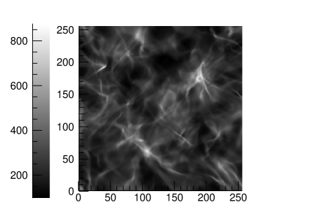
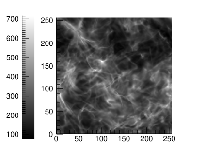
Figure 3: Distribution of the column density for mf-256 (upper panel) and mhd-256 (lower panel) at time $t=0.5$ $t_{\rm c}$, assuming the line of sight is along the $z$ axis. The units on the $x$ and $y$ axes are grid zones and the density is in units of $10^{4}$ cm^-3.

Figure 3 contains plots of the (neutral) column density for the multifluid and ideal MHD simulations. It is apparent that there is somewhat more small scale structure in mhd-256 than in mf-256. The maxima and minima of the column density are broadly similar in each case.

6.1 Energy dissipation

Figure 4 contains plots of the behaviour of the mean, mass-weighted RMS Mach and Alfvén numbers (see Lemaster & Stone, 2009; Downes & O’Sullivan, 2011). It is clear that the Mach number reached in each case is very similar. Table 2 demonstrates this in quantitative terms with the difference in time-averaged RMS Mach number after $t=0.2$ $t_{\rm c}$ being around than 1.6%. Therefore, at these length scales and with this numerical resolution, we do not detect any difference in the energy dissipation rate due to multifluid effects. Note that the RMS Mach number is actually a simple measure of the RMS velocity on the computational grid as the simulations are isothermal. On the other hand, the RMS Alfvén number is a more complicated quantity, given that the Alfvén speed is a spatially and temporally varying quantity. It is clear that the difference in the Alfvén numbers between mhd-256 and mf-256 are rather small, with a difference of only around 3%. This is quite interesting, given that ambipolar diffusion does diffuse magnetic energy and hence would be expected to lower the Alfvén speed generally. Hence, taken together, the similarities between mf-256 and mhd-256 with respect to their Mach and Alfvén numbers indicates that the Alfvén speed is not, in fact, lowered significantly on a global scale by multifluid effects.

The results presented in Papers I and II imply that the energy dissipation rate is higher in multifluid MHD systems. We would expect, then, that the mean Mach number would be lower in mf-256 than in mhd-256. However, it is clear from Table 2 that this is not the case. If, instead of the time-averaged mass-weighted RMS Mach number, we calculate the time-averaged RMS Mach number without mass-weighting, we find that the RMS Mach numbers are 4.18 and 4.10 for mhd-256 and mf-256 respectively. This is a little more in line with what we would naively expect although, on the face of it, it still does not indicate significantly increased energy dissipation due to multifluid effects. When considering this issue, it is significant that the main contribution to the RMS Mach numbers in each of mhd-256 and mf-256 comes from large scale motions - i.e. motions close to the driving scale. Since the multifluid effects operate at relatively short length scales it, perhaps, is not too surprising that the RMS Mach number is not effected much by the inclusion of these effects. When reconciling this result with those of Papers I and II it is worth recalling that these latter results were calculated for decaying turbulence. As turbulence decays energy initially injected at large scales cascades to ever smaller scales. Thus decaying multifluid turbulence will exhibit a faster Mach number decay as, in contrast to driven turbulence, the main contribution to the measured Mach number will come from ever smaller scales, and thus be more influenced by multifluid effects.

There is a further effect to take into account. Closer examination of the data from mf-256 and mhd-256 reveals that, while the kinetic energies in each simulation are very similar, the magnetic energy in the multifluid simulation is much decreased (see Figure 5). This reduction in the magnetic energy is due to the presence of ambipolar diffusion and shows that the multifluid effects do have a significant impact on the energetics of the system. The fact that the RMS Mach number is not strongly influenced by multifluid effects is partly a reflection of the fact that the energy in the system is dominated by kinetic energy. Some of this kinetic energy is converted into magnetic energy but, even in mhd-256, this is a relatively small proportion: on average the magnetic energy is around 40% of the kinetic energy. The fact that this converted energy is then lost faster in mf-256 has relatively little impact on the large reservoir of kinetic energy, and therefore has a minor influence on the RMS Mach number. On a side note, it is interesting to note the results of Federrath et al. (2011) in which studies of dynamo action in MHD simulations of turbulence. These authors found that, as might be expected, solenoidally forced turbulence induces stronger dynamo action. The relevant saturation levels for the ratio of magnetic to kinetic energy from that study are around 0.03, considerably smaller than the results presented here. However, the significant differences in terms of initial conditions between this latter study and the one presented here make it difficult to draw any firm conclusions about the origins of the differences between the results.

In the case of decaying turbulence, the magnetic energy becomes approximately equal to the kinetic energy as the decay process continues (see Figure 6 of Paper I) and hence the multifluid effects can have a more significant impact on the overall energetics of the system, resulting in a faster decay rate.

Figure 4: Plot of the RMS Mach and Alfvén numbers as functions of time for mf-256 and mhd-256.

Figure 5: Plot of the total perturbed magnetic energy in the computational domain as a function of time for mf-256 and mhd-256.

6.2 Power spectra

We now turn to the power spectra of the various quantities of interest in these simulations. The nature of these spectra will give us some idea of the influence of the multifluid effects on the turbulence. As noted previously, we time-average all power spectra discussed here over the time-interval $[0.2\,t_{\rm c}:0.52\,t_{\rm c}]$. Table 3 contains the exponents of the power spectra, fitted assuming the spectrum goes as $k^{\alpha}$. The fitting is carried out over the same range as that in Table 2 and so we are reasonably confident that the exponents we find are not significantly influenced by numerical resolution effects.

Table 3: Exponents of the power spectra of the various variables in the mf-256 and mhd-256 simulations. The spectra were fitted as power laws in the range $4\leq k\leq\frac{N_{\rm g}}{16}$.

	mhd-256	mf-256
		Neutrals	Electrons	Dust	Ions
Density	-0.60	-0.83	-0.99	-1.11	-0.99
Velocity	-1.81	-2.40	-2.17	-2.19	-2.17
$\mathbf{B}$-field	-1.73	-2.26

6.2.1 Velocity power spectra

The compensated velocity power spectra for the neutrals in mf-256 and the bulk fluid in mhd-256 are shown in figure 6. The power is compensated with $k^{1.8}$ which is the measured exponent of the velocity spectrum of mhd-256 (see Table 3). It is clear, as indicated also in Table 3, that the multifluid effects modify the velocity power spectra of the neutrals significantly, even on rather large length scales.

Figure 6: Time-averaged compensated, spherically integrated velocity power spectra for the neutrals in mf-256 and the bulk flow in mhd-256. The spectra are compensated with $k^{1.8}$.

Figure 7 contains plots of the spherically integrated, compensated velocity power spectra for the neutrals, electrons and dust in mf-256. We have omitted a plot of the spectrum for the ions as it is virtually identical to that for the electrons. It is clear that the velocity power spectra for the neutrals and charged species do differ to some extent on these length scales (i.e. all scales up to 0.05 pc). The spectrum for the charged species is somewhat harder than the neutrals. This is in line with what would be expected in a multifluid system affected by ambipolar diffusion: as ambipolar diffusion becomes more important the neutrals behave more like a hydrodynamic system which characteristically has a softer velocity power spectrum than an MHD system. The charged species remain more affected by the magnetic field and therefore retain more strongly the characteristics of MHD turbulence. Another way of looking at this is to observe that, from the data in Table 3, the power spectra of the velocity for the charged species have exponents which lie between that for the neutrals and that for ideal MHD. Again, this is what would be expected given the more direct link between the behaviour of the charged species and that of the magnetic field. At very high $k$ there is a slight difference between the dust and electron power spectrum, almost certainly due to the Hall term in the induction equation. However, we should refrain from attaching quantitative physical significance to this as the length scales involved at these values of $k$ are too short to be reliably resolved in the simulation.

Figure 7: Time-averaged, compensated, spherically integrated velocity power spectra for the neutrals, electrons and dust in mf-256. The spectrum for ions is virtually identical to that for electrons and is omitted.

6.2.2 Density power spectra

Density power spectra, while not as dynamically relevant in supersonic turbulence as velocity power spectra, nonetheless provide an insight into the size of structures formed by the turbulence (e.g. Ossenkopf & Mac Low, 2002). This can also be investigated in a different way using the probability density function (PDF) of the density which we discuss later (Sect. 6.3). Figure 8 contains plots of the time-averaged (neutral) density power spectra for mf-256 and mhd-256.

Figure 8: Plots of the time-averaged power spectra for the neutral density in mf-256 and the density in mhd-256. The spectra are compensated using $k^{0.6}$ (see Table 3).

There is less power in the bulk density of mf-256 than mhd-256 for all $k\geq 10$ as one might expect, given the similarity between the multifluid effects and viscosity and also given the behaviour of the velocity power spectra. Interestingly, there is marginally less power in mhd-256 than mf-256 at $k<10$. This difference is rather small and is likely to be due to diffusive effects causing an inverse cascade, as would be expected since they smooth out small scale structures into larger scale ones.

While there is somewhat less power in the density variations in mf-256 than mhd-256, there are striking differences between the power in the density variations of the neutral and charged species in mf-256 (see Figure 9). Hence we have a situation where the neutral power spectrum is more qualitatively similar to that obtained from ideal MHD, while the charged species (which are more directly influenced by the magnetic field) have significantly less power at virtually all length scales. A careful comparison of figure 10 and the upper panel of figure 3 reveals that, even by eye, there is less structure in, for example, the dust distribution than the neutral distribution.

The inclusion of multifluid effects leads to the introduction of terms in the induction equation which are diffusive so it is not a surprise that there is less structure in a multifluid MHD system than an ideal MHD one. It is also, perhaps, not surprising that this lack of structure is particularly marked in the charged species which are more directly affected by the dynamics of the magnetic field.

Figure 9: Plots of the the time-averaged, normalised power spectra of the density for all species in mf-256. The spectra are normalised and compensated by $k^{0.6}$ for ease of comparison (see Table 3). The power spectrum for the ions is not plotted as it is identical to that for electrons.

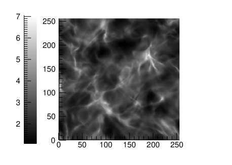
Figure 10: Distribution of the column density for the dust in our mf-256 simulation at time $t=0.5$ $t_{\rm c}$, assuming the line of sight is along the $z$ axis. The units on the $x$ and $y$ axes are grid zones and the density is in units normalised by the initial neutral density. Comparison with the upper panel in figure 3 indicates there is less small-scale structure in the dust distribution.

6.2.3 Magnetic field power spectra

We now turn our attention to the power spectra of the magnetic fields in each simulation (see Fig. 11). In keeping with the velocity and density power spectra (Figs. 8 and 6), there is less structure on all scales, even at the driving scale, in the multifluid system than in the ideal MHD system. This is due to the presence of ambipolar diffusion which, being a standard diffusion term in the induction equation, will smear out any small scale structure. This result implies that multifluid effects can have an impact on the nature of molecular cloud turbulence even at fairly large length scales - much larger than those inferred from, for example, the observations of Li et al. (2008, 2010). We address this apparent contradiction in a forthcoming paper.

It is worth noting again that the Hall effect is present in this system, albeit at a much lower level than ambipolar diffusion. As in Paper I and Paper II we find little evidence of the Hall effect at length scales which are numerically resolved in our power spectra. At very short length-scales ($k\geq 100$) we can see an upturn in the power spectrum for the magnetic field and the charged species (Figure 7) and this is almost certainly the influence of the Hall effect where, as expected, we see a decoupling at short length scales between the neutrals and the charged species, as well as the magnetic field. The phenomenon of the Hall effect having somewhat less impact than would be expected was also discussed in Jones & Downes (2012) who deduced that the presence of ambipolar diffusion can effectively short circuit the Hall current, thereby inhibiting the Hall effect even in systems with significant Hall resistivity.

Figure 11: Time-averaged, compensated, spherically integrated magnetic field power spectra for mf-256 and mhd-256. Each power spectrum is compensated with $k^{7/4}$.

6.3 Probability Density Functions

Probability density functions (PDFs), in particular of the mass density, are particularly interesting when considering the influence molecular cloud turbulence may have on star formation. It has long been known that isothermal, supersonic turbulence results in a log-normal PDF of the density (e.g. Vázquez-Semadeni, 1994; Passot & Vázquez-Semadeni, 1998). This is due simply to the fact that the density of a particular fluid element is a product of its initial value and all of the enhancements at each of the shocks it has encountered. Since the shock strengths are randomly distributed, the density is thus the result of a product of random variables and hence its distribution is log-normal. Several researchers have shown that the addition of gravity to the physics of the system adds a long, high mass tail to the PDF (e.g. Klessen, 2000; Dib & Burkert, 2005), presumably due to the influence of gravity which will produce accumulations of mass in small regions which would not be expected to happen to the same extent with isothermal turbulence. This would lead to a positive skewness of the density distribution or, to say it another way, the distribution being skewed right.

Figure 12 contains plots of the PDF of the logarithm of the density of the bulk flow of mhd-256 and mf-256. Table 4 details the standard deviation, skewness and excess kurtosis of the distributions of all of the densities in our simulations. Clearly all of the densities in each of mf-256 and mhd-256 have very close to a log-normal distribution. The logarithm of the bulk mass density is very slightly platykurtic in both mf-256 and mhd-256, while the distributions of the charged densities are a mix of leptokurtic and platykurtic. However, these differences in the kurtosis are rather minor. The skewness of these distributions is also small, indicating again how close to log-normal the PDF of the density of the bulk flow is.

Examining Figure 13 and Table 4 we see that the charged species are slightly less platykurtic (flattened) than the neutrals in mf-256. We can understand this as follows: the magnetic field has, of course, a pressure associated with it which will resist both compression and rarefaction. Since the charged species are, by definition, more closely tied to the magnetic field than the neutrals we expect that the neutrals will undergo more severe compressions and rarefactions than the charged species. Thus the distribution of the charged species densities’ should be more peaked around their mean than the neutrals. The standard deviation of our neutral species implies a value for the constant of proportionality between the Mach number and standard deviation (the “$b$” parameter in, for example, Federrath, Klessen, & Schmidt, 2008) of 0.31, in keeping with the solenoidal forcing used in the work presented here. That the charged species have a higher standard deviation is unlikely to be of direct importance to models of the Initial Mass Function as the charged species are insignificant in terms of their mass, and hence their direct contribution to gravitational collapse. That the charged species are less abundant in high and low density regions than in intermediate density regions does have implications for the behaviour of the resistivities in these regions and hence for the influence of ambipolar diffusion and fragmentation. A detailed study of this is, however, beyond the scope of this paper.

Figure 12: Time-averaged PDF of the normalised bulk density for mf-256 and mhd-256.

Table 4: Statistics of the probability distribution functions of the logarithm (to the base 10) of the various densities in the simulations presented here.

	mhd-256	mf-256
		Neutrals	Electrons	Dust	Ions
Standard deviation	0.46	0.44	0.36	0.34	0.36
Skewness	-0.050	-0.12	0.15	0.082	0.15
Kurtosis	-0.11	-0.071	-0.005	0.057	-0.005

Figure 13: Time-averaged PDF of the normalised densities of the neutrals, electrons and dust in mf-256. The ion density PDF is not shown as it is identical to that of the electrons.

6.4 Centroid velocity statistics

We now turn to the statistics associated with the centroid velocity (see Sect. 4.2). Figure 14 contains plots of the first 2 structure functions of the centroid velocity (equation 21). Table 5 contains the absolute and relative exponents of these structure functions found by the fit CVISF${}_{p}(l)\propto l^{\zeta_{p}}$. From both Figure 14 and Table 5 it is clear that the introduction of multifluid effects appears not to influence the centroid velocity structure functions of the neutral flow significantly.

It is worth noting that the absolute exponents of the structure functions differ somewhat from those given in Federrath et al. (2010) with a difference of around 15% for the $p=1$ structure function. We performed a further ideal MHD simulation with a resolution of $512^{3}$ to assess whether resolution issues may be affecting our results in this regard and we were able to confirm our results for the exponents. Since the simulations of Federrath et al. (2010) were hydrodynamic we conclude that the reason for the differences in our results is due to the presence of dynamically significant magnetic fields.

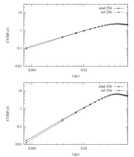
Figure 14: Plots of the first order (top panel) and second order (bottom panel) structure functions of the centroid velocity increment for the neutral species in mf-256 and the bulk flow in mhd-256. Both these clearly follow power laws in $l$ up to lengths of around one quarter of the computational domain.

Simulation	mf-256	mhd-256
$\zeta_{1}$	0.32 (0.71)	0.32 (0.69)
$\zeta_{2}$	0.65 (1.43)	0.65 (1.39)
$\zeta_{3}$	1.00 (2.19)	1.00 (2.14)

Table 5: The exponents of the CVISF${}_{p}(l)$, normalised to $p=3$ for $p=1,2,3$. The numbers in brackets are the absolute exponents.

7 Conclusions

We have presented the results of 4-fluid, MHD turbulence in molecular clouds. The parameters chosen were matched to the observations of molecular clouds reported in Crutcher (1999). We performed a resolution study to ensure that the results presented, in terms of both the power spectra and the RMS Mach number, were not strongly influenced by resolution effects.

We found that the RMS mass-weighted Mach number was not significantly decreased with the inclusion of multifluid effects, in spite of multifluid effects providing an effective pathway for removal of magnetic energy. The overall energy dissipation, then, appears not to be significantly affected by multifluid effects. This phenomenon is a result of the fact that the majority of the energy in a driven, turbulent system with the properties of a molecular cloud resides in kinetic energy and so an enhanced removal of magnetic energy does not significantly effect the global energetics of the system.

We found that both the velocity power spectra of the neutrals and the magnetic field power spectra were strongly influenced by multifluid effects at all length-scales up to the driving scale (0.05 pc). In multifluid MHD, the velocity power spectrum of the neutrals is found to have considerably less structure at all length-scales than those of the charged species. The electron and ion fluids behave almost identically to each other, while the dust displays some slight differences with the other charged species. This latter point arises largely from the requirement of local charge neutrality and the fact that the electrons and ions are the dominant charge carriers in the system. We also find, at very short length-scales, some signs of the Hall effect in the power spectra of the charged species.

Thus we find, in common with the results presented in Papers I and II that multifluid effects are important up to quite large length-scales. This result appears to be in conflict with the observations of Li & Houde (2008) and we deal with this apparent contradiction in a forthcoming paper.

The differences in the power spectra of the bulk densities in the multifluid and ideal MHD systems are not as dramatic as those in the other variables, although there is somewhat less power in the distribution of the neutral density in the multifluid simulation than the bulk density in the ideal MHD one. Interestingly, there is less power in the spectrum of the charged species density than the neutral species in the multifluid system. This is the opposite of what is found for the velocity power spectra.

For all species, and for all cases, the density PDFs are found to be very close to log-normal. The neutral species in the multifluid simulation has a slightly less platykurtic (flattened) distribution than that in the ideal MHD case. The charged densities in the multifluid simulation have, in turn, less platykurtic distributions than the neutrals in that simulation with the dust actually having a leptokurtic distribution. Each of these results is explained in terms of the ambipolar diffusion experienced by the multifluid system, and the fact that the charged species are more directly influenced by the magnetic field than the neutrals.

Finally, we find that multifluid effects do not significantly influence the centroid velocity increment structure functions.

References

- Brunt (2010) Brunt C. M., 2010, A&A, 513, A67
- Brunt, Federrath, & Price (2010a) Brunt C. M., Federrath C., Price D. J., 2010a, MNRAS, 403, 1507
- Brunt, Federrath & Price (2010b) Brunt C. M., Federrath C., Price D. J., 2010b, MNRAS, 405, L56
- Ciolek & Roberge (2002) Ciolek G.E., Roberge W.G., 2002, ApJ, 567, 947
- Crutcher (1999) Crutcher R. M., 1999, ApJ, 520, 706
- Dedner et al. (2002) Dedner A., Kemm F., Kröner D., Munz C.-D., Schnitzer T., Wesenberg M., 2002, JCoPh, 175, 645
- Dib & Burkert (2005) Dib, S. Burkert, A. 2005, ApJ, 446, 665
- Downes & O’Sullivan (2009) Downes, T.P., O’Sullivan, S. 2009, ApJ, 701, 1258, Paper I
- Downes & O’Sullivan (2011) Downes, T.P., O’Sullivan, S. 2011, ApJ, 730, 12, Paper II
- Elmegreen (1993) Elmegreen, B.G. 1993, ApJ, 419, L29
- Elmegreen & Scalo (2004) Elmegreen, B.G., Scalo, J. 2004, ARA&A, 42, 211
- Falle (2003) Falle, S.A.E.G. 2003, MNRAS, 344, 1210
- Federrath, Klessen, & Schmidt (2008) Federrath C., Klessen R. S., Schmidt W., 2008, ApJ, 688, L79
- Federrath et al. (2010) Federrath, C., Duval, J., Klessen, R.S., Schmidt, W., Mac Low, M.-M. 2010, A&A, 512, 81
- Federrath et al. (2011) Federrath C., Chabrier G., Schober J., Banerjee R., Klessen R. S., Schleicher D. R. G., 2011, PhRvL, 107, 114504
- Glover & Mac Low (2007) Glover, S.C.O., Mac Low, M-M. 2007, ApJ, 659, 131
- Gustaffson et al. (2006) Gustaffson, M., Brandenburg, A., Lemaire, J.L., Field, D., 2006, A&A, 454, 515
- Heyer & Brunt (2012) Heyer M. H., Brunt C. M., 2012, MNRAS, 420, 1562
- Hily-Blant, Falgarone, & Pety (2008) Hily-Blant P., Falgarone E., Pety J., 2008, A&A, 481, 367
- Jones & Downes (2012) Jones A. C., Downes T. P., 2012, MNRAS, 420, 817
- Klein et al. (2003) Klein, R.I., Fisher, R.T., Krumholtz, M.R., McKee, C.F. 2003, Winds, Bubbles and Explosions: A conference to honour John Dyson, S.J. Arthur, W.J. Henney, Rev. Mex. Astron. Astrophys., 15, 92
- Klessen (2000) Klessen, R.S. 2000, ApJ, 535, 869
- Kudoh & Basu (2008) Kudoh, T., Basu, S. 2008, ApJ, 679, L97
- Larson (1981) Larson, R.B. 1981, MNRAS, 194, 809
- Lemaster & Stone (2008) Lemaster, M.N., Stone, J.M. 2008, ApJ, 682, L97
- Lemaster & Stone (2009) Lemaster, M.N., Stone, J.M. 2009, ApJ, 691, 1092
- Li & Houde (2008) Li, H.-B, Houde, M. 2008, ApJ, 677, 1151
- Li et al. (2010) Li, H.-B., Houde, M., Lai, S.-P., Sridharan, T.K. 2010, ApJ, 718, 905
- Li et al. (2008) Li, P.S., McKee, C.F., Klein, R.I., Fisher, R.T. 2008, ApJ, 684, 380
- Mac Low (1999) Mac Low, M.-M. 1999, ApJ, 524, 169
- Mac Low & Klessen (2004) Mac Low, M.-M., Klessen, R.S. 2004, Rev. Mod. Phys., 76, 125
- Mac Low et al. (1998) Mac Low, M.-M., Klessen, R.S., Burkert, A., Smith, M.D. 1998 Phys. Rev. Lett., 80, 2754
- Matthaeus et al. (2003) Matthaeus, W.H., Dmitruk, P., Smith, D., Ghosh, S., Oughton, S., 2003, Geophys. Res. Lett. 30(21), 2104
- Mininni et al. (2006) Mininni, P.D., Alexakis, A., Pouquet, A. 2006, Journal of Plasma Physics, 73, 377
- Oishi & Mac Low (2006) Oishi, J.S., Mac Low, M.-M. 2006, ApJ, 638, 281
- Ossenkopf & Mac Low (2002) Ossenkopf V., Mac Low M.-M., 2002, A&A, 390, 307
- Ostriker et al. (2001) Ostriker, E.C., Stone, J.M., Gammie, C.F. 2001, ApJ, 546, 980
- O’Sullivan & Downes (2006) O’Sullivan, S., Downes, T.P. 2006, MNRAS, 366, 1329
- O’Sullivan & Downes (2007) O’Sullivan, S., Downes, T.P. 2007, MNRAS, 376, 1648
- Passot & Vázquez-Semadeni (1998) Passot, T., Vázquez-Semadeni, E. 1998, Phys. Rev. E, 58, 4501
- Price, Federrath, & Brunt (2011) Price D. J., Federrath C., Brunt C. M., 2011, ApJ, 727, L21
- Servidio et al. (2007) Servidio, S., Carbone, V., Primavera, L., Veltri, P., Stasiewicz, K. 2007, P&SS, 55, 2239
- Vázquez-Semadeni (1994) Vázquez-Semadeni, E. 1994, ApJ, 423, 681
- Vestuto et al. (2003) Vestuto, J.G., Ostriker, E.C., Stone, J.M. 2003, ApJ, 590, 858
- Wardle & Ng (1999) Wardle, M., Ng, C. 1999, MNRAS, 303, 239