Particle number fractionalization of a one-dimensional atomic Fermi gas with synthetic spin-orbit coupling

Abstract

We propose an experimental scheme to simulate the fractionalization of particle number by using a one-dimensional spin-orbit coupled ultracold fermionic gas. The wanted spin-orbit coupling, a kink-like potential, and a conjugation-symmetry-breaking mass term are properly constructed by laser-atom interactions, leading to an effective low-energy relativistic Dirac Hamiltonian with a topologically nontrivial background field. The designed system supports a localized soliton excitation with a fractional particle number that is generally irrational and experimentally tunable, providing a direct realization of the celebrated generalized-Su-Schrieffer-Heeger model. In addition, we elaborate on how to detect the induced soliton mode with the fractional particle number in the system.

I introduction

The idea of fractional particle number (FPN) goes back to the Jackiw-Rebbi model Jackiw-Rebbi ; Niemi in the relativistic quantum field theory, where fractionalization of fermion number exhibits when a fermionic field is coupled to a topologically nontrivial background field. The first physical demonstration of this remarkable phenomenon was proposed by Su, Schrieffer, and Heeger (SSH), in which a domain wall in one-dimensional (1D) dimerized polymers, such as polyacetylene, induces a zero-energy soliton state SSH . The particle-hole ambiguity of the zero mode restricts the fractional fermion number to be only $\pm\frac{1}{2}$ in this system hajime ; campbell . Afterwards, achievements have been made to generalize it to an irrational fermion number by introducing another field to break the conjugation symmetry, such as different on-site energies Goldstone ; Jackiw1983 ; rice .

Another famous example of FPN is illustrated in the fractional quantum Hall effect regime Laughin , where the Laughin quasiparticles not only have fractional charges but also have fractional (anyonic) statistics in two dimensions (2D). Recent search for fractionlization in 2D systems has theoretically demonstrated that fractionally charged excitations may exist in graphenelike Chamon , square-lattice Seradjeh and kagome-lattice Ruegg systems with vortex-type order parameters (which describe the mass of the analog Dirac fermions in the systems). The newly discovered quantum spin Hall insulators were also proposed for realizing the SSH model based on the proximity effect, which introduces a magnetic domain-wall Qi2008 ; Vayrynen . Notably, the edge electrons there with the inherent chiral symmetry may exhibit a direct signature of FPN Qi2008 .

On the other hand, quantum simulation of relativistic Dirac Hamiltonian by using ultracold atomic gases has recently attracted great interest Zhang . For example, ultracold fermionic atoms trapped in a honeycomb optical lattice (OL) were theoretically proposed to behave as massless and massive Dirac fermions Zhu2007 , and confirmed in a recent experiment Tarruell . The atomic gases with the synthetic spin-orbit (SO) coupling Lin ; Chen2012 ; Wang2012 ; Cheuk2012 through light-induced gauge fields Dalibard ; Wilczek were also proposed for investigating interesting Dirac dynamics Vaishnav ; Merkl ; cwzhang ; zhang2 ; Zhu2009 ; Goldman . These cold atom systems provide a highly controllable platform for studying a wide range of models in relativistic quantum mechanics and field theory Zhang . Interestingly, Ruostekoski et al. presented an experimental scheme to realize Ruostekoski2002 and detect Ruostekoski2003 the fractionalization of particle number by using a two-component ultracold Fermi gas in a 1D optical superlattice. The low-energy effective theory for the atoms in the system becomes relativistic under certain conditions, and a laser-induced modulation of atomic hopping between neighbor lattices with a kink profile gives rise to a physical domain-wall, leading to soliton modes with FPN.

Inspired by recent experimental achievements in the artificial SO coupling in ultracold bulk bosonic Lin ; Chen2012 and particularly fermionic atoms Wang2012 ; Cheuk2012 , we here present an alternative proposal for realizing the particle number fractionalization using a 1D atomic Fermi gas with the synthetic SO coupling. The required SO interactions and a kink-like potential are properly constructed by dressing atoms with laser beams in the system, such that the low-energy fermionic atoms can behave as massless Dirac fermions coupling to a topologically nontrivial background field. As a result, a localized soliton excitation in the middle of the effective energy gap appears on the domain wall, which is a direct quantum simulation of the standard SSH model. Another two laser beams are used to introduce an effective Zeeman term, which shifts the soliton excitation from the zero-energy. For a midgap state below the zero energy level, it takes more fractional fermion number from the valance band and less from the conduction band, and vice versa for the opposite case, such that the soliton state exhibits an irrational FPN in this general case; moreover, its profile and FPN in the system are experimentally tunable. Furthermore, we suggest experimentally available methods to detect the induced soliton modes with FPN through measuring the soliton density distribution and the local density of states (LDOS) near the kink. We also discuss the possibility of generalizing our proposal to the realization of the FPN in higher spatial dimensions.

The paper is organized as follows. In the next section (Sec. II), we propose an experimental scheme to simulate the generalized SSH model with an irrational FPN by using a 1D SO-coupled atomic Fermi gas. The realization of a relativistic Dirac Hamiltonian with a kink background field is shown, and the induced FPN in the system is calculated and explained. In Sec. III, we elaborate on how to detect the soliton modes with FPN in experiments. Finally, in Sec. IV, we briefly discuss the generalization of the system to higher dimensions and present conclusions.

II simulation of FPN with SO coupled fermionic atoms

In this section, we show how to simulate the fractionalization of particle number by using atomic Fermi gases with the synthetic spin-orbit coupling. Let us start with a brief review of the celebrated model describing kink-soliton states and arbitrary fractional fermion number in the context of relativistic quantum field theory Jackiw-Rebbi ; Goldstone . For 1D massless Dirac fermions subject to two static bosonic fields $\varphi_{1}$ and $\varphi_{2}$, the relativistic Dirac Hamiltonian is given by note1

$$H_{D}=c\sigma_{x}p_{x}-\varphi_{2}(x)\sigma_{y}+\varphi_{1}(x)\sigma_{z},$$ (1)

where $c$ is the effective speed of light and $\sigma_{x,y,z}$ are the Pauli matrices. The background field with a kink potential is described by Goldstone ; Jackiw1983

$$\varphi_{1}(x)=\varphi_{1}^{0},~{}~{}\varphi_{2}(x\rightarrow\pm\infty)=\pm\varphi_{2}^{0},$$ (2)

where $\varphi_{1}^{0}$ and $\varphi_{2}^{0}$ are constants. The kink $\varphi_{2}$ acts as the boundary of two degenerate vacuums Jackiw1983 . The relativistic Dirac Hamiltonian with such a topologically nontrivial background potential supports an unpaired soliton state, which gives rise to fractionalization of particle number Goldstone . Moreover, the FPN is generally irrational and takes one-half in the standard SSH model with the conjugation-symmetry when $\varphi^{0}_{1}$ is vanishing.

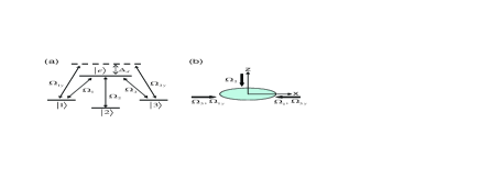
Figure 1: (Color online) Schematic representation of the laser-atom interaction configuration for generating an effective relativistic Dirac Hamiltonian. (a) The three ground states $|1\rangle$, $|2\rangle$ and $|3\rangle$ are resonantly coupled to the excite states $|e\rangle$ by lasers with Rabi frequencies $\Omega_{j}$, and two additional lasers $\Omega_{1y}$ and $\Omega_{3y}$ couples $|1\rangle$ and $|3\rangle$ to $|e\rangle$ with a large detuning $\Delta_{d}$. The choose for the three ground states is that, $|1\rangle$ and $|3\rangle$ are two degenerate Zeeman sublevels which are addressed by laser beams with different polarization and $|2\rangle$ is another hyperfine level with different energy so that it is addressed by a laser with a different frequency. (b) The spatial configuration and propagating direction of the laser beams. The candidate for the fermionic atoms can be ⁶Li or ⁴⁰K.

II.1 Realizing the relativistic Dirac Hamiltonian in cold atom systems

Now we demonstrate how to realize the wanted Dirac Hamiltonian (1) with a SO-coupled atomic Fermi gas. We consider an ensemble of quasi-2D noninteracting fermionic atoms with three relevant spin components in the ground-state manifold $\{|1\rangle,|2\rangle,|3\rangle\}$, which are resonantly coupled to a common excited state $|e\rangle$ through the standard tripod configuration Ruseckas ; zhu2011 as shown in Fig. 1. A candidate for the fermionic atoms can be ⁶Li or ⁴⁰K. For ⁶Li atoms, the hyperfine levels can be selected as

$$\begin{array}[]{ll}|1\rangle=|2^{2}{\text{S}}_{1/2},F=\frac{3}{2},m_{F}=-\frac{1}{2}\rangle,\\ \\ |2\rangle=|2^{2}{\text{S}}_{1/2},F=\frac{1}{2},m_{F}=\frac{1}{2}\rangle,\\ \\ |3\rangle=|2^{2}{\text{S}}_{1/2},F=\frac{3}{2},m_{F}=\frac{3}{2}\rangle,\\ \\ |e\rangle=|2^{2}{\text{P}}_{1/2},F=\frac{1}{2},m_{F}=\frac{1}{2}\rangle.\end{array}$$ (3)

For ⁴⁰K atoms, the corresponding hyperfine levels can be

$$\begin{array}[]{ll}|1\rangle=|4^{2}{\text{S}}_{1/2},F=\frac{7}{2},m_{F}=-\frac{1}{2}\rangle,\\ \\ |2\rangle=|4^{2}{\text{S}}_{1/2},F=\frac{9}{2},m_{F}=\frac{1}{2}\rangle,\\ \\ |3\rangle=|4^{2}{\text{S}}_{1/2},F=\frac{7}{2},m_{F}=\frac{3}{2}\rangle,\\ \\ |e\rangle=|4^{2}{\text{P}}_{1/2},F=\frac{9}{2},m_{F}=\frac{1}{2}\rangle.\\ \\ \end{array}$$ (4)

The corresponding Rabi frequencies of the three resonantly coupling laser beams can be parameterized as

$$\Omega_{1} = \Omega\,\sin\alpha\,\cos\theta\,\mathrm{e}^{-i\kappa x},$$

$$\Omega_{2} = \Omega\,\cos\alpha\,\mathrm{e}^{-i\eta\kappa z},$$ (5)

$$\Omega_{3} = \Omega\,\sin\alpha\,\sin\theta\,\mathrm{e}^{i\kappa x}.$$

The wave numbers are $\kappa$ and $\eta\kappa$ as shown in Fig. 1(a), and $\Omega=\sqrt{\sum_{j=1}^{3}|\Omega_{j}|^{2}}$ is the total Rabi frequency. Here $\eta=1+\delta\eta$ with deviation $\delta\eta$ being for matching the resonant-coupling frequency of the second laser beam. For the selected atomic hyperfine states in Eqs. (3) and (4), $\delta\eta\approx 5\times 10^{-7}$ for ⁶Li atoms and $\delta\eta\approx 3.5\times 10^{-6}$ for ⁴⁰K atoms. This can be achieved in experiments by adjusting the laser frequency. The deviation is negligible in our derivations, however, we still use the notation $\eta$ in the following discussions for consistency. We further adopt uniform plane-wave laser beams that $\Omega$, $\alpha$, and $\theta$ are all constants, and particularly choose $\theta=\pi/4$.

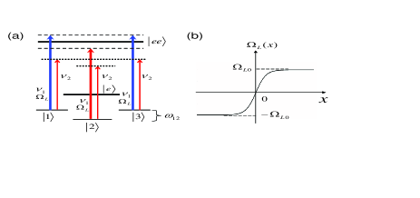
Figure 2: (Color online) Schematic representation of (a) the coupling lasers which generate the wanted external potentials $V_{1,2,3}$ in Eq. (8); and (b) the spatial configuration of the Rabi frequency $\Omega_{L}(x)$ which forms the needed kink-like potential. The frequency difference $\omega_{12}=228$ MHz for ⁶Li atoms and $\omega_{12}=1186$ MHz for ⁴⁰K atoms for the selected hyperfine levels in the text, both of which are much larger than the natural linewidth of the excited state $|ee\rangle$ (about 6 MHz).

The single-particle Hamiltonian for each atom takes the form $H_{s}=\mathbf{p}^{2}/2m_{a}+H_{\text{int}}$, where $\mathbf{p}$ denotes the momentum operator and $m_{a}$ is the atomic mass. The light-atom interaction Hamiltonian $H_{\text{int}}$ is given by $H_{\text{int}}=\hbar\sum_{j=1}^{3}(\Omega_{j}|e\rangle\langle j|+{\text{H.c.}})$. Diagonalizing $H_{\text{int}}$ yields two orthogonal dark states

$$\begin{array}[]{ll}|D_{1}\rangle=\left(\mathrm{e}^{i\kappa x}|1\rangle-\mathrm{e}^{-i\kappa x}|3\rangle\right)\mathrm{e}^{-i\eta\kappa z}/\sqrt{2},\\ |D_{2}\rangle=\left(\mathrm{e}^{i\kappa x}|1\rangle+\mathrm{e}^{-i\kappa x}|3\rangle\right)\mathrm{e}^{-i\eta\kappa z}\cos\alpha/\sqrt{2}-\sin\alpha|2\rangle.\end{array}$$ (6)

The dark states are decoupled to the excited state $|e\rangle$ and thus are immune to spontaneous emission. They span a degenerate subspace, in which the full state of a single atom can be written as $|\chi(\textbf{r})\rangle=\sum_{i=1}^{2}\psi_{i}(\textbf{r})|D_{i}(\textbf{r})\rangle$. The center-of-mass amplitudes $\psi_{i}(\textbf{r})$ corresponding to the spatial wave functions of the two dark states obey the Schrödinger equation $i\hbar\partial_{t}\Phi=H\Phi$, where the two-component spinor $\Phi({\bf r})=(\psi_{1}({\bf r}),\psi_{2}({\bf r}))^{T}$ and the Hamiltonian reads

$$H=\frac{1}{2m_{a}}(\textbf{p}-\textbf{A})^{2}+\phi+V.$$ (7)

The gauge potential $\bf{A}$ arises from the position dependence of the dark states and is given by $\textbf{A}_{j,n}=i\hbar\langle D_{j}(\textbf{r})|\nabla|D_{n}(\textbf{r})\rangle$ Dalibard ; Wilczek . The projecting-induced scalar potential $\phi$ and the external potential $V$ are respectively determined by $\phi_{j,n}=\sum_{l=1}^{2}\vec{A}_{j,l}\vec{A}_{l,n}/2m_{a}$ and $V_{j,n}=\langle D_{j}(\textbf{r})|\hat{V}|D_{n}(\textbf{r})\rangle$ with $\hat{V}=\sum_{l=1}^{3}V_{l}(\textbf{r})|i\rangle\langle i|$ Dalibard ; Wilczek . We consider the adiabatic motion of atoms initially prepared in the dark state subspace. It should be noted that the two dark states are not the lowest energy states in this system so that the adiabatic approximation works well only for finite time scales (mainly due to collisional relaxations), up to several hundred milliseconds under realistic conditions zhu2011 . To obtain a lowest-energy two-fold (nearly) degenerate subspace, one can adopt the optical dressing scheme described in Ref. zhang2 (where atoms with simpler $\Lambda$ type configuration) or in Ref. Juzeliunas (where more atomic internal states and coupling lasers are required).

The Rabi frequencies chosen in Eq.(5) can realize the first term in Hamiltonian (1) with certain potentials; however, to implement the required potentials exactly in Eq.(1), more complicated laser configures are needed. One possible method to generate the required potentials is that we further choose two additional laser beams with frequencies $\nu_{1}$ and $\nu_{2}$, as schematically shown in Fig. 2(a). The first laser beam (denoted by frequency $\nu_{1}$) with the effective Rabi frequency $\Omega_{L}$ (which takes the real Rabi frequency and the detuning into account) is blue detuned for atoms in the internal levels $|1\rangle$ and $|3\rangle$, but red detuned for atoms in level $|2\rangle$, all of which are far-off-resonantly coupled to another excited state $|ee\rangle$. This energy state can be selected as $|ee\rangle=|2^{2}{\text{P}}_{3/2},F=\frac{3}{2},m_{F}=\frac{1}{2}\rangle$ for ⁶Li atoms and $|ee\rangle=|4^{2}{\text{P}}_{3/2},F=\frac{9}{2},m_{F}=\frac{1}{2}\rangle$ for ⁴⁰K atoms, respectively. In addition, the second laser (denoted by frequency $\nu_{2}$), which is also far-off-resonant, is use to create constant energy terms in $V_{1,3}$ and $V_{2}$ in the following equation (8). The energy difference between them [cf. Eq. (8)] can be realized by detuning the second laser from the two-photon resonance with the frequency $\hbar\kappa^{2}(1-\eta^{2}\cos^{2}\alpha)/2m_{a}$. Thus the resulting external potentials are given by

$$\begin{array}[]{ll}V_{1}=V_{3}=\hbar\Omega_{L}(x,z)-\frac{\hbar^{2}\kappa^{2}}{2m_{a}},\\ \\ V_{2}=-\hbar\Omega_{L}(x,z)-\frac{\hbar^{2}\eta^{2}\kappa^{2}}{2m_{a}}\cos^{2}\alpha.\end{array}$$ (8)

After introducing all of the laser configurations, we can obtain the total resulting potentials for the atoms in the laser field as

$$\begin{array}[]{ll}\textbf{A}=-\hbar\kappa\cos\alpha\ \sigma_{x}\vec{e}_{x}+\hbar\eta\kappa\left(\begin{array}[]{cc}1&0\\ 0&\cos^{2}\alpha\end{array}\right)\vec{e}_{z},\\ \\ \phi=\frac{\hbar^{2}\kappa^{2}\sin^{2}\alpha}{2m_{a}}\left(\begin{array}[]{cc}1&0\\ 0&\eta^{2}\cos^{2}\alpha\end{array}\right),\\ \\ V=\left(\begin{array}[]{cc}V_{1}&0\\ 0&V_{1}\cos^{2}\alpha+V_{2}\sin^{2}\alpha\end{array}\right),\end{array}$$ (9)

with $\phi+V=\hbar\Omega_{L}\sin^{2}\alpha\sigma_{z}$ up to an irrelevant constant. Note that atoms in such a synthetic non-Abelian gauge field behave as electrons with a SO coupling, which can be seen from the term $\textbf{p}\cdot\textbf{A}$ in Hamiltonian (7).

By applying an additional extremely anisotropic trapping potential to freeze the atomic motions along $z$ axis, we arrive at the quasi-1D cases note2 . For ultralow temperature, the momentum of atoms along $x$ axis $p_{x}\ll\hbar\kappa\cos\alpha$, such that the $p_{x}^{2}$ term in Eq. (7) may be safely neglected, leading to an effective Dirac Hamiltonian

$$H_{e}\approx c_{x}\sigma_{x}p_{x}+\Delta(x)\sigma_{z},$$ (10)

where $c_{x}=\hbar\kappa\cos\alpha/m_{a}$ is the effective speed of light in this system and $\Delta(x)=\hbar\Omega_{L}(x)\sin^{2}\alpha$. The Hamiltonian (10) describes a massive Dirac fermion having a position-dependent mass $\Delta(x)/c_{x}^{2}$, or in another point of view, a massless Dirac fermion coupling to a static background field $\Delta(x)$ Jackiw-Rebbi . If we choose the intensity distribution of the laser beam with photon frequency $\nu_{1}$ as a kink-type function along $x$ axis, then the standard SSH model in continuum limit SSH is realized in this cold atom system. It is interesting to note that the laser-atom interaction of $\Lambda$ configuration zhang2 can also be used to realize the relativistic Dirac Hamiltonian (10), and in this case the experimental setup can even be simpler. While it is noted that such a simplified scheme is unable to be extended to realize the generalized SSH model described in Eq. (11) below with an irrational FPN.

To introduce the constant field $\varphi^{0}_{1}$ in Hamiltonian (1), which acts as a mass term and breaks the conjugation symmetry, we can apply two additional laser beams to couple the atomic states $|1\rangle$ and $|3\rangle$ to the excited state $|e\rangle$ off-resonantly with a large detuning $\Delta_{d}$ as shown in Fig. 1, with the corresponding Rabi frequencies $\Omega_{1y}=i\left|\Omega_{y}\right|\mathrm{e}^{i\kappa x}$ and $\Omega_{3y}=\left|\Omega_{y}\right|\mathrm{e}^{-i\kappa x}$ zhu2011 . Since $\left|\Omega_{1y}\right|,\left|\Omega_{3y}\right|\ll\Delta_{d}$, the effective Hamiltonian describes a perturbation coupling between states $|1\rangle$ and $|3\rangle$, which is given by $H_{p}=-i\hbar\Omega_{p}e^{2i\kappa x}|1\rangle\langle 3|+{\text{H.c.}}$ with $\Omega_{p}=|\Omega_{y}|^{2}/\Delta_{d}$ note3 . We assume $\Omega_{p}\ll\Omega$, so the Hamiltonian $H_{p}$ can not pump the atoms outside of the dark state subspace. Mapping $H_{p}$ into the subspace spanned by the basis $\{|D_{1}\rangle,|D_{2}\rangle\}$, we obtain $H_{p}=\hbar\Omega_{p}\cos\alpha\sigma_{y}$. Therefore, the total 1D effective Hamiltonian for the ultracold atoms is ${H}_{\text{1D}}=H_{e}+H_{p}$. By introducing a unitary transformation $\Phi(x)\rightarrow e^{i\frac{\pi}{4}\sigma_{x}}\Phi(x)$, we can obtain the Dirac Hamiltonian

$${H}_{\text{1D}}=c_{x}\sigma_{x}p_{x}+\Delta(x)\sigma_{y}-\Gamma\sigma_{z},$$ (11)

where $\Gamma=\hbar|\Omega_{y}|^{2}\cos\alpha/\Delta_{d}$. We note that the unitary transformation used here is for mathematical convenience but involves no manipulation on the system. Compared to the original Dirac Hamiltonian (1), here the effective field $-\Gamma$ corresponds to the constant background $\varphi^{0}_{1}$, and the field $\Delta(x)$ should present a kink-like profile, which corresponds to $-\varphi_{2}(x)$. To this end, we can choose the spatial profile of the Rabi frequency $\Omega_{L}(x)$ with the kink form as shown in Fig. 2(b), and $\Omega_{L}(x)=\pm\Omega_{L0}$ as $x\rightarrow\pm\infty$. Thus the asymptotic value of $\Delta(x)$ can be denoted as $\Delta_{0}\equiv\Delta(x\rightarrow+\infty)=\hbar\Omega_{L0}\sin^{2}\alpha$.

Finally in this section, we note that the recent experiment of generating SO couplings in Fermi gases Wang2012 may also be extended to realize the Dirac Hamiltonians (10) and (11). In the experiment Wang2012 , two spin-1/2 states are chosen as two internal hyperfine states instead of dressed states [see Eq. (6)] in our scheme, and they are coupled by a pair of Raman beams with spatially homogenous coupling strength $\Omega_{R}$. The synthetic SO coupling is just one-dimensional with the form $p_{x}\sigma_{z}$, and there is an additional term related to the Raman coupling $\Omega_{R}\sigma_{x}$ in the single-particle Hamiltonian (see Refs. Lin ; Wang2012 for details). If one uses Raman beams with spatially imhomogenous coupling strength and kink-type profile along $x$ axis [i.e. $\Omega_{R}(x)=\Omega_{L}(x)$], the low-energy effective Hamiltonian for the atoms takes the form of the Dirac Hamiltonian (10) under a spin rotation. To simulate the generated SSH model Hamiltonian (11), one needs additional laser beams or radio-frequency fields to couple the two spin states as a $\sigma_{y}$-coupling term.

II.2 Fractional particle number in this system

We now turn to calculate the FPN in the proposed system. There is a number of methods for computing the FPN of topological solitons Niemi , including the well-known conjugation-symmetry analysis for the zero modes with one-half fermion number Niemi ; Jackiw2 . It was first pointed out by Goldstone and Wilczek that Goldstone , at zero temperature, the fractional fermion number of the soliton in this model is determined by the kink background field (2). The adiabatic condition was imposed there for a valid perturbation calculation by assuming $|\partial\varphi_{i}|\ll m^{2}$ ($i=1,2$), where $m\equiv\sqrt{\varphi_{1}^{2}+\varphi_{2}^{2}}$. However, Yamagishi showed that the exact result actually does not depend on the adiabatic condition Yamagishi . For simplicity, we here employ still the adiabatic condition to derive the result in a new but simple way. The current of this (1+1)D system is

$$j^{\mu}(x)=-\langle x|\mathbf{tr}\gamma^{\mu}\widehat{G}|x^{+}\rangle,$$ (12)

where the Dirac matrices $\gamma^{0}=\sigma_{z}$, $\gamma^{1}=i\sigma_{y}$, $\gamma^{5}=\sigma_{x}$, and the Green’s function of the relativistic Dirac Hamiltonian (1) is given by

$$G=\frac{i}{\gamma^{\mu}\hat{p}_{\mu}-(\varphi_{1}+i\varphi_{2}\gamma^{5})}.$$ (13)

Here $\mu=0,1$ correspond to the time and space components, respectively.

In the derivation, we have used the adiabatic approximation that $\partial\varphi_{i}$ commutes with $\frac{1}{\hat{p}^{2}-m^{2}}$ and kept the first order approximation. Thus the Green’s function can be written as

$$\begin{array}[]{ll}G=[\gamma^{\mu}\hat{p}_{\mu}+(\varphi_{1}-i\varphi_{2}\gamma^{5})]\{G^{-1}[\gamma^{\mu}\hat{p}_{\mu}+(\varphi_{1}-i\varphi_{2}\gamma^{5})]\}^{-1}\\ \\ ~{}~{}\approx\left[\gamma^{\mu}\hat{p}_{\mu}+(\varphi_{1}-i\varphi_{2}\gamma^{5})\right]\frac{i}{\hat{p}^{2}-m^{2}}\\ \\ ~{}~{}~{}~{}~{}-\left[\gamma^{\mu}\hat{p}_{\mu}+(\varphi_{1}-i\varphi_{2}\gamma^{5})\right]\frac{1}{(\hat{p}^{2}-m^{2})^{2}}\gamma^{\nu}\partial_{\nu}(\varphi_{1}-i\varphi_{2}\gamma^{5}).\end{array}$$ (14)

After a straightforward calculation, given that the chemical potential (the Fermi level) is zero, we can obtain the average current in the background field as Goldstone

$$j^{\mu}(x)=-\frac{1}{2\pi}\epsilon^{\mu\nu}\partial_{\nu}\Theta(x),$$ (15)

where $\Theta(x)=\arg(\varphi_{1}+i\varphi_{2})$ denotes the angular field of the background, and $\epsilon^{\mu\nu}$ is the two-index totally antisymmetric tensor. When the chemical potential $\tilde{\mu}=0$, the particle density is given by $\rho_{0}(x)=-\frac{1}{2\pi}\frac{\partial\Theta(x)}{\partial x}$ with respect to the density of kink-free system. Thus we obtain the FPN $\mathcal{N}_{0}=\int\rho_{0}(x)dx$ in this system with $\varphi_{1}^{0}=-\Gamma$ and $\varphi_{2}(x)=-\Delta(x)$ as

$$\mathcal{N}_{0}=\frac{1}{\pi}\arctan\left(\frac{\Delta_{0}}{-\Gamma}\right)=-\frac{1}{\pi}\arctan\left(\frac{\Omega_{L0}\Delta_{d}\sin^{2}\alpha}{|\Omega_{y}|^{2}\cos\alpha}\right).$$ (16)

It is clear from Eq. (16) that $\mathcal{N}_{0}$ is generally irrational and can be an arbitrary fractional number in the range $(-\frac{1}{2},\frac{1}{2})$ for a finite $\Gamma$. Especially, the conjugation-symmetric Jackiw-Rebbi model is obtained in the limit $\Gamma\rightarrow 0$, i.e., without applying the laser beams $\Omega_{{\text{1}y}}$ and $\Omega_{{\text{3}y}}$. In this case, the soliton is a zero-energy mode with one-half fermion number $\mathcal{N}_{0}=\pm\frac{1}{2}$. It is interesting to note that the FPN in this system is widely tunable in experiments via laser-atom interactions [cf. Eq. (16)], making it a controllable platform for simulating fractionalization of particle number.

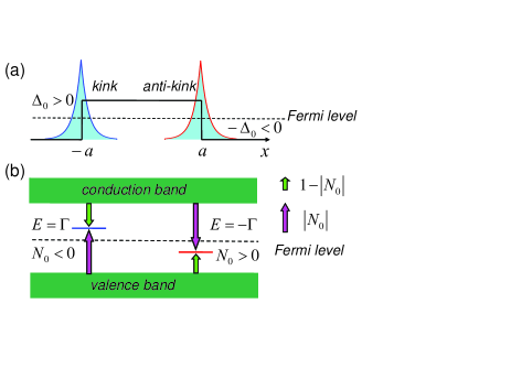
Figure 3: (Color online) Schematic representation of (a) a background field with a pair of kink and anti-kink, both of which support a localized soliton state with profile $\sim\exp{(-\Delta_{0}|x\pm a|/\hbar c_{x})}$; and (b) the energy spectrum and a pair of solitons with energies $E=\pm\Gamma$ and fractional particle numbers $\pm|\mathcal{N}_{0}|$. The midgap soliton modes are protected by an energy gap $E_{g}=2\sqrt{\Delta^{2}_{0}+\Gamma^{2}}$ between the effective conduction band and valence band. At the kink, the soliton state picks a FPN of $|\mathcal{N}_{0}|$ from the effective valance band and another $1-|\mathcal{N}_{0}|$ from the effective conduction band, and vice versa for the opposite case at the anti-kink.

Fractionalization has been widely investigated in relativistic quantum field theory Jackiw ; Niemi and condensed matter systems SSH ; Goldstone ; Jackiw1983 ; rice ; Laughin ; Chamon ; Seradjeh ; Ruegg ; Qi2008 ; Vayrynen , where it can give rise to interesting transport phenomena. For example, the existence of fractionally charged excitations greatly enhances the conductivity in the polymers SSH and may induce quantized currents in the quantum spin Hall insulators Qi2008 . The interpretation of FPN in these kink-soliton systems is usually in terms of deformation (or polarization) of the ground-state vacuum due to the kink which supports a single soliton mode Niemi ; Jackiw . This fractionalization mechanism is very different from that in the fractional quantum Hall effect regime, where the fractional collective excitations are described by a strongly correlated Laughlin wave function Laughin .

To have better understanding of this mechanism, we consider another kind of background field with a simple but experimentally practical configuration, that is, a pair of kink and anti-kink both with a step-function profile as shown in Fig. 3(a). Here we assume $\Delta_{0}>0$ and $a\gg\hbar c_{x}/\Delta_{0}$ such that the kink and anti-kink are almost decoupled. By solving the energy spectrum of Hamiltonian (11) at the kink potential (near $x=-a$) with $\Delta(x)=\Delta_{0}\textbf{sgn}(x+a)$, we find that there is a localized midgap eigenstate in the kink at $E=\Gamma$ with the wavefunction decaying as $\exp{(-\Delta_{0}|x+a|/\hbar c_{x})}$ and the energy gap $E_{g}=2\sqrt{\Delta^{2}_{0}+\Gamma^{2}}$ . It is understood that the isolated state picks up a fractional fermion number (i.e., FPN) of $|\mathcal{N}_{0}|$ [see Eq. (16)] from the effective valance band and $(1-|\mathcal{N}_{0}|)$ from the effective conduction band, as shown in Fig. 3(b). For an anti-kink potential (near $x=a$) with $\Delta(x)=-\Delta_{0}\textbf{sgn}(x-a)$, the localized soliton state is obtained at $E=-\Gamma$ with the wavefunction decaying as $\exp{(-\Delta_{0}|x-a|/\hbar c_{x})}$ as shown in Fig. 3(a). It picks up $(1-|\mathcal{N}_{0})|$ from the valence band and $|\mathcal{N}_{0}|$ from the conduction band. For a periodic system, there must be pairs of kink and anti-kink. If both states are unoccupied, the particle numbers are $-|\mathcal{N}_{0}|$ at the kink and $|\mathcal{N}_{0}|-1$ at the anti-kink. When the chemical potential, i.e., the effective Fermi level in this system, is tuned up, the $E=-\Gamma$ soliton state is occupied first and the particle numbers at kink and anti-kink are $\mp|\mathcal{N}_{0}|$, respectively. And when both states are occupied, there are particles $(1-|\mathcal{N}_{0}|)$ and $|\mathcal{N}_{0}|$ at the kink and anti-kink.

From Eq. (16), we can see that the FPN $\mathcal{N}_{0}$ depends only on the asymptotic value of the kink $\Delta_{0}$ rather than the detailed shape of $\Delta(x)$. In this sense, it is topological and is insensitive to local fluctuations of the background field. This property enables us to use laser beams of different and imperfect intensity distributions compared to the ones with the exact kink profile as shown in Fig. 2(b) and with a wide square-potential profile of a kink-anti-kink pair as shown in Fig. 3(a). In experiments, the intensity distribution of laser beams can be well designed and the wanted ones with nearly square-potential profiles have been realized Tarallo . Although the value of $\mathcal{N}_{0}$ is obtained at zero temperature, the corresponding FPN for finite temperature $T$ defined as $\mathcal{N}_{T}$ can also be calculated by taking the thermal distribution (i.e., Dirac-Fermi distribution) into account Dunne . Interestingly, $\mathcal{N}_{T}$ is just depends on the asymptotic value of the background field and the temperature $T$ Dunne . At low temperatures, i.e., $|\varphi^{0}_{1}|\beta\gg 1$ with $\beta=1/k_{B}T$ ($k_{B}$ is the Boltzmann constant), one has $\mathcal{N}_{T}\approx\mathcal{N}_{0}-e^{-|\varphi^{0}_{1}|\beta}$Dunne . For our proposed cold atom system with the typical temperature $T\sim 0.1$ $\mu$k and parameter $\Gamma/\hbar\sim 0.1$ MHz, the deviation $\mathcal{N}_{0}-\mathcal{N}_{T}\approx e^{-\Gamma\beta}\approx e^{-10}$. Thus we can conclude that the FPN in this system is very robust against the finite-temperature modification due to the gap protection.

Before ending this section, we discuss briefly the modifications on the soliton state and its FPN arising from the neglected quadratic term in the Dirac Hamiltonian (10). For this system of bulk atomic gases, the effective cutoff momentum is determined by the Fermi level and the typical atomic momentum can be one order less than the recoil momentum of photons (for temperature $T\sim 0.1$ $\mu$k and $\kappa\cos\alpha\sim 10^{7}$ ${\text{m}}^{-1}$). So we can treat it as a perturbation $\delta H=p_{x}^{2}/2m_{a}$. This perturbation alters the energy spectrum and also breaks the conjugation symmetry, but the Dirac point and the energy gap opened by the kink-background remain. From the perturbation calculations, we find that both of the spatial profile and the energy of the soliton state are modified. For the case of step-function kink potential and when $\Gamma=0$, the spatial wavefunction of the soliton state decays as $\left[1+\frac{\Delta_{0}}{4m_{a}c^{2}_{x}}(1+\frac{\Delta_{0}|x+a|}{\hbar c_{x}})\right]\exp{(-\Delta_{0}|x+a|/\hbar c_{x})}$, which is slightly broader than that in the absence of $\delta H$ [c.f. Fig. 3(a)]. The corresponding energy is shifted from $E=0$ to $E=-\Delta_{0}^{2}/2m_{a}c_{x}^{2}$ up to the first order perturbation. As long as this energy shift is very small compared to the gap, i.e. $\Delta_{0}/2m_{a}c^{2}_{x}\ll 1$, one can expect that the soliton state is robust against the breaking of conjugation symmetry induced by the quadratic term Chamon . In this case, the modification of FFN can be estimated as $\delta\mathcal{N}_{0}\approx\left|\frac{1}{2}-\frac{1}{\pi}\arctan(\frac{2m_{a}c^{2}_{x}}{\Delta_{0}})\right|$. The situation is more complicated for $\Gamma\neq 0$, but one can still follow a similar perturbation argument and obtain the corresponding modification of the soliton state at the kink.

III detection of soliton with FPN

In this section, we propose possible methods for detecting the fractionalization of particle number in the atomic system mainly through the soliton density and the LDOS near the kink (or the anti-kink) by using two standard experimental detection methods for ultracold atomic gases, such as in-situ absorption imaging technique Bartenstein and spatially resolved radio-frequency (rf) spectroscopy Shin .

First, the density distribution of the soliton modes may be extracted out from the atomic density measurement via optical in-situ absorption imaging Bartenstein . In this continuum model, we work in the soliton framework, and the physical particle number in the soliton sector is equivalently defined as being measured relative to the free sector without the kink background Jackiw1983 ; Jackiw . Thus the density distribution of the soliton mode is given by Jackiw1983 ; Jackiw

$$\begin{array}[]{ll}\rho_{0}(x)=\int dE\left[|\Psi_{E}(x)|^{2}-|\psi_{E}(x)|^{2}\right]\\ \\ ~{}~{}~{}~{}~{}~{}~{}=\left.\left[\tilde{\Upsilon}(x)-\Upsilon(x)\right]\right|_{E_{F}=0},\end{array}$$ (17)

where $\Psi_{E}$ ($\psi_{E}$) and $\tilde{\Upsilon}(x)$ [$\Upsilon(x)$] are the fermion single-particle energy eigenstates and atomic density distribution in the presence (absence) of kink background $\varphi_{2}(x)$, respectively. Note that here we have assumed the effective Fermi level at $E_{F}=0$, which can be achieved by properly tuning the chemical potential of the atomic gas. In this sense, we can measure the spatial density distribution of the SO-coupled Fermi gas both with and without the kink potential by tuning on and off the laser beam $\Omega_{L}$, which correspond to $\tilde{\Upsilon}(x)$ and $\Upsilon(x)$, respectively. The integration of $\rho_{0}(x)$ gives the value of FPN $\mathcal{N}_{0}$ in Eq. (16). This detection scheme provides a clear physical picture of FPN; however, it is hard to be implemented in a practical experiment, as there is only one atom in the soliton sector (kink and anti-kink) comparing to $N_{a}-1$ ones in the free sector, where the total number of fermions $N_{a}$ is restricted by the chemical potential and is usually several orders larger than unit. In addition, the number of soliton modes can not be scaled with increasing $N_{a}$. However, the occupation of the soliton state affects significantly the atomic density distribution near the kink, which may be regarded as a convenient feature to identify the existence of solitons.

An alternative but practical approach to probe the soliton state is measuring the LDOS $\rho(x,E)$ near the kink (or anti-kink) by using spatially resolved rf spectroscopy Shin , which has been proposed to detect other midgap bound states in bulk Fermi gases Jiang , including the zero-energy Majorana modes zhu2011 ; Tewari ; Liu . The idea is that one first uses a probe rf field to induce a single-particle excitation from the initial state $|a_{i}\rangle$ to an unoccupied fluorescent probe state $|a_{f}\rangle$, and then imaging the population in state $|a_{f}\rangle$ to obtain the spatial information about the LDOS Shin ; Jiang ; Liu . If we assume that the probe field is weak and is detuning $\delta_{\text{rf}}$ from the the induced transitions, then the population change in state $|a_{f}\rangle$ can be calculated from the linear response theory Jiang ; Liu

$$I(x,E)\equiv\frac{d}{dt}\langle a^{{\dagger}}_{f}(x)a_{f}(x)\rangle\propto\rho_{a_{i}}(x,E-\delta_{\text{rf}})\Xi(\delta_{\text{rf}}-E),$$ (18)

where $\Xi(\cdot)$ is a unit step function. For a harmonically trapped gas, the chemical potential changes from $\tilde{\mu}=0$ here to $\tilde{\mu}(x)=\frac{1}{2}m_{a}\omega^{2}x^{2}$ with $\omega$ being the trapping frequency under the local density approximation, and $E$ in Eq. (18) is thus replaced by $E-\tilde{\mu}(x)$. Due to the trapping potential, the energy variation over the length scale $l_{0}\equiv\sqrt{E_{g}/m_{a}\omega^{2}}$ becomes comparable to the energy gap which protects soliton modes. Therefore we could use a sufficiently weak trap and experimentally control the size of the gap to reach the nonvanishing gap and locally homogeneous limit. Thus the previously presented physical picture about the soliton mode persists. Since the soliton mode in the proposed system has energy $\Gamma$ inside the gap and is localized at the kink $x=-a$, there will be a significantly enhanced population transfer with frequency $\delta_{\text{rf}}/\hbar=[\Gamma-\tilde{\mu}(-a)]/\hbar$ near the kink. The contribution from the soliton mode would be clearly visible and well separated from other quasiparticle contributions by the energy gap $E_{g}$. Thus the soliton density distribution $\rho_{0}(x,\Gamma)$ can be mapped and singled out in this way. Compared with the previous detection method, the later scheme is insensitive to the fluctuations in the initial number of fermions $N_{a}$ since (i) the occupation of the soliton mode just depends on the Fermi level (i.e. the chemical potential at the kink) and the fluctuations of $N_{a}$ will not affect the topology of the Fermi level; (ii) the soliton mode is an eigenstate that is robust against thermal and local fluctuations in the presence of an energy gap. Interestingly, even single atom in $|a_{f}\rangle$ state can be detected with the standard quantum jump technique if $|a_{f}\rangle$ is selected to be a different hyperfine state zhu2011 ; Tewari . Furthermore, this rf spectroscopy technique works as an analog of the powerful scanning tunneling microscope for probing the atomic gases Shin ; Jiang : another atom will occupy the soliton state after the original atom is scattered out by the probing laser. Therefore, although there is only one atom in the kink and anti-kink at a time, the population in $|a_{f}\rangle$ increases with the probing time. Therefore, this scheme can be easily implemented in a practical experiment. In this method, FPN can be indirectly deduced from the population of the soliton state and then it is actually an indirect method to measure FPN.

IV discussion and conclusion

Before concluding this paper, we discuss briefly how to realize the FPN in 2D and 3D relativistic quantum field theories Jackiw2 . It has been shown that a 2D Dirac Hamiltonian with a vortex-like spatially inhomogenous mass term also supports a zero-energy mode with one-half fermion number Chamon ; Seradjeh ; Ruegg ; Jackiw2 . The wanted 2D SO coupling acting as the kinetic term in the Dirac Hamiltonian can be generated in the previous laser-atom interaction configuration, such as $c_{x}\sigma_{x}p_{x}-c_{z}\sigma_{z}p_{z}$ with $c_{z}=\frac{1}{2}\eta\hbar\kappa\sin^{2}\alpha$. Other kinds of SO coupling terms can also be generated via appropriate optical dressing Dalibard . Another crucial step is to simulate the position-varying mass term with vortex profiles Jackiw2 . Specifically in this cold atom system, one needs $\Omega_{L}(x,z)$ with profiles of the vortex type in contrast to the kink type for 1D cases shown in Eq. (11). Fortunately, the needed laser fields with vortex type defects can be created by using the so-called optical vortex technique OV , which moreover has been implemented in cold atomic gases in experiments Wright .

FPN can also be present in 3D Dirac systems, where the topologically non-trivial background field should be replaced by a 3D profile of a magnetic monopole Jackiw-Rebbi ; Jackiw2 . For the 3D cases, we need the SO coupling term such as $\sigma_{x}p_{x}+\sigma_{y}p_{y}+\sigma_{z}p_{z}$, which can be synthesized by the atom-light-interaction scheme proposed in Ref. 3DSOC . The wanted mass term with monopole profiles may be generated by using electromagnetic field superpositions like those were used to induce 3D Skyrmions in atomic gases Ruostekoski .

In summary, we have proposed an experimental scheme to realize the fractionalization of particle number with a 1D SO-coupled ultracold Fermi gas. A kink-like potential and a conjugation-symmetry breaking mass term are constructed by proper laser-atom interactions, leading to an effective low-energy relativistic Dirac Hamiltonian with a topologically nontrivial background field. As a result, a localized soliton mode emerges near the kink, having an FPN which is generally irrational and experimentally tunable. The proposed cold atomic system provides a direct quantum simulation of the famous generalized SSH model. We have also presented two useful methods to detect the induced soliton modes and the FPN in the system. In view of the fact that SO-coupled Fermi gases were realized in two very recent experiments Wang2012 ; Cheuk2012 , it is anticipated that the present proposal will be tested experimentally in near future.

V acknowledgments

We thank C.-Y. Hou, C. Chamon and Y. Chen for helpful discussions. This work was supported by the NSFC (Grants No. 11125417, No. 10974059, No. 11104085, No. 91121023, and No. 11004065), the SKPBR (Grant No. 2011CB922104), the GRF (HKU7058/11P) and CRF (HKU-8/11G) of the RGC of Hong Kong.

References

- (1) R. Jackiw and C. Rebbi, Phys. Rev. D 13, 3398 (1976).
- (2) For a review, see A. Niemi and G. Semenoff, Phys. Rep. 135, 99 (1986).
- (3) W. P. Su, J. R. Schrieffer, and A. J. Heeger, Phys. Rev. Lett. 42, 1698 (1979); A. J. Heeger, S. Kivelson, J. R. Schrieffer, and W. P. Su, Rev. Mod. Phys. 60, 781 (1988).
- (4) H. Takayama, Y. R. Lin-Liu and K. Maki, Phys. Rev. B 21, 2388 (1980).
- (5) D. K. Campbell and A. R. Bishop, Phys. Rev. B 24, 4859 (1981).
- (6) J. Goldstone and F. Wilczek, Phys. Rev. Lett. 47, 986 (1981)
- (7) R. Jackiw and G. Semenoff, Phys. Rev. Lett. 50, 439 (1983).
- (8) M. J. Rice and E. J. Mele, Phys. Rev. Lett. 49, 1455 (1982).
- (9) R. B. Laughin, H. Störmer, and D. Tsui, Rev. Mod. Phys. 71, 863 (1988).
- (10) C. Chamon, Phys. Rev. B 62, 2806 (2000); C.-Y. Hou, C. Chamon, and C. Mudry, Phys. Rev. Lett. 98, 186809 (2007); C. Chamon, C.-Y. Hou, R. Jackiw, C. Mudry, S.-Y. Pi, and G. Semenoff, Phys. Rev. B 77, 235431 (2008); R. Jackiw and S.-Y. Pi, Phys. Rev. B 78, 132104 (2008).
- (11) B. Seradjeh, C. Weeks, and M. Franz, Phys. Rev. B 77, 033104 (2008).
- (12) A. Rüegg and G. A. Fiete, Phys. Rev. B 83, 165118 (2011).
- (13) X.-L. Qi, T. L. Hughes, and S.-C. Zhang, Nat. Phys. 4, 273 (2008).
- (14) J. I. Väyrynen and T. Ojanen, Phys. Rev. Lett. 107, 166804 (2011).
- (15) For a review, see D. W. Zhang, Z. D. Wang, and S. L. Zhu, Front. Phys. 7, 31 (2012), and the references therein.
- (16) S. L. Zhu, B. Wang, and L.-M. Duan, Phys. Rev. Lett. 98, 260402 (2007); K. L. Lee, B. Gremaud, R. Han, B. G. Englert, and C. Miniatura, Phys. Rev. A 80, 043411 (2009); A. Bermudez, N. Goldman, A. Kubasiak, M. Lewenstein, M. A. Martin-Delgado, New J. Phys. 12, 033041 (2010).
- (17) L. Tarruell, D. Greif, T. Uehlinger, G. Jotzu, T. Esslinger, Nature (Landon), 483, 303 (2012).
- (18) Y.-J. Lin, K. Jiménez-García, and I. B. Spielman, Nature (London) 471, 83 (2011).
- (19) S. Chen, J.-Y. Zhang, S.-C. Ji, Z. Chen, L. Zhang, Z.-D. Du, Y.-J. Deng, H. Zhai, J.-W. Pan, arXiv: 1201.6018.
- (20) P. Wang, Z.-Q. Yu, Z. Fu, J. Miao, L. Huang, S. Chai, H. Zhai, and J. Zhang, Phys. Rev. Lett. 109, 095301 (2012).
- (21) L. W. Cheuk, A. T. Sommer, Z. Hadzibabic, T. Yefsah, W. S. Bakr, M. W. Zwierlein, 109, 095302 (2012).
- (22) J. Dalibard, F. Gerbier, G. Juzeliünas, and P. Öhberg, Rev. Mod. Phys. 83, 1523 (2011).
- (23) F. Wilczek and A. Zee, Phys. Rev. Lett. 52, 2111 (1984); C. P. Sun and M. L. Ge, Phys. Rev. D 41, 1349 (1990).
- (24) J. Y. Vaishnav and C. W. Clark, Phys. Rev. Lett. 100, 153002 (2008); G. Juzeliūnas, J. Ruseckas, M. Lindberg, L. Santos, and P. Öhberg , Phys. Rev. A 77, 011802(R) (2008).
- (25) M. Merkl, A. Jacob, F. E. Zimmer, P. Öhberg, and L. Santos, Phys. Rev. Lett. 104, 073603 (2010).
- (26) Y. Zhang, L. Mao, and C. Zhang, Phys. Rev. Lett. 108, 035302 (2012).
- (27) S. L. Zhu, H. Fu, C. J. Wu, S. C. Zhang, and L. M. Duan, Phys. Rev. Lett. 97, 240401 (2006); D. W. Zhang, Z. Y. Xue, H. Yan, Z. D. Wang, and S. L. Zhu, Phys. Rev. A 85, 013628 (2012).
- (28) S. L. Zhu, D. W. Zhang, and Z. D. Wang, Phys. Rev. Lett. 102, 210403 (2009); M. J. Edmonds, J. Otterbach, R. G. Unanyan, M. Fleischhauer, M. Titov, and P. Öhberg, e-print arXiv: 1106.5925.
- (29) N. Goldman, A. Kubasiak, A. Bermudez, P. Gaspard, M. Lewenstein, and M. A. Martin-Delgado, Phys. Rev. Lett. 103, 035301 (2009); F. Mei, S. L. Zhu, Z.-M. Zhang, C. H. Oh, and N. Goldman, Phys. Rev. A 85, 013638 (2012).
- (30) J. Ruostekoski, G. V. Dunne, and J. Javanainen, Phys. Rev. Lett. 88, 180401 (2002); J. Ruostekoski, J. Javanainen, and G. V. Dunne, Phys. Rev. A 77, 013603 (2008).
- (31) J. Javanainen and J. Ruostekoski, Phys. Rev. Lett. 91, 150404 (2003).
- (32) This Hamiltonian is corresponding to the Lagrangian in Ref. Goldstone , where is the field operator.
- (33) J. Ruseckas, G. Juzeliūnas, P. Öhberg, and M. Fleischhauer, Phys. Rev. Lett. 95, 010404 (2005).
- (34) S. L. Zhu, L.-B. Shao, Z. D. Wang, and L.-M. Duan, Phys. Rev. Lett. 106, 100404 (2011).
- (35) G. Juzeliünas, J. Ruseckas, D. L. Campbell, and I. B. Spielman, Proc. SPIE 1950, 79500M (2011).
- (36) The atomic transverse motion can be tightly confined by an optical trap Liu . Here we need the transverse trapping frequency to be much larger than the SO interaction energy with being given in Eq. (10) and the energy gap being given in Sec. II.B. Thus we can approximately consider a single transverse mode throughout the text.
- (37) There is an additional constant a.c.-Stark shift term associated with the laser beams . This frequency shift is typically in the range from several kelohertz to several hundred kelohertz, and is quite smaller compared to frequency difference [cf. Fig. 2(a)], which is MHz for 6Li atoms and MHz for 40K atoms. Thus it has little physical effect on the ground levels and modifies negligiblely the previous selection of laser beam with opposite detuning for states and .
- (38) R. Jackiw, e-ptint arXiv: 1104.4486.
- (39) H. Yamagishi, Phys. Rev. Lett. 50, 458 (1983).
- (40) R. Jackiw, e-print arXiv: hep-th/9903255.
- (41) M. G. Tarallo, J. Miller, J. Agresti, E. D’Ambrosio, R. DeSalvo, D. Forest, B. Lagrange, J. M. Mackowsky, C. Michel, J. L. Montorio, N. Morgado, L. Pinard, A. Remilleux, B. Simoni, and P. Willems, Appl. Opt. 46, 26 (2007).
- (42) I. J. R. Aitchison and G. V. Dunne, Phys. Rev. Lett. 86, 1690 (2001); G. V. Dunne and K. Rao, Phys. Rev. D 64, 025003 (2001).
- (43) M. Bartenstein, A. Altmeyer, S. Riedl, S. Jochim, C. Chin, J. H. Denschlag, and R. Grimm, Phys. Rev. Lett. 92, 120401 (2004).
- (44) Y. Shin, C. H. Schunck, A. Schirotzek, and W. Ketterle, Phys. Rev. Lett. 99, 090403 (2007); W. Ketterle and M. W. Zwierlein, Proceedings of the International School of Physics ”Enrico Fermi”, M. Inguscio, W. Ketterle, and C. Salomon, eds. (IOS Press, 2008).
- (45) L. Jiang, L. O. Baksmaty, H. Hu, Y. Chen, and H. Pu, Phys. Rev. A 83, 061604(R) (2011).
- (46) S. Tewari, S. Das Sarma, C. Nayak, C. Zhang, and P. Zoller, Phys. Rev. Lett. 98, 010506 (2007).
- (47) L. Jiang, T. Kitagawa, J. Alicea, A. R. Akhmerov, D. Pekker, G. Refael, J. I. Cirac, E. Demler, M. D. Lukin, and P. Zoller, Phys. Rev. Lett. 106, 220402 (2011); X.-J. Liu and H. Hu, Phys. Rev. A 85, 033622 (2012); X.-J. Liu, L. Jiang, H. Pu, and H. Hu, Phys. Rev. A 85, 021603 (2012).
- (48) P. Coullet, L. Gil, and F. Rocca, Optics Comumication, 73, 403 (1989); G. A. Swartzlander, Jr. and C. T. Law, Phys. Rev. Lett. 69, 2503 (1992).
- (49) K. C. Wright, L. S. Leslie, A. Hansen, and N. P. Bigelow, Phys. Rev. Lett. 102, 030405 (2009); J. F. S. Brachmann, W. S. Bakr, J. Gillen, A. Peng, and M. Greiner, Opt. Express, 19, 12984 (2011).
- (50) B. M. Anderson, G. Juzeliūnas, V. M. Galitski, and I. B. Spielman, Phys. Rev. Lett. 108, 235301 (2012); Y. Li, X. Zhou, C. Wu, Phys. Rev. B, 85, 125122 (2012).
- (51) J. Ruostekoski and J. R. Anglin, Phys. Rev. Lett. 86, 3934 (2001).