Knowing when to stop: How noise frees us from determinism
Abstract
Deterministic chaotic dynamics presumes that the state space can be partitioned arbitrarily finely. In a physical system, the inevitable presence of some noise sets a finite limit to the finest possible resolution that can be attained. Much previous research deals with what this attainable resolution might be, all of it based on a global averages over stochastic flow. We show how to compute the locally optimal partition, for a given dynamical system and given noise, in terms of local eigenfunctions of the Fokker-Planck operator and its adjoint. We first analyze the interplay of the deterministic dynamics with the noise in the neighborhood of a periodic orbit of a map, by using a discretized version of Fokker-Planck formalism. Then we propose a method to determine the ‘optimal resolution’ of the state space, based on solving Fokker-Planck’s equation locally, on sets of unstable periodic orbits of the deterministic system. We test our hypothesis on unimodal maps.
Keywords:
noise, stochastic dynamics, Fokker-Planck operator, chaos, cycle expansions, periodic orbits, perturbative expansions, trace formulas, spectral determinants, zeta functions.:
05.45.-a, 45.10.db, 45.50.pk, 47.11.4j1 Introduction
The effect of noise on the behavior of a nonlinear dynamical system is a fundamental problem in many areas of science van Kampen (1992); Lasota and MacKey (1994); Risken (1996), and the interplay of noise and chaotic dynamics is of particular interest Gaspard (2002); Fogedby (2005, 2006). Our purpose here is two-fold. First, we address operationally the fact that weak noise limits the attainable resolution of the state space of a chaotic system by formulating the optimal partition hypothesis. In ref. Lippolis and Cvitanović (2010) we have shown that the hypothesis enables us to define the optimal partition for a 1-dimensional map; here we explain how it is implemented for a high-dimensional state space flows with a few expanding directions, such as the transitional Re number Navier-Stokes flows. Second, we show that the optimal partition hypothesis replaces the Fokker-Planck PDEs by finite, low-dimensional matrix Fokker-Planck operators, with finite cycle expansions, optimal for a given level of precision, and whose eigenvalues give good estimates of long-time observables (escape rates, Lyapunov exponents, etc.).
(a)  (b)
(b) 
A chaotic trajectory explores a strange attractor, and for chaotic flows evaluation of long-time averages requires effective partitioning of the state space into smaller regions. In a hyperbolic, everywhere unstable deterministic dynamical system, consecutive Poincaré section returns subdivide the state space into exponentially growing number of regions, each region labeled by a distinct finite symbol sequence, as in figure 1. In the unstable directions these regions stretch, while in the stable directions they shrink exponentially. The set of unstable periodic orbits forms a ‘skeleton’ that can be used to implement such partition of the state space, each region a neighborhood of a periodic point Ruelle (1978); Cvitanović (1988). Longer and longer cycles yield finer and finer partitions as the neighborhood of each unstable cycle shrinks exponentially with cycle period as , where is the product of cycle’s expanding Floquet multipliers. As there is an exponentially growing infinity of longer and longer cycles, with each neighborhood shrinking asymptotically to a point, a deterministic chaotic system can - in principle - be resolved arbitrarily finely. But that is a fiction for any of the following reasons:
-
•
any physical system experiences (background, observational, intrinsic, measurement, ) noise
-
•
any numerical computation is a noisy process due to the finite precision of each step of computation
-
•
any set of dynamical equations models nature up to a given finite accuracy, since degrees of freedom are always neglected
-
•
any prediction only needs to be computed to a desired finite accuracy
(a)  (b)
(b) 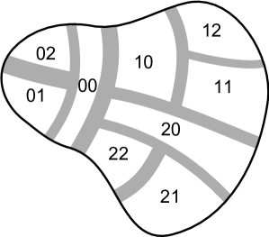
(c) 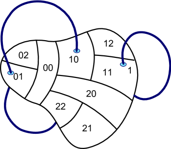 (d)
(d) 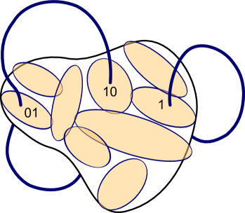
The problem we address here is sketched in figure 2; while a deterministic partition can, in principle, be made arbitrarily fine, in practice any noise will blur the boundaries and render the best possible partition finite. Thus our task is to determine the optimal attainable resolution of the state space of a given hyperbolic dynamical system, affected by a given weak noise. This we do by formulating the optimal partition hypothesis which we believe determines the best possible state space partition for a desired level of predictive precision. We know of no practical way of computing the ‘blurred’ partition boundaries of figure 2 (b). Instead, we propose to determine the optimal partition in terms of blurring of periodic point neighborhoods, as in figure 2 (d). As we demonstrate in sect. 5, our implementation requires determination of only a small set of solutions of the deterministic equations of motion.
Intuitively, the noise smears out the neighborhood of a periodic point, whose size is now determined by the interplay between the diffusive spreading parameterized Einstein (1905); Dekker and Kampen (1979); Gaspard et al. (1995) by a diffusion constant, and its exponentially shrinking deterministic neighborhood. If the noise is weak, the short-time dynamics is not altered significantly: short periodic orbits of the deterministic flow still coarsely partition the state space. As the periods of periodic orbits increase, the diffusion always wins, and successive refinements of a deterministic partition of the state space stop at the finest attainable partition, beyond which the diffusive smearing exceeds the size of any deterministic subpartition.
There is a considerable literature (reviewed here in remark 5.1) on interplay of noise and chaotic deterministic dynamics, and the closely related problem of limits on the validity of the semi-classical periodic orbit quantization. All of this literature implicitly assumes uniform hyperbolicity and seeks to define a single, globally averaged, diffusion induced average resolution (Heisenberg time, in the context of semi-classical quantization). However, the local diffusion rate differs from a trajectory to a trajectory, as different neighborhoods merge at different times, so there is no one single time beyond which noise takes over. Nonlinear dynamics interacts with noise in a nonlinear way, and methods for implementing the optimal partition for a given noise still need to be developed. This paper is an attempt in this direction. Here we follow and expand upon the Fokker-Planck approach to the ‘optimal partition hypothesis’ introduced in ref. Lippolis and Cvitanović (2010).
What is novel here is that we show how to compute the locally optimal partition, for a given dynamical system and given noise, in terms of local eigenfunctions of the forward-backward actions of the Fokker-Planck operator and its adjoint. This is much simpler than it sounds: the Lyapunov equation
(and its generalizations to periodic points of hyperbolic flows), determines , the size of local neighborhood, as balance of the noise variance and the linearized dynamics . The effort of going local brings a handsome reward: as the optimal partition is always finite, the dynamics on this ‘best possible of all partitions’ is encoded by a finite transition graph of finite memory, and the Fokker-Planck operator can be represented by a finite matrix. In addition, while the state space of a generic deterministic flow is an infinitely interwoven hierarchy of attracting, hyperbolic, elliptic and parabolic regions, the noisy dynamics erases any structures finer than the optimal partition, thus curing both the affliction of long-period attractors/elliptic islands with very small immediate basins of attraction/ellipticity, and the power-law correlation decays caused by marginally stable regions of state space.
The dynamical properties of high-dimensional flows are not just simple extensions of lower-dimensional dynamics, and a persuasive application of the Ruelle / Gutzwiller periodic orbit theory to high-dimensional dynamics would be an important advance. If such flow has only a few expanding directions, the above set of overlapping stochastic ‘cigars’ should provide an optimal, computable cover of the long-time chaotic attractor embedded in a state space of arbitrarily high dimension.
The requisite Langevin / Fokker-Planck description of noisy flows is reviewed in sect. 2. This discussion leans heavily on the deterministic dynamics and periodic orbit theory notation, summarized in appendix A. In sect. 3 we derive the formulas for the size of noise-induced neighborhoods of attractive fixed and periodic points, for maps and flows in arbitrary dimension. These formulas are known as Lyapunov equations, reviewed in appendix C. In order to understand the effect on noise on the hyperbolic, mixed expanding / contracting dynamics, we study the eigenfunctions of the discrete time Fokker-Planck operator in linear neighborhood of a fixed point of a noisy one-dimensional map in sect. 4, and show that the neighborhood along unstable directions is fixed by the evolution of a Gaussian density of trajectories under the action of the adjoint Fokker-Planck operator. The continuous time formulation of the same problem, known as the Ornstein-Uhlenbeck process, is reviewed in appendix B. Having defined the local neighborhood of every periodic point, we turn to the global partition problem. Previous attempts at state space partitioning are reviewed in remark 5.1. We formulate our optimal partition hypothesis in sect. 5: track the diffusive widths of unstable periodic orbits until they start to overlap. We test the approach by applying it to a 1-dimensional repeller, and in sect. 6, we assess the accuracy of our method by computing the escape rate and the Lyapunov exponent, discuss weak noise corrections, and compare the results with a discretization of the Fokker-Planck operator on a uniform mesh. In sect. 7 we address the problem of estimating the optimal partition of a non-hyperbolic map, where the linear approximation to the Fokker-Planck operator fails. The results are summarized and the open problems discussed in sect. 8.
2 Noisy trajectories and their densities
The literature on stochastic dynamical systems is vast, starting with the Laplace 1810 memoir Laplace (1810). The material reviewed in this section, sect. 4 and appendix B is standard van Kampen (1992); Risken (1996); Arnold (1974), but needed in order to set the notation for what is new here, the role that Fokker-Planck operators play in defining stochastic neighborhoods of periodic orbits. The key result derived here is the well known evolution law (14) for the covariance matrix of a linearly evolved Gaussian density,
To keep things simple we shall use only the discrete time dynamics in what follows, but we do discuss the continuous time formulation in appendix B, as our results apply both to the continuous and discrete time flows.
Consider a noisy discrete time dynamical system Kifer (1974); Feigenbaum and Hasslacher (1982); Boyarsky (1984)
| (1) |
where is a -dimensional state vector, and is its th component at time . In the Fokker-Planck description individual noisy trajectories are replaced by the evolution of the density of noisy trajectories, with the probability distribution of zero mean and covariance matrix (diffusion tensor) ,
| (2) |
where stands for ensemble average over many realizations of the noise.
The general case of a diffusion tensor which is a state space position dependent but time independent can be treated along the same lines. In this case the stochastic flow (1) is written as where is white noise, , is called the ‘diffusion matrix’, and the noise is referred to as ‘multiplicative’ (see Kuehn Kuehn (2011)).
The action of discrete one-time step Fokker-Planck operator on the density distribution at time ,
| (3) |
is centered on the deterministic step and smeared out diffusively by noise. Were diffusion uniform and isotropic, , the Fokker-Planck operator would be proportional to , i.e., the penalty for straying from the deterministic path is just a quadratic error function. The th iterate of is a -dimensional path integral over the intermediate noisy trajectory points,
| (4) |
where the Gaussian normalization factor in (3) is absorbed into intermediate integrations by defining
| (5) |
We shall also need to determine the effect of noise accumulated along the trajectory points preceding . As the noise is additive forward in time, one cannot simply invert the Fokker-Planck operator; instead, the past is described by the adjoint Fokker-Planck operator,
| (6) |
which transports a density concentrated around the point to a density concentrated around the previous point and adds noise to it. In the deterministic, vanishing noise limit this is the Koopman operator (LABEL:APPE3.14a).
The Fokker-Planck operator (3) is non-hermitian and non-unitary. For example, if the deterministic flow is contracting, the natural measure (the leading right eigenvector of the Fokker-Planck operator) will be concentrated and peaked, but then the corresponding left eigenvector has to be broad and flat, as backward in time the deterministic flow is expanding. We shall denote by the right eigenvectors of , and by its left eigenvectors, i.e., the right eigenvectors of the adjoint operator .
3 All nonlinear noise is local
Our first goal is to convince the reader that the diffusive dynamics of nonlinear flows is fundamentally different from Brownian motion, with the flow inducing a local, history dependent noise. In order to accomplish this, we go beyond the standard stochastic literature and generalize the notion of invariant deterministic recurrent solutions, such as fixed points and periodic orbits, to noisy flows. While a Langevin trajectory (1) cannot be periodic, in the Fokker-Planck formulation (4) a recurrent motion can be defined as one where a peaked distribution returns to the initial neighborhood after time . Recurrence so defined not only coincides with the classical notion of a recurrent orbit in the vanishing noise limit, but it also enables us to derive exact formulas for how this local, history dependent noise is to be computed.
As the function is a nonlinear function, in general the path integral (4) can only be evaluated numerically. In the vanishing noise limit the Gaussian kernel sharpens into the Dirac -function, and the Fokker-Planck operator reduces to the deterministic Perron-Frobenius operator (LABEL:TransOp1). For weak noise the Fokker-Planck operator can be evaluated perturbatively Cvitanović et al. (1998, 1999a, 1999b); Roncadelli (1995) as an asymptotic series in powers of the diffusion constant, centered on the deterministic trajectory. Here we retain only the linear term in this series, which has a particulary simple dynamics given by a covariance matrix evolution formula (see (14) and (22) below) that we now derive.
We shift local coordinates to the deterministic trajectory , , , centered coordinate frames , Taylor expand , and approximate the noisy map (1) by its linearization,
| (7) |
with the deterministic trajectory points at , and the one step Jacobian matrix (see appendix A). The corresponding linearized Fokker-Planck operator (3) is given in the local coordinates by
| (8) |
by the linearization (7) centered on the deterministic trajectory
| (9) |
The subscript ‘’ in distinguishes the local, linearized Fokker-Planck operator from the full operator (4).
The kernel of the linearized Fokker-Planck operator (9) is a Gaussian. As a convolution of a Gaussian with a Gaussian is again a Gaussian, we investigate the action of the linearized Fokker-Planck operator on a normalized, cigar-shaped Gaussian density distribution
| (10) |
and the action of the linearized adjoint Fokker-Planck operator on density
| (11) |
also centered on the deterministic trajectory, but with its own strictly positive covariance matrices , . Label ‘’ plays a double role, and stands both for the next, initial space partition and for the times the trajectory lands in these partitions (see appendix LABEL:DL:detPart). The linearized Fokker-Planck operator (9) maps the Gaussian into the Gaussian
| (12) |
one time step later. Likewise, linearizing the adjoint Fokker-Planck operator (6) around the trajectory point yields:
| (13) |
Completing the squares, integrating and substituting (10), respectively (11) we obtain the formula for covariance matrix evolution forward in time,
| (14) |
and in the adjoint case, the evolution of the is given by
| (15) |
The two covariance matrices differ, as the adjoint evolution is computed by going backwards along the trajectory. These covariance evolution rules are the basis of all that follows, except for the ‘flat-top’ of sect. 7.
Think of the initial covariance matrix (10) as an error matrix describing the precision of the initial state, a cigar-shaped probability distribution . In one time step this density is deterministically advected and deformed into density with covariance , and then the noise is added: the two kinds of independent uncertainties add up as sums of squares, hence the covariance evolution law (14), resulting in the Gaussian ellipsoid whose widths and orientation are given by the singular values and singular vectors (LABEL:SVD-j) of the covariance matrix. After time steps, the variance is built up from the deterministically propagated initial distribution, and the sum of noise kicks at intervening times, , also propagated deterministically.
The pleasant surprise is that the evaluation of this noise requires no Fokker-Planck PDE formalism. The width of a Gaussian packet centered on a trajectory is fully specified by a deterministic computation that is already a pre-computed byproduct of the periodic orbit computations; the deterministic orbit and its linear stability. We have attached label ‘’ to in (14) to account for the noise distributions that are inhomogeneous, state space dependent, but time independent multiplicative noise. As we shall show, in nonlinear dynamics the noise is never isotropic and/or homogeneous. For example, if the iterative system we are studying is obtained by Poincaré sections of a continuous time flow, the accumulated noise integrated over one Poincaré section return depends on the return trajectory segment, even when the infinitesimal time step noise (64) is homogenous.
Remark 3.1
Covariance evolution. In quantum mechanics the linearized evolution operator corresponding to the linearized Fokker-Planck operator (9) is known as the Van Vleck propagator, the basic block in the semi-classical periodic orbit quantization Gutzwiller (1990); Cvitanović et al. (2012). covariance matrix composition rule (14) or its continuous time version (83) is called ‘covariance evolution’ in ref. Tippett and Cohn (2001), for example, but it goes all the way back to Lyapunov’s 1892 thesis Lyapunov (1992), see appendix C. In the Kalman filter literature Kalman (1960); Abarbanel et al. (2009) it is called ‘prediction’.
3.1 The attractive, the repulsive and the noisy
For Browniam dynamics , with , we obtain , i.e., the variance of a Gaussian packet of noisy trajectories grows linearly in time, as expected for the Brownian diffusion. What happens for nontrivial, , dynamics? The formulas (14) and (15) are exact for finite numbers of time steps, but whether they have a long time limit depends on the stability of the deterministic trajectory.
Here we shall derive the limit for deterministic flows that are either contracting or expanding in all eigen-directions, with asymptotic stationary distributions concentrated either on fixed points or periodic points. We shall consider the general hyperbolic flows, where some of the eigen-directions are unstable, and other stable in another publication Cvitanović and Lippolis (2012). In this context the description in terms of periodic orbits is very useful; the neighborhood of a periodic point will be defined as the noise contracting neighborhood forward in time along contracting eigen-directions, backward in time along the unstable, expanding eigen-directions. The short cycles will be the most important ones, and only finite time, single cycle period calculations will be required.
If is contracting, with the multipliers in time steps the memory of the covariance of the starting density is forgotten at exponential rate , with iteration of (14) leading to a limit distribution:
| (16) |
For fixed and periodic points we can give an explicit formula for the covariance.
Consider a noisy map (1) with a deterministic fixed point at . In a neighborhood we approximate the map by its linearization (7) with the fixed point at , acting on a Gaussian density distribution (10), also centered on . The distribution is cigar-shaped ellipsoid, with eigenvectors of giving the orientation of various axes at time , see figure LABEL:f:repPart (b). If the fixed point is attractive, with all multipliers of strictly contracting, any compact initial measure (not only initial distributions of Gaussian form) converges under applications of (14) to the unique invariant natural measure whose covariance matrix satisfies the condition
| (17) |
For a repelling fixed point the condition (15) on the adjoint eigenvector yields
| (18) |
with a very different interpretation: as the Jacobian matrix has only expanding Floquet multipliers, the deterministic dynamics expands the fixed-point neighborhood exponentially, with no good notion of a local neighborhood in the large forward time limit. Instead, its past defines the neighborhood, with the covariance of the optimal distribution of points that can reach the fixed point in one time step, given the diffusion tensor .
These conditions are central to control theory, where the attracting fixed point condition (17) is called the Lyapunov equation (see appendix C), and are known respectively as controllability and observability Gramians, and there is much wisdom and open source code available to solve these (see remark LABEL:rem:LyapEq), as well as the more general hyperbolic equations. In order to develop some intuition about the types of solutions we shall encounter, we assume first, for illustrative purposes, that Jacobian matrix has distinct real contracting Floquet multipliers and right eigenvectors Construct from the column eigenvectors a similarity transformation
that diagonalizes , and its transpose Define and The fixed point condition (17) now takes form The matrix elements are so
| (19) |
and the attracting fixed point covariance matrix in the original coordinates is given by
| (20) |
For the adjoint case, the same algebra yields
| (21) |
for the matrix elements of , with the covariance matrix in the fixed coordinates again given by .
As (20) is not a similarity transformation, evaluation of the covariance matrix requires a numerical diagonalization, which yields the singular values and singular vectors (principal axes) of the equilibrium Gaussian ‘cigar’ (see appendix A). The singular vectors of this symmetric matrix have their own orientations, distinct from the left/right eigenvectors of the non-normal Jacobian matrix .
Remark 3.2
Hyperbolic flows. The methods to treat the cases where some of the eigen-directions are unstable, and other stable are implicit in the Oseledec Oseledec (1968) definition of Lyapunov exponents, the rigorous proof of existence of classical spectral (Fredholm) determinants by Rugh Rugh (1992), and the controllability and observability Gramians of control theory Zhou et al. (1999): the flow at a hyperbolic fixed point or cycle point can be locally factorized into stable and unstable directions, and for unstable directions one needs to study noise evolution in the past, by means of the adjoint operator (6).
3.2 In nonlinear world noise is never isotropic
Now that we have established the exact formulas (14), (15) for the extent of the noise-smeared out neighborhood of a fixed point, we turn to the problem of computing them for periodic orbits. An attractive feature of the deterministic periodic orbit theory is that certain properties of periodic orbits, such as their periods and Floquet multipliers, are intrinsic, independent of where they are measured along the the periodic orbit, and invariant under all smooth conjugacies, i.e., all smooth nonlinear coordinate transformations. Noise, however, is specified in a given coordinate system and breaks such invariances (for an exception, a canonically invariant noise, see Kurchan Cepas and Kurchan (1998)). Each cycle point has a different memory and differently distorted neighborhood, so we need to compute the Fokker-Planck eigenfunction at each cycle point .
The basic idea is simple: A periodic point of an -cycle is a fixed point of the th iterate of the map (1). Hence the formula (16) for accumulated noise, together the fixed point condition (17) also yields the natural measure covariance matrix at a periodic point on a periodic orbit ,
| (22) |
where
| (23) | |||||
is the noise accumulated per a single transversal of the periodic orbit, is the cycle Jacobian matrix (LABEL:perPointM) evaluated on the periodic point , and we have used the periodic orbit condition . Similarly, for the adjoint evolution the fixed point condition (18) generalizes to
| (24) |
where
| (25) | |||||
is the noise accumulated per a single transversal of the periodic orbit backward in time.
As there is no single coordinate frame in which different can be simultaneously diagonalized, the accumulated noise is never isotropic. So the lesson is that regardless of whether the external noise is isotropic or anisotropic, the nonlinear flow always renders the effective noise anisotropic and spatially inhomogeneous.
4 One-dimensional intuition
The very general, exact formulas that we have obtained so far (and so easily), valid in any dimension, might be elegant, but it is a bit hard to get one’s head around a formula such as the expression for the accumulated cycle noise (23). These results are easier to grasp by studying the effect of noise on 1-dimensional systems, such as the noisy linear map (7),
| (26) |
with the deterministic fixed point at , and additive white noise (2) with variance . The density of trajectories evolves by the action of the Fokker-Planck operator (3):
| (27) |
If a 1-dimensional noisy linear map (26) is contracting, any initial compact measure converges under applications of (27) to the unique invariant natural measure concentrated at the deterministic fixed point whose variance (10) is given by (17):
| (28) |
The variance (22) of a periodic point on an attractive -cycle is
| (29) |
where the accumulated noise per a cycle traversal (23) is given by
| (30) |
Variance (28) expresses a balance between contraction by and diffusive smearing by at each time step. For strongly contracting , the width is due to the noise only. As the width diverges: the trajectories are only weakly confined and diffuse by Brownian motion into a broad Gaussian.
Consider next the adjoint operator acting on a repelling noisy fixed point, . The stationary measure condition (18) yields
| (31) |
While the dominant feature of the attracting fixed point variance (28) was the diffusion strength , weakly modified by the contracting multiplier, for the unstable fixed point the behavior is dominated by the expanding multiplier ; the more unstable the fixed point, the smaller is the neighborhood one step in the past that can reach it.
The variance (24) of a periodic point on an unstable -cycle is
| (32) |
For an unstable cycle typically all derivatives along the cycle are expanding, , so the dominant term in (32) is the most recent one, . By contrast, forward in time (29) the leading estimate of variance of an attractive periodic point is . These leading estimates are not sensitive to the length of the periodic orbit, so all trajectories passing through a neighborhood of periodic point will have comparable variances.
4.1 Ornstein-Uhlenbeck spectrum
The variance (17) is stationary under the action of , and the corresponding Gaussian is thus an eigenfunction. Indeed, as we shall now show, for the linear flow (27) the entire eigenspectrum is available analytically, and as can always be brought to a diagonal, factorized form in its orthogonal frame, it suffices to understand the simplest case, the Ornstein-Uhlenbeck process (see appendix B.1) in one dimension. The linearized Fokker-Planck operator is a Gaussian, so it is natural to consider the set of Hermite polynomials, , , , , as candidates for its eigenfunctions. is an th-degree polynomial, orthogonal with respect to the Gaussian kernel
| (33) |
There are three cases to consider:
expanding case: The form of the left eigenfunction (31) suggests that we rescale and absorb the Gaussian kernel in (33) into left eigenfunctions , , ,
| (34) |
The right eigenfunctions are then
| (35) |
By construction the left, right eigenfunctions are orthonormal to each other:
| (36) |
One can verify Risken (1996) that for the fixed point , these are the right, left eigenfunctions of the adjoint Fokker-Planck operator (6), where the th eigenvalue is . Note that the Floquet multipliers are independent of the noise strength, so they are the same as for the deterministic Perron-Frobenius operator (LABEL:TransOp1).
marginal case: This is the pure diffusion limit, and the behavior is not exponential, but power-law. If the map is nonlinear, one needs to go to the first non-vanishing nonlinear order in Taylor expansion (LABEL:TaylExp) to reestablish the control Gaspard et al. (1995). This we do in sect. 7.
contracting case: In each iteration the map contracts the cloud of noisy trajectories by Floquet multiplier toward the fixed point, while the noise smears them out with variance . Now what was the left eigenfunction for the expanding case (34) is the peaked right eigenfunction of the Fokker-Planck operator, , , ,, with eigenvalues , , , Dekker and Kampen (1979); Gaspard et al. (1995)
| (37) |
where is the th Hermite polynomial, and follows from the prefactor in (34).
These discrete time results can be straightforwardly generalized to continuous time flows of sect. B, as well as to higher dimensions. So far we have used only the leading eigenfunctions (the natural measure), but in sect. 6 we shall see that knowing the whole spectrum in terms of Hermite polynomial is a powerful tool for the computation of weak-noise corrections.
Remark 4.1
Ornstein-Uhlenbeck process. The simplest example of a continuous time stochastic flow (63) is the Langevin flow (76) in one dimension. In this case, nothing is lost by considering discrete-time dynamics which is strictly equivalent to the continuous time Ornstein-Uhlenbeck process (77) discussed in appendix B.1.
5 Have no fear of globalization
We are now finally in position to address our challenge: Determine the finest possible partition for a given noise.
We shall explain our ‘the best possible of all partitions’ hypothesis by formulating it as an algorithm. For every unstable periodic point of a chaotic one-dimensional map, we calculate the corresponding width of the leading Gaussian eigenfunction of the local adjoint Fokker-Planck operator . Every periodic point is assigned a one-standard deviation neighborhood . We cover the state space with neighborhoods of orbit points of higher and higher period , and stop refining the local resolution whenever the adjacent neighborhoods, say of and , overlap in such a way that . As an illustration of the method, consider the chaotic repeller on the unit interval
| (38) |
with noise strength .
(a) 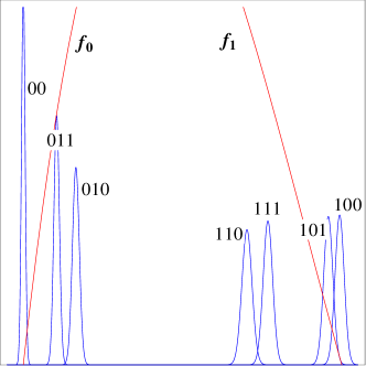 (b)
(b) 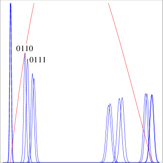
The map is plotted in figure 3 (a), together with the local eigenfunctions with variances given by (32). Each Gaussian is labeled by the branches visitation sequence of the corresponding deterministic periodic point (a symbolic dynamics, however, is not a prerequisite for implementing the method). Figure 3 (b) illustrates the overlapping of partition intervals: , overlap and so do all other neighborhoods of the period cycle points, except for and . We find that in this case the state space (the unit interval) can be resolved into 7 neighborhoods
| (39) |
It turns out that resolving further into and would not affect our estimates, as it would produce the same transition graph.

Once the finest possible partition is determined, a finite binary tree like the one in figure 4 is drawn: Evolution in time maps the optimal partition interval , , etc.. This is summarized in the transition graph in figure 5, which we will use to estimate the escape rate and the Lyapunov exponent of the repeller.
(a) 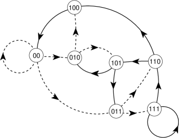 (b)
(b) 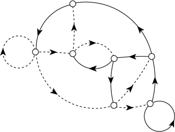 \thesource\thesourcesource: \thesourceChaosBook.org
Remark 5.1
A brief history of state space partitions. There is considerable prior literature that addresses various aspects of the ‘optimal partition’ problem. Before reviewing it, let us state what is novel about the optimal partition hypothesis formulated here: Our estimates of limiting resolution are local, differing from region to region, while all of the earlier limiting resolution estimates known to us are global, based on global averages such as Shannon entropy or quantum-mechanical ‘granularity’ of phase space. We know of no published algorithm that sets a limit to the resolution of a chaotic state space by studying the interplay of the noise with the local stretching/contracting directions of the deterministic dynamics, as we do here.
The engineering literature on optimal experimental design Fedorov (1972); Brown et al. (1985); Atkinson and Fedorov (1975); Fedorov and Khabarov (1986) employs criteria such as ‘-optimality,’ the maximization of the Shannon information content of parameter estimates. Purely statistical in nature, these methods have little bearing on the dynamical approach that we pursue here.
In 1983 Crutchfield and Packard Crutchfield and Packard (1983) were the first to study the problem of an optimal partition for a chaotic system in the presence of noise, and formulate a state space resolution criterion in terms of a globally averaged “attainable information.” The setting is the same that we assume here: the laws governing deterministic dynamics are given, and one studies the effects of noise (be it intrinsic, observational or numerical) on the dynamics. They define the most efficient symbolic encoding of the dynamics as the sequence of symbols that maximizes the metric entropy of the entire system, thus their resolution criterion is based on a global average. Once the maximum for a given number of symbols is found, they refine the partition until the entropy converges to some value. They formulate their resolution criterion in terms of attainable information, a limiting value for the probability to produce a certain sequence of symbols from the ensemble of all possible initial conditions. Once such limit is reached, no further refinements are possible.
Most of the dynamical systems literature deals with estimating partitions from observed data Daw et al. (2003). Tang and co-workers Tang et al. (1995) assume a noisy chaotic data set, but with the laws of dynamics assumed unknown. Their method is based on maximizing Shannon entropy and at the same time minimizing an error function with respect to the partition chosen. The same idea is used by Lehrman et al. Lehrman et al. (1997) to encode chaotic signals in higher dimensions, where they also detect correlations between different signals by computing their conditional entropy. For a review of symbolic analysis of experimental data up to 2001, see Daw, Finney and Tracy Daw et al. (2003).
Kennel and Buhl Kennel and Buhl (2003a, b); Buhl and Kennel (2005) estimate partitions for (high-dimensional) flows from noisy time-series data by minimizing a cost function which maximizes the correlation between distances in the state space and in the symbolic space, and indicates when to stop adjusting their partitions and therefore what the optimal partition is. In ref. Kennel and Buhl (2003a) their guiding principle for a good partition is that short sequences of consecutive symbols ought to localize the corresponding continuous state space point as well as possible. They embed symbol sequences into the unit square, and minimize the errors in localizing the corresponding state space points under candidate partitions. Holstein and Kantz Holstein and Kantz (2009) present an information-theoretic approach to determination of optimal Markov approximations from time series data based on balancing the modeling and the statistical errors in low-dimensional embedding spaces. Boland, Galla and McKane Boland et al. (2009) study the effects of intrinsic noise on a class of chemical reaction systems which in the deterministic limit approach a limit cycle in an oscillatory manner.
A related approach to the problem of the optimal resolution is that of the refinement of a transition matrix: given a chaotic, discrete-time dynamical system, the state space is partitioned, and the probabilities of points mapping between regions are estimated, so as to obtain a transition matrix, whose eigenvalues and eigenfunctions are then used to evaluate averages of observables defined on the chaotic set. The approach was first proposed in 1960 by Ulam Ulam (1960); Lasota and MacKey (1994), for deterministic dynamical systems. He used a uniform-mesh grid as partition, and conjectured that successive refinements of such coarse-grainings would provide a convergent sequence of finite-state Markov approximations to the Perron-Frobenius operator. Rechester and White Rechester and White (1991a, b) have proposed dynamics-based refinement strategies for constructing partitions for chaotic maps in one and two dimensions that would improve convergence of Ulam’s method.
Bollt et al. Bollt et al. (2008) subject a dynamical system to a small additive noise, define a finite Markov partition, and show that the Perron-Frobenius operator associated to the noisy system is represented by a finite-dimensional stochastic transition matrix. Their focus, however, is on approximating the natural measure of a deterministic dynamical system by the vanishing noise limit of a sequence of invariant measures of the noisy system.
In ref. Buhl and Kennel (2005) Kennel and Buhl approximate the distribution of the points in each symbolic region by a Gaussian with mean and variance ,
| (40) |
and estimate “code length” by the ad hoc Rissanen prior on , defined with no reference to dynamics, and thus morally unrelated to our periodic orbits based optimal partition.
Dellnitz and Junge Dellnitz and Junge (1998), Guder and Kreuzer Guder and Kreuzer (1999), Froyland Froyland (1998), and Keane et al. Keane et al. (1998) propose a variety of non-uniform refinement algorithms for such grids, reviewed in a monograph by Froyland Froyland (2001), who also treats their extension to random dynamical systems. In all cases, the ultimate threshold for every refinement is determined by the convergence of the spectrum of the transition matrix.
Theoretical investigations mostly focus on deterministic limits of stochastic models. The Sinai-Ruelle-Bowen Sinai (1972); Bowen (1975); Ruelle (1976) or natural measure (also called equilibrium measure, SRB measure, physical measure, invariant density, natural density, or natural invariant) is singled out amongst all invariant measures by its robustness to weak-noise perturbations, so there is considerable literature that studies it as the deterministic limit of a stochastic process.
6 Finite Fokker-Planck operator, and stochastic corrections
Next we show that the optimal partition enables us to replace Fokker-Planck PDEs by finite-dimensional matrices. The variance (32) is stationary under the action of , and the corresponding Gaussian is thus an eigenfunction. Indeed, as we showed in sect. 4.1, for the linearized flow the entire eigenspectrum is available analytically. For a periodic point , the th iterate of the linearization (9) is the discrete time version of the Ornstein-Uhlenbeck process, with left , , , respectively right , , mutually orthogonal eigenfunctions (34).
The number of resolved periodic points determines the dimensionality of the Fokker-Planck matrix. Partition (39) being the finest possible partition, the Fokker-Planck operator now acts as [] matrix with non-zero entries expanded in the Hermite basis,
| (41) | |||||
where , and is the deviation from the periodic point .
Periodic orbit theory (summarized in appendix A) expresses the long-time dynamical averages, such as Lyapunov exponents, escape rates, and correlations, in terms of the leading eigenvalues of the Fokker-Planck operator. In our optimal partition approach, is approximated by the finite-dimensional matrix , and its eigenvalues are determined from the zeros of , expanded as a polynomial in , with coefficients given by traces of powers of . As the trace of the th iterate of the Fokker-Planck operator is concentrated on periodic points , we evaluate the contribution of periodic orbit to by centering on the periodic orbit,
| (42) |
where are successive periodic points. To leading order in the noise variance , takes the deterministic value . The nonlinear diffusive effects in (41) can be accounted for Cvitanović et al. (1998) by the weak-noise Taylor series expansion around the periodic point ,
| (43) |
Such higher order corrections will be needed in what follows for a sufficiently accurate comparison of different methods.
(a) 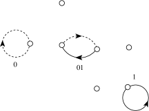 (b)
(b) 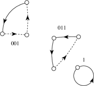 (c)
(c) 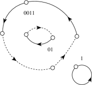
(d) 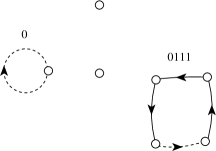 (e)
(e) 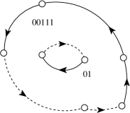 (f)
(f) 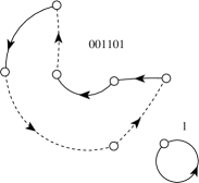
(g) 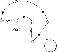 (h)
(h) 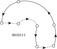 (i)
(i) 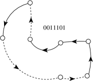
We illustrate the method by calculating the escape rate , where is the leading eigenvalue of Fokker-Planck operator , for the repeller plotted in figure 3. The spectral determinant can be read off the transition graph of figure 5 and its loop expansion in figure 6,
| (44) |
The polynomial coefficients are given by products of non-intersecting loops of the transition graph Cvitanović et al. (2012), with the escape rate given by the leading root of the polynomial. Twelve periodic orbits , , , , , , , , , , , up to period 7 (out of the 41 contributing to the noiseless, deterministic cycle expansion up to cycle period 7) suffice to fully determine the spectral determinant of the Fokker-Planck operator. In the evaluation of traces (42) we include stochastic corrections up to order (an order beyond the term kept in (43)). The escape rate of the repeller of figure 3 so computed is reported in figure 7.
Since our optimal partition algorithm is based on a sharp overlap criterion, small changes in noise strength can lead to transition graphs of different topologies, and it is not clear how to assess the accuracy of our finite Fokker-Planck matrix approximations. We make three different attempts, and compute the escape rate for: (a) an under-resolved partition, (b) several deterministic, over-resolved partitions, and (c) a direct numerical discretization of the Fokker-Planck operator.
(a) In the example at hand, the partition in terms of periodic points , , and is under-resolved; the corresponding escape rate is plotted in figure 7. (b) We calculate the escape rate by over-resolved periodic orbit expansions, in terms of all deterministic periodic orbits of the map up to a given period, with evaluated in terms of Fokker-Planck local traces (42), including stochastic corrections up to order . Figure 7 shows how the escape rate varies as we include all periodic orbits up to periods 2 through 8. Successive estimates of the escape rate appear to converge to a value different from the optimal partition estimate. (c) Finally, we discretize the Fokker-Planck operator by a piecewise-constant approximation on a uniform mesh on the unit interval Ulam (1960),
| (45) |
where is the th interval in equipartition of the unit interval into equal segments. Empirically, intervals suffice to compute the leading eigenvalue of the discretized matrix to four significant digits. This escape rate, figure 7, is consistent with the optimal partition estimate to three significant digits.
(a) 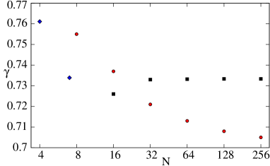 (b)
(b) 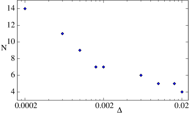
We estimate the escape rate of the repeller (38) for a range of values of the noise strength . The optimal partition method requires a different numbers of neighborhoods every time for different noise strengths. The results are illustrated by figure 7 (b) and 8, with the estimates of the optimal partition method within of those given by the uniform discretization of Fokker-Planck. One can also see from the same table that the escape rates calculated with and without higher order corrections to the matrix elements (41) are consistent within less than , meaning that the stochastic corrections (43) do not make a significant difference, compared to the effect of the optimal choice of the partition, and need not be taken into account in this example.
(a) 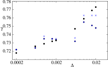 (b)
(b) 
The optimal partition estimate of the Lyapunov exponent is given by , where the cycle expansion average of an integrated observable Cvitanović et al. (2012)
| (46) | |||||
is the finite sum over cycles contributing to (44), and , the sum over the points of cycle , is the cycle Lyapunov exponent. On the other hand, we also use the discretization (45) to cross check our estimate: this way the Lyapunov exponent is evaluated as the average
| (47) |
where is the leading eigenfunction of (45), is the escape rate, and is the normalized repeller measure, . Figure 8 shows close agreement () between the Lyapunov exponent estimated using the average (46), where (no higher-order stochastic corrections), and the same quantity evaluated with (47), by the discretization method (45).
Remark 6.1
Weak noise corrections. The weak-noise corrections to the spectrum of evolution operators were first treated by Gaspard Gaspard (2002) for continuous-time systems, and in a triptych of articles Cvitanović et al. (1998, 1999a, 1999b) for discrete-time maps: they can be computed perturbatively to a remarkably high order Dettmann (2004) in the noise strength . However, as we have shown here, the eigenvalues of such operators offer no guidance to the ‘optimal partition’ problem; one needs to compute the eigenfunctions.
7 When the Gaussian approximation fails
The state space of a generic deterministic flow is an infinitely interwoven hierarchy of attracting, hyperbolic and marginal regions, with highly singular invariant measures. Noise has two types of effects. First, it feeds trajectories into state space regions that are deterministically either disconnected or transient (“noise induced escape,” “noise induced chaos”) and second, it smoothens out the natural measure. Here, we are mostly concerned with the latter. Intuitively, the noisy dynamics erases any structures finer than the optimal partition, thus -in principle- curing both the affliction of long-period attractors/elliptic islands with very small immediate basins of attraction/ellipticity, and the slow, power-law correlation decays induced by marginally stable regions of state space. So how does noise regularize nonhyperbolic dynamics?
As a relatively simple example, consider the skew Ulam map Artuso et al. (1990a), i.e., the cubic map (38) with the parameter . The critical point is the maximum of on the unit interval, with vanishing derivative . As this map sends the unit interval into itself, there is no escape, but due to the quadratic maximum the (deterministic) natural measure exhibits a spike near the critical value (see, for example, ref. Ruelle (2009) for a discussion). As explained in ref. Artuso et al. (1990a), a close passage to the critical point effectively replaces the accumulated Floquet multiplier by its square root. For example, for the skew Ulam map (38) -cycles whose itineraries are of form spend long time in the neighborhood of , and then pass close to . In the neighborhood of the Floquet multiplier gains a factor for each of the first iterations, and then experiences a strong, square root contraction during the close passage to the critical point , resulting in the Floquet multiplier , and a Lyapunov exponent that converges to , rather than that would be expected in a hyperbolic flow for a close passage to a fixed point . The same strong contraction is experienced by the noise accumulated along the trajectory prior to the passage by the critical point, rendering, for example, the period-doubling sequences more robust to noise than one would naïvely expect Crutchfield et al. (1981); Shraiman et al. (1981); Feigenbaum and Hasslacher (1982).
For the corresponding noisy map (1) the critical point is extended into the ‘flat top’ region where , and the linearized, Gaussian approximation (9) to the Fokker-Planck operator does not hold. Thus, we should first modify our choice of densities and neighborhoods, as the whole construction leading to the optimal partition algorithm was based on the Gaussian approximation.
The adjoint Fokker-Planck operator acts on a Gaussian density centered at , as in (10):
| (48) | |||||
Suppose the point around which we want to approximate the new density, is very close to the critical point, so that we can write
| (49) |
During a close passage to the critical point, the variance does not transform linearly, but as a square root:
| (50) |
We show in appendix D that in the next iteration the variance of the density transforms again like the variance of a Gaussian, up to order in the noise strength. By the same procedure, one can again assume the next preimage of the map is such that the linear approximation is valid, and transform the density (Eq. (89), appendix D) up to and obtain the same result for the variance, that is
| (51) |
which is again the evolution of the variances in the Gaussian approximation. In other words, the evolution of the variances goes back to be linear, to , although the densities transformed from the ‘quartic Gaussian’ (49) are no longer Gaussians.
The question is now how to modify the definition of neighborhoods given in sect. 5, in order to fit the new approximation. Looking for eigenfunctions of seems to be a rather difficult task to fulfill, given the functional forms (49) and (89) involved. Since we only care about the variances, we define instead the following map
| (52) |
, for the evolution of the densities, and take its periodic points as our new neighborhoods. In practice, one can compute these numerically, but we will not need orbits longer than length in our tests of the partition, therefore we can safely assume only one periodic point of to be close to the flat top, and obtain analytic expressions for the periodic points of (52):
| (53) |
with , is valid when the cycle starts and ends at a point close to the flat top. Otherwise, take the periodic point , that is the th preimage of the point . The corresponding periodic point variance has the form
| (54) |
both expressions (53) and (54) are approximate, as we further assumed , which is reasonable when , our range of investigation for the noise strength. As before, a neighborhood of width is assigned to each periodic point , and an optimal partition follows. However, due to the geometry of the map, such partitions as
| (55) |
can occur. In this example the regions and overlap, and the partition results in a transition graph with three loops (cycles) of length one, while we know that our map only admits two fixed points. In this case we decide to follow the deterministic symbolic dynamics and ignore the overlap.
Let us now test the method by estimating once again the escape rate of the noisy map (38). We note that the matrix elements
| (56) | |||||
, should be redefined in the neighborhood of the critical point of the map, where the Gaussian approximation to fails. We follow the approximation made in (49):
| (57) |
However, as decreases, it also reduces the quadratic term in the expansion of the exponential, so that the linear term must now be included in the matrix element:
| (58) |
(a) 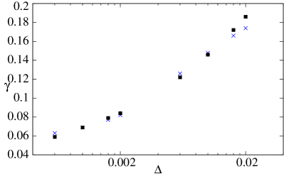 (b)
(b) 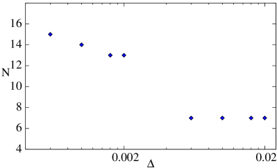
We find in our model that the periodic orbits we use in our expansion have ’s within the flat top, such that and , and therefore (57) better be replaced with (58) when . In order to know whether a cycle point is close enough to the flat top for the Gaussian approximation to fail, we recall that the matrix element (56) is the zeroth-order term of a series in , whose convergence can be probed by evaluating the higher order corrections (43): when the and corrections are of an order of magnitude comparable or bigger than the one of (56), we conclude that the Gaussian approximation fails and we use (57) or (58) instead. Everywhere else we use our usual matrix elements (56), without the higher-order corrections, as they are significantly larger than in the case of the repeller, and they are not accounted for by the optimal partition method, which is entirely based on a zeroth-order Gaussian approximation of the evolution operator. Like before, we tweak the noise strength within the range and compare the escape rate evaluated with the optimal partition method and with the uniform discretization (45). The results are illustrated in figure 9: the uniform discretization and the method of the optimal partition are consistent within a margin.
8 Summary and conclusions
Physicists tend to believe that with time Brownian motion leads to broadening of a noisy trajectory neighborhood. In nonlinear dynamics nothing of the sort happens; the noise broadening is balanced by non-linear stretching and contraction, and infinite length recurrent Langevin trajectories have finite noise widths, not widths that spread time. Here periodic orbits play special role: computable in finite time, they persist for for infinite time, and are thus natural objects to organize state space partitions around. On the other hand, computation of unstable periodic orbits in high-dimensional state spaces, such as Navier-Stokes, is at the border of what is currently feasible numerically Kawahara and Kida (2001); Cvitanović and Gibson (2010), and criteria to identify finite sets of the most important solutions are very much needed. Where are we to stop calculating orbits of a given hyperbolic flow? Intuitively, as we look at longer and longer periodic orbits, their deterministic neighborhoods shrink exponentially with time, while the variance of the noise-induced orbit smearing remains bounded; there has to be a turnover time, a time at which the noise-induced width overwhelms the exponentially shrinking deterministic dynamics, so that no better resolution is possible. Given a specified noise, we need to find, periodic orbit by periodic orbit, whether a further sub-partitioning is possible.
We have described here the optimal partition hypothesis, a method for partitioning the state space of a chaotic repeller in presence of weak Gaussian noise first introduced in ref. Lippolis and Cvitanović (2010). The key idea is that the width of the linearized adjoint Fokker-Planck operator eigenfunction computed on an unstable periodic point provides the scale beyond which no further local refinement of state space is feasible. This computation enables us to systematically determine the optimal partition, the finest state space resolution attainable for a given chaotic dynamical system and a given noise. Once the optimal partition is determined, we use the associated transition graph to describe the stochastic dynamics by a finite dimensional Fokker-Planck matrix. An expansion of the Fokker-Planck operator about periodic points was already introduced in refs. Cvitanović et al. (1998, 1999a, 1999b), with the stochastic trace formulas and determinants Cvitanović et al. (1998); Gaspard (2002) expressed as finite sums, truncated at orbit periods corresponding to the local turnover times. A novel aspect of the work presented here is its representation in terms of the Hermite basis (sect. B.1), eigenfunctions of the linearized Fokker-Planck operator (9), and the finite dimensional matrix representation of the Fokker-Planck operator.
It should be noted that our linearization of Fokker-Planck operators does not imply that the nonlinear dynamics is being modeled by a linear one. Our description is fully nonlinear, with periodic orbits providing the nonlinear backbone of chaotic dynamics, dressed up stochastically by Fokker-Planck operators local to each cycle. This is a stochastic cousin of Gutzwiller’s WKB approximation based semi-classical quantization Gutzwiller (1971) of classically chaotic systems, where in a parallel effort to utilize quantum-mechanical ‘graininess’ of the quantum phase space to terminate periodic orbit sums, Berry and Keating Berry and Keating (1990) have proposed inclusion of cycles of periods up to a single ‘Heisenberg time’. In light of the stochastic dynamics insights gained here, this proposal merits a reexamination - each neighborhood is likely to have its own Heisenberg time.
The work of Abarbanel et al. Abarbanel et al. (1991a, b, 2009); Quinn and Abarbanel (2009) suggest one type of important application beyond the low-dimensional Fokker-Planck calculations undertaken here. In data assimilation in weather prediction the convolution of noise variance and trajectory variance (14) is a step in the Kalman filter procedure. One could combine the state space charts of turbulent flows of ref. Gibson et al. (2008) (computed in the full 3-dimensional Navier-Stokes) with partial information obtained in experiments (typically a full 3-dimensional velocity field, fully resolved in time, but measured only on a 2-dimensional disk section across the pipe). The challenge is to match this measurement of the turbulent flow with a state space point in a -dimensional ODE representation, and then track the experimental observation to improve our theoretical prediction for the trajectory in the time ahead. That would be the absolutely best ‘weather prediction’ attainable for a turbulent pipe flow, limited by a combination of Lyapunov time and observational noise. In our parlance, the ‘optimal partition of state space.’
We have tested our optimal partition hypothesis by applying it to evaluation of the escape rates and the Lyapunov exponents of a repeller in presence of additive noise. In the setting numerical tests indicate that the ‘optimal partition’ method can be as accurate as the much finer grained direct numerical Fokker-Planck operator calculations. In higher dimensions (and especially in the extreme high dimensions required by fluid dynamics stimulations) such direct Fokker-Planck PDE integrations are not feasible, while the method proposed here is currently the only implementable approach.
The success of the optimal partition hypothesis in a one-dimensional setting is encouraging, and use of noise as a smoothing device that eliminates singularities and pathologies from clusterings of orbits is promising. However, higher-dimensional hyperbolic maps and flows, for which an effective optimal partition algorithm would be very useful, present new, as yet unexplored challenges of disentangling the subtle interactions between expanding, marginal and contracting directions; the method has not yet been tested in a high-dimensional hyperbolic setting. A limiting factor to applications of the periodic orbit theory to high-dimensional problems ranging from fluid flows to chemical reactions might be the lack of a good understanding of periodic orbits in more than three dimensions, of their stability properties, their organization and their impact on the dynamics.
In summary: Each periodic point owns a cigar, which for a high-dimensional dissipative flow is shaped along a handful of expanding and least-contracting directions. The remaining large (even infinite!) number of the strongly contracting directions is limited by the noise; the cigar always has the dimensionality of the full state space. Taken together, the set of overlapping cigars, or the optimal partition, weaves the carpet (of the full dimensionality of state space) which envelops the entire ‘inertial manifold’ explored by turbulent dynamics.
Acknowledgments.
We are grateful to D. Barkley, T. Bartsch, C.P. Dettmann, H. Fogedby, A. Grigo, A. Jackson, R. Mainieri, W.H. Mather, R. Metzler, E. Ott, S.A. Solla, N. Søndergaard, and G. Vattay for many stimulating discussions. Special thanks go to M. Robnik who made it possible to present this work at the 8th Maribor Summer School ‘Let’s Face Chaos through Nonlinear Dynamics’, which brought us together with T. Prosen, from whom we have learned that fixed points of the covariance evolution equations are the Lyapunov equations. P.C. thanks Glen P. Robinson, Jr. for support. D.L. was supported by NSF grant DMS-0807574 and G.P. Robinson, Jr..
Appendix A Periodic orbit theory, deterministic dynamics
We offer here a brief review of deterministic dynamics and periodic orbit theory. All of this is standard, but needed to set the notation used above. The reader might want to consult ref. Cvitanović et al. (2012) for further details.
Though the main applications we have in mind are to continuous flows, for purposes at hand it will suffice to consider discrete time dynamics obtained, for example, by reducing a continuous flow to mappings between successive Poincaré sections, as in figure LABEL:f:PoincSct. Consider dynamics induced by iterations of a -dimensional map where is the state space (or ‘phase space’) of the system under consideration. The discrete ‘time’ is then an integer, the number of applications of a map. We denote the th iterate of map by composition
| (59) |
The trajectory of is the finite set of points ,
| (60) |
traversed in time , and the orbit of is the subset of all points of that can be reached by iterations of . Here is a point in the -dimensional state space , and the subscript indicates time. While a trajectory depends on the initial point , an orbit is a set invariant under dynamics. The transformation of an infinitesimal neighborhood of an orbit point under the iteration of a map follows from Taylor expanding the iterated mapping at finite time . The linearized neighborhood is transported by the Jacobian matrix
| (61) |
( for Jacobian, or derivative notation is frequently employed in the literature.) The formula for the linearization of th iterate
| (62) |
in terms of unit time steps follows from the chain rule for functional composition,
We denote by the th eigenvalue or multiplier of the Jacobian matrix , and by
Appendix B Fokker-Planck operator, continuous time formulation
The material reviewed in this appendix is standard van Kampen (1992); Risken (1996); Arnold (1974), but needed in order to set the notation for what is new here, the role that Fokker-Planck operators play in defining stochastic neighborhoods of periodic orbits.
Consider a -dimensional stochastic flow
| (63) |
where the deterministic velocity field is called ‘drift’ in the stochastic literature, and is additive noise, uncorrelated in time. A way to make sense of is to first construct the corresponding probability distribution for additive noise at a short but finite time . In time the deterministic trajectory advances by . As is arbitrary, it is desirable that the diffusing cloud of noisy trajectories is given by a distribution that keeps its form as . This holds if the noise is Brownian, i.e., the probability that the trajectory reaches is given by a normalized Gaussian
| (64) |
Here the deviation of the noisy trajectory from the deterministic one, can be viewed either in terms of velocities (continuous time formulation), or finite time maps (discrete time formulation),
| (65) |
where
| (66) |
is a sequence of points along the noisy trajectory, separated by time increments , and the superfix T indicates a transpose. The probability distribution is characterized by zero mean and covariance matrix (diffusion tensor)
| (67) |
where stands for ensemble average over many realizations of the noise. For example, in one dimension the white noise for a pure diffusion process (no advection, ) is a normally distributed random variable, with standard normal (Gaussian) probability distribution function,
| (68) |
of mean , variance , and standard deviation , uncorrelated in time:
| (69) |
describes the diffusion at any time, including the integer time increments , and thus provides a bridge between the continuous and discrete time formulations of noisy evolution. We have set in (69) anticipating the discrete time formulation of sect. 2.
In physical problems the diffusion tensor is almost always anisotropic: for example, the original Langevin flow Chandrasekhar (1943) is a continuous time flow in {configuration, velocity} phase space, with white noise probability distribution modeling random Brownian force kicks applied only to the velocity variables . In this case one thinks of diffusion coefficient as temperature. For sake of simplicity we shall sometimes assume that diffusion in dimensions is uniform and isotropic, . The more general case of a tensor which is a state space position dependent but time independent can be treated along the same lines, as we do in (14). In this case the stochastic flow (63) is written as Doob (1942) is called ‘diffusion matrix,’ and the noise is referred to as ‘multiplicative.’
The distribution (64) describes how an initial density of particles concentrated in a Dirac delta function at spreads in time . In the Fokker-Planck description individual noisy trajectories are replaced by the evolution of the density of noisy trajectories. The finite time Fokker-Planck evolution of an initial density is obtained by a sequence of consecutive short-time steps (64)
| (70) |
where , and the Gaussian normalization factor in (64) is absorbed into intermediate integrations by defining as
| (71) | |||||
The stochastic flow (63) can now be understood as the continuous time, limit, with the velocity noise a Gaussian random variable of zero mean and covariance matrix
| (72) |
It is worth noting that the continuous time flow noise in (63) and (72) is dimensionally a velocity , while the discrete time noise in (64), (67) is dimensionally a length . The continuous time limit of (70), , defines formally the Fokker-Planck operator
| (73) |
as a stochastic path (or Wiener) integral Shraiman et al. (1981); Martin et al. (1973); Risken (1996) for a noisy flow, and the associated continuous time Fokker-Planck (or forward Kolmogorov) equation van Kampen (1992); Risken (1996); Øksendal (2003) describes the time evolution of a density of noisy trajectories (63),
| (74) |
The limit and the proper definition of are delicate issues Itô (1944); Stratonovich (1968); Arnold (1974); Fox (1978) of no import for the applications of stochasticity studied here.
In probabilist literature Berglund and Gentz (2005) the differential operator is called ‘Fokker-Planck operator;’ here we reserve the term exclusively for the finite time, ‘Green function’ integral operator (73). The exponent
| (75) |
can be interpreted as a cost function which penalizes deviation of the noisy trajectory from its deterministic prediction , or, in the continuous time limit, the deviation of the noisy trajectory tangent from the deterministic velocity . Its minimization is one of the most important tools of the optimal control theory Pontryagin et al. (1962); Bellman (1957), with velocity along a trial path varied with aim of minimizing its distance to the target .
The finite time step formulation (70) of the Fokker-Planck operator motivates the exposition of sect. 2, which starts by setting . In the linearized setting, the two formulations are fully equivalent.
Remark B.1
A brief history of noise. The cost function (75) appears to have been first introduced by Wiener as the exact solution for a purely diffusive Wiener-Lévy process in one dimension, see (68). Onsager and Machlup Onsager and Machlup (1953); Freidlin and Wentzel (1998) use it in their variational principle to study thermodynamic fluctuations in a neighborhood of single, linearly attractive equilibrium point (i.e., without any dynamics). The dynamical ‘action’ Lagrangian in the exponent of (73), and the associated symplectic Hamiltonian were first written down in 1970’s by Freidlin and Wentzell Freidlin and Wentzel (1998), whose formulation of the ‘large deviation principle’ was inspired by the Feynman quantum path integral Feynman and Hibbs (1965). Feynman, in turn, followed Dirac Dirac (1933) who was the first to discover that in the short-time limit the quantum propagator (imaginary time, quantum sibling of the Wiener stochastic distribution (68)) is exact. Gaspard Gaspard (2002) thus refers to the ‘pseudo-energy of the Onsager-Machlup-Freidlin-Wentzell scheme.’ M. Roncadelli Roncadelli (1995); Defendi and Roncadelli (1995) refers to the Fokker-Planck exponent in (73) as the ‘Wiener-Onsager-Machlup Lagrangian,’ constructs weak noise saddle-point expansion and writes transport equations for the higher order coefficients.
B.1 Ornstein-Uhlenbeck process
The variance (17) is stationary under the action of , and the corresponding Gaussian is thus an eigenfunction. Indeed, for the linearized flow the entire eigenspectrum is available analytically, and as can always be brought to a diagonal, factorized form in its orthogonal frame, it suffices to understand the simplest case, the Ornstein-Uhlenbeck process in one dimension. This simple example will enable us to show that the noisy measure along unstable directions is described by the eigenfunctions of the adjoint Fokker-Planck operator.
The simplest example of a stochastic flow (63) is the Langevin flow in one dimension,
| (76) |
with ‘drift’ linear in , and the single deterministic equilibrium solution . The associated Fokker-Planck equation (74) is known as the Ornstein-Uhlenbeck process Uhlenbeck and Ornstein (1930); Dekker and Kampen (1979); Gaspard et al. (1995); Wax (1954); Risken (1996):
| (77) |
(Here , Einstein diffusion constant.) One can think of this equation as the linearization of the Fokker-Planck equation (74) around an equilibrium point. For negative constant the spreading of noisy trajectories by random kicks is balanced by the linear damping term (linear drift) which contracts them toward zero. For this choice of , and this choice only, the Fokker-Planck equation can be rewritten as the Schrödinger equation for the quantum harmonic oscillator, with its well-known Hermite polynomial eigenfunctions Abramowitz and Stegun (1964); Takada et al. (2001) discussed here in sect. 4.1.
The key ideas are easier to illustrate by the noisy, strictly equivalent discrete-time dynamics of sect. 4.1, rather than by pondering the meaning of the stochastic differential equation (77).
Remark B.2
Quantum mechanical analogue. The relation between Ornstein-Uhlenbeck process and the Schrödinger equation for the quantum harmonic oscillator is much older than quantum mechanics: Laplace Laplace (1810) wrote down in 1810 what is now known as the Fokker-Planck equation and computed the Ornstein-Uhlenbeck process eigenfunctions Jacobsen (1997) in terms of Hermite polynomials (33). According to L Arnold Arnold (1974) review of the original literature, the derivations are much more delicate: the noise is colored rather than Dirac delta function in time. He refers only to the linear case (76) as the ‘Langevin equation’.
Appendix C Lyapunov equation
In his 1892 doctoral dissertation Lyapunov (1992) A. M. Lyapunov defined a dynamical flow to be “stable in the sense of Lyapunov” if the scalar Lyapunov function
computed on the state space of dynamical flow satisfies the ‘inflow’ condition
| (78) |
While there is no general method for constructing Lyapunov functions, for a linear -dimensional autonomous flow, the Lyapunov function can be taken quadratic,
| (79) |
and (78) takes form
Here is the transpose of the stability matrix , and is the shorthand for matrix being positive definite (or Hurwitz), i.e., having the entire eigenvalue spectrum, , in the right-hand half of the complex plane. Strict positivity guarantees that is invertible.
The Lyapunov differential equation for a time varying system is
| (80) |
For steady state, time invariant solutions , (80) becomes the Lyapunov matrix equation
| (81) |
The Lyapunov theorem Lyapunov (1992); Bellman (1960) states that a matrix has all its characteristic roots with real parts positive if, and only if, for any positive definite symmetric matrix , there exists a unique positive definite symmetric matrix that satisfies the continuous Lyapunov equation (81). The flow is then said to be asymptotically stable. In our application we are given a noise correlation matrix , and the theorem states the obvious: the stationary state with a covariance matrix exists provided that the stability matrix is stable, . We have to require strict stability, as would allow for a noncompact, Brownian diffusion along the marginal stability eigen-directions.
For a linear discrete-time system the quadratic Lyapunov function (79) must satisfy
leading to the discrete Lyapunov equation
| (82) |
Lyapunov theorem now states that there is a unique solution , provided the Jacobian matrix is a convergent matrix, i.e., a matrix whose eigenvalues (Floquet multipliers) are all less than unity in magnitude,
We note in passing that the effective diffusive width is easily recast from the discrete map formulation back into the infinitesimal time step form of appendix B:
| (83) |
where is the stability matrix. Expanding to linear order yields the differential version of the equilibrium condition (17)
| (84) |
(with the proviso that now is covariance matrix (72) for the velocity fluctuations). The condition (84) is well known Arnold (1974); Keizer (1987); Risken (1996) and widely used, for example, in the molecular and gene networks literature Paulsson (2004, 2005); Hornung and Barkai (2008); Bruggeman et al. (2009). In one dimension, (see (LABEL:stabExpon)), diffusion tensor , and the diffusive width is given by Arnold (1974)
| (85) |
a balance between the diffusive spreading and the deterministic contraction rate . If , the measure spreads out diffusively.
Appendix D Confluent hypergeometric functions and Laguerre polynomials
Let now transform this new density, around the next pre-image , as
| (87) |
where . Now change the variable , and write the density as a power series, so that the previous integral reads
| (88) |
We then group all the terms up to order and neglect and higher, and call
| (89) |
where (also sometimes called or in the literature) is a confluent hypergeometric function of the first kind Gradshteyn and Ryzhik (1965), which can be expressed as
| (90) |
We now want to evaluate the variance of the density (89)
| (91) |
It is useful to know, when computing the denominator of (91), that
| (92) |
so that
| (93) | |||||
in the last identity we used the definition of and (50).
Next we derive (90), which expresses the a confluent hypergeometric function in terms of an exponential and a Laguerre polynomial. Start with the identity Gradshteyn and Ryzhik (1965):
| (94) |
in particular, the hypergeometric function in (89) becomes
| (95) |
A confluent hypergeometric function can be written in terms of a Laguerre polynomial Gradshteyn and Ryzhik (1965):
| (96) |
Thus, in our case
| (97) |
and
| (98) |
References
- van Kampen (1992) N. G. van Kampen, Stochastic Processes in Physics and Chemistry, North-Holland, Amsterdam, 1992.
- Lasota and MacKey (1994) A. Lasota, and M. MacKey, Chaos, Fractals, and Noise; Stochastic Aspects of Dynamics, Springer, Berlin, 1994.
- Risken (1996) H. Risken, The Fokker-Planck Equation, Springer, New York, 1996.
- Gaspard (2002) P. Gaspard, J. Stat. Phys. 106, 57 (2002).
- Fogedby (2005) H. C. Fogedby, Phys. Rev. Lett. 94, 195702 (2005).
- Fogedby (2006) H. C. Fogedby, Phys. Rev. E 73, 031104 (2006).
- Lippolis and Cvitanović (2010) D. Lippolis, and P. Cvitanović, Phys. Rev. Lett. 104, 014101 (2010), arXiv:0902.4269.
- Ruelle (1978) D. Ruelle, Statistical Mechanics, Thermodynamic Formalism, Addison-Wesley, Reading, MA, 1978.
- Cvitanović (1988) P. Cvitanović, Phys. Rev. Lett. 61, 2729 (1988).
- Einstein (1905) A. Einstein, Ann. Physik 17, 549 (1905).
- Dekker and Kampen (1979) H. Dekker, and N. G. V. Kampen, Phys. Lett. A 73, 374–376 (1979).
- Gaspard et al. (1995) P. Gaspard, G. Nicolis, A. Provata, and S. Tasaki, Phys. Rev. E 51, 74 (1995).
- Laplace (1810) P. S. Laplace, Mem. Acad. Sci. (I), XI, Section V. pp. 375–387 (1810).
- Arnold (1974) L. Arnold, Stochastic Differential Equations: Theory and Applications, Wiley, New York, 1974.
- Kifer (1974) Y. Kifer, Math. USSR-Izv. 8, 1083–1107 (1974).
- Feigenbaum and Hasslacher (1982) M. J. Feigenbaum, and B. Hasslacher, Phys. Rev. Lett. 49, 605–609 (1982).
- Boyarsky (1984) A. Boyarsky, Physica D 11, 130–146 (1984).
- Kuehn (2011) C. Kuehn, Deterministic continutation of stochastic metastable equilibria via Lyapunov equations and ellipsoids (2011), arXiv:1106.3479.
- Cvitanović et al. (1998) P. Cvitanović, C. P. Dettmann, R. Mainieri, and G. Vattay, J. Stat. Phys. 93, 981 (1998), arXiv:chao-dyn/9807034.
- Cvitanović et al. (1999a) P. Cvitanović, C. P. Dettmann, R. Mainieri, and G. Vattay, Nonlinearity 12, 939 (1999a), arXiv:chao-dyn/9811003.
- Cvitanović et al. (1999b) P. Cvitanović, N. Søndergaard, G. Palla, G. Vattay, and C. P. Dettmann, Phys. Rev. E 60, 3936 (1999b), arXiv:chao-dyn/9904027.
- Roncadelli (1995) M. Roncadelli, Phys. Rev. E 52, 4661 (1995).
- Gutzwiller (1990) M. Gutzwiller, Chaos in Classical and Quantum Mechanics, Springer, Berlin, 1990.
- Cvitanović et al. (2012) P. Cvitanović, R. Artuso, R. Mainieri, G. Tanner, and G. Vattay, Chaos: Classical and Quantum, Niels Bohr Institute, Copenhagen, 2012, ChaosBook.org.
- Tippett and Cohn (2001) M. K. Tippett, and S. E. Cohn, Nonlinear Processes in Geophysics 8, 331–340 (2001).
- Lyapunov (1992) A. M. Lyapunov, Int. J. Control 55, 531–534 (1992).
- Kalman (1960) R. E. Kalman, Trans. ASME – J. Basic Engineering 82, 35–45 (1960).
- Abarbanel et al. (2009) H. D. I. Abarbanel, D. R. Creveling, R. Farsian, and M. Kostuk, SIAM J. Appl. Math. 8, 1341–1381 (2009).
- Cvitanović and Lippolis (2012) P. Cvitanović, and D. Lippolis, Optimal resolution of the state space of a chaotic flow in presence of noise (2012), in preparation.
- Oseledec (1968) V. I. Oseledec, Trans. Moscow Math. Soc. 19, 197–221 (1968).
- Rugh (1992) H. H. Rugh, Nonlinearity 5, 1237 (1992).
- Zhou et al. (1999) K. Zhou, G. Salomon, and E. Wu, Int. J. Robust and Nonlin. Contr. 9, 183–198 (1999).
- Cepas and Kurchan (1998) O. Cepas, and J. Kurchan, European Physical Journal B 2, 221 (1998), arXiv:cond-mat/9706296.
- Fedorov (1972) V. Fedorov, Theory of Optimal Experiments, Academic Press, New York, 1972.
- Brown et al. (1985) L. D. Brown, I. Olkin, J. Sacks, and H. P. Wynn, editors, Jack Carl Kiefer Collected Papers, Springer, Berlin, 1985, vol. III, chap. Design of Experiments, p. 718.
- Atkinson and Fedorov (1975) A. C. Atkinson, and V. V. Fedorov, Biometrika 62, 57–70 (1975).
- Fedorov and Khabarov (1986) V. Fedorov, and V. Khabarov, Biometrika 73, 183–190 (1986).
- Crutchfield and Packard (1983) J. P. Crutchfield, and N. H. Packard, Physica D 7, 201–223 (1983).
- Daw et al. (2003) C. S. Daw, C. E. A. Finney, and E. R. Tracy, Rev. Sci. Instrum. 74, 915–930 (2003).
- Tang et al. (1995) X. Z. Tang, E. R. Tracy, A. D. Boozer, A. deBrauw, and R. Brown, Phys. Rev. E 51, 3871–3889 (1995).
- Lehrman et al. (1997) M. Lehrman, A. B. Rechester, and R. B. White, Phys. Rev. Lett. 78, 54 (1997).
- Kennel and Buhl (2003a) M. B. Kennel, and M. Buhl, Phys. Rev. Lett. 91, 084102 (2003a), arXiv:nlin/0304054.
- Kennel and Buhl (2003b) M. B. Kennel, and M. Buhl, “Estimating good discrete partitions from observed data: symbolic false nearest neighbors,” in Experimental Chaos: Seventh Experimental Chaos Conference, edited by L. Kočarev, T. L. Carroll, B. J. Gluckman, S. Boccaletti, and J. Kurths, Am. Inst. of Phys., Melville, New York, 2003b, pp. 380–380.
- Buhl and Kennel (2005) M. Buhl, and M. B. Kennel, Phys. Rev. E 71, 046213 (2005).
- Holstein and Kantz (2009) D. Holstein, and H. Kantz, Phys. Rev. E 79, 056202 (2009), arXiv:0808.1513.
- Boland et al. (2009) R. P. Boland, T. Galla, and A. J. McKane, Limit cycles, complex Floquet multipliers and intrinsic noise (2009), arXiv:0903.5248.
- Ulam (1960) S. M. Ulam, A Collection of Mathematical Problems, Interscience Publishers, New York, 1960.
- Rechester and White (1991a) A. B. Rechester, and R. B. White, Phys. Lett. A 156, 419–424 (1991a).
- Rechester and White (1991b) A. B. Rechester, and R. B. White, Phys. Lett. A 158, 51–56 (1991b).
- Bollt et al. (2008) E. Bollt, P. Góra, A. Ostruszka, and K. Życzkowski, SIAM J. Applied Dynam. Systems 7, 341–360 (2008), arXiv:nlin/0605017.
- Hunt and Ott (1996) B. R. Hunt, and E. Ott, Phys. Rev. Lett. 76, 2254 (1996).
- Yang et al. (2000) T.-H. Yang, B. R. Hunt, and E. Ott, Phys. Rev. E 62, 1950 (2000).
- Dellnitz and Junge (1998) M. Dellnitz, and O. Junge, Computing and Visualization in Science 1, 63–68 (1998).
- Guder and Kreuzer (1999) R. Guder, and E. Kreuzer, Nonlinear Dynamics 20, 21–32 (1999).
- Froyland (1998) G. Froyland, Nonlinear Analysis, Theory, Methods and Applications 32, 831–860 (1998).
- Keane et al. (1998) M. Keane, R. Murray, and L.-S. Young, Nonlinearity 11, 27–46 (1998).
- Froyland (2001) G. Froyland, “Extracting dynamical behaviour via Markov models,” in Nonlinear Dynamics and Statistics: Proc. Newton Inst., Cambridge 1998, edited by A. Mees, Birkhäuser, Boston, 2001, pp. 281–321.
- Graham and Tél (1984a) R. Graham, and T. Tél, J. Stat. Phys. 35, 729 (1984a).
- Graham and Tél (1984b) R. Graham, and T. Tél, Phys. Rev. Lett. 52, 9–12 (1984b).
- Graham et al. (1985) R. Graham, D. Roekaerts, and T. Tél, Phys. Rev. A 31, 3364 (1985).
- Graham and Tél (1986) R. Graham, and T. Tél, Phys. Rev. A 33, 1322–1337 (1986).
- Graham and Tél (1990) R. Graham, and T. Tél, Phys. Rev. A 42, 4661–4677 (1990).
- Graham et al. (1991) R. Graham, A. Hamm, and T. Tél, Phys. Rev. Lett. 66, 3089–3092 (1991).
- Hamm and Graham (1992) A. Hamm, and R. Graham, J. Stat. Phys. 66, 689–725 (1992).
- Sinai (1972) Y. G. Sinai, Russian Math. Surveys 166, 21 (1972).
- Bowen (1975) R. Bowen, Equilibrium States and the Ergodic Theory of Anosov Diffeomorphisms, Springer, Berlin, 1975.
- Ruelle (1976) D. Ruelle, Invent. Math. 34, 231 (1976).
- Uhlenbeck and Ornstein (1930) G. E. Uhlenbeck, and L. S. Ornstein, Phys. Rev. 36, 823–841 (1930).
- Dettmann (2004) C. P. Dettmann, Physica D 187, 214–222 (2004).
- Artuso et al. (1990a) R. Artuso, E. Aurell, and P. Cvitanović, Nonlinearity 3, 361 (1990a).
- Ruelle (2009) D. Ruelle, Nonlinearity 22, 855–870 (2009), arXiv:arXiv.org:0901.0484.
- Crutchfield et al. (1981) J. R. Crutchfield, M. Nauenberg, and J. Rudnick, Phys. Rev. Lett. 46, 933 (1981).
- Shraiman et al. (1981) B. Shraiman, C. E. Wayne, and P. C. Martin, Phys. Rev. Lett. 46, 935–939 (1981).
- Kawahara and Kida (2001) G. Kawahara, and S. Kida, J. Fluid Mech. 449, 291–300 (2001).
- Cvitanović and Gibson (2010) P. Cvitanović, and J. F. Gibson, Geometry of turbulence in wall-bounded shear flows: Periodic orbits (2010), in S. I. Abarzhi and K. R. Sreenivasan, eds., Turbulent Mixing and Beyond, Proc. 2nd Int. Conf. ICTP, Trieste,
- Gutzwiller (1971) M. C. Gutzwiller, J. Math. Phys. 12, 343–358 (1971).
- Berry and Keating (1990) M. V. Berry, and J. P. Keating, J. Phys. A 23, 4839–4849 (1990).
- Abarbanel et al. (1991a) H. D. I. Abarbanel, R. Brown, and M. B. Kennel, Int. J. Mod. Phys. B 5, 1347–1375 (1991a).
- Abarbanel et al. (1991b) H. D. I. Abarbanel, R. Brown, and M. B. Kennel, J. Nonlinear Sci. 1, 175–199 (1991b).
- Quinn and Abarbanel (2009) J. C. Quinn, and H. D. I. Abarbanel, Quart. J. Royal Meteor. Soc. 136, 19 (2009), arXiv:0912.1581.
- Gibson et al. (2008) J. F. Gibson, J. Halcrow, and P. Cvitanović, J. Fluid Mech. 611, 107–130 (2008), arXiv:0705.3957.
- Gaspard (1997) P. Gaspard, Chaos, Scattering and Statistical Mechanics, Cambridge Univ. Press, Cambridge, 1997.
- Levnajić and Mezić (2008) Z. Levnajić, and I. Mezić, Ergodic theory and visualization I: Visualization of ergodic partition and invariant sets (2008), arXiv:0805.4221.
- Rowley et al. (2009) C. W. Rowley, I. Mezić, S. Bagheri, P. Schlatter, and D. S. Henningson, J. Fluid Mech. 641, 115 (2009).
- Artuso et al. (2012) R. Artuso, H. H. Rugh, and P. Cvitanović (2012), chapter “Why does it work?”, in ref. Cvitanović et al. (2012).
- Cvitanović and Eckhardt (1991) P. Cvitanović, and B. Eckhardt, J. Phys. A 24, L237 (1991).
- Artuso et al. (1990b) R. Artuso, E. Aurell, and P. Cvitanović, Nonlinearity 3, 325–359 (1990b).
- Chandrasekhar (1943) S. Chandrasekhar, Rev. Mod. Phys. 15, 1 (1943).
- Doob (1942) J. L. Doob, Ann. Math. 43, 351–369 (1942).
- Martin et al. (1973) P. C. Martin, E. D. Siggia, and H. A. Rose, Phys. Rev. A 8, 423 (1973).
- Øksendal (2003) B. Øksendal, Stochastic Differential Equations, Springer, New York, 2003.
- Itô (1944) K. Itô, Proc. Imp. Acad. Tokyo 20, 519–524 (1944).
- Stratonovich (1968) R. L. Stratonovich, Conditional Markov Processes and Their Application to the Theory of Control, Elsevier, New York, 1968.
- Fox (1978) R. F. Fox, Phys. Rep. 48, 179–283 (1978).
- Berglund and Gentz (2005) N. Berglund, and B. Gentz, Noise-Induced Phenomena in Slow-Fast Dynamical Systems: A Sample-Paths Approach, Springer, Berlin, 2005.
- Pontryagin et al. (1962) L. S. Pontryagin, V. Boltyanskii, R. Gamkrelidge, and E. Mishenko, Mathematical Theory of Optimal Processes, Interscience Publishers, New York, 1962.
- Bellman (1957) R. Bellman, Dynamic Programming, Princeton Univ. Press, Princeton, 1957.
- Onsager and Machlup (1953) L. Onsager, and S. Machlup, Phys. Rev. 91, 1505, 1512 (1953).
- Freidlin and Wentzel (1998) M. I. Freidlin, and A. D. Wentzel, Random Perturbations of Dynamical Systems, Springer, Berlin, 1998.
- Feynman and Hibbs (1965) R. Feynman, and A. Hibbs, Quantum Mechanics and Path Integrals, McGraw-Hill Book Co., New York, 1965.
- Dirac (1933) P. A. M. Dirac, Phys. Z. Sowjetunion 3, 64–72 (1933).
- Defendi and Roncadelli (1995) A. Defendi, and M. Roncadelli, J. Phys. A 28, L515–L520 (1995).
- Wax (1954) E. Wax, Selected Papers on Noise and Stochastic Processes, Dover, New York, 1954.
- Abramowitz and Stegun (1964) M. Abramowitz, and I. A. Stegun, editors, Handbook of Mathematical Functions, Dover, New York, 1964.
- Takada et al. (2001) H. Takada, Y. Kitaoka, and Y. Shimizua, Forma 16, 17–46 (2001).
- Jacobsen (1997) M. Jacobsen, Bernoulli 2, 271–286 (1997).
- Gradshteyn and Ryzhik (1965) I. S. Gradshteyn, and I. M. Ryzhik, Table of Integrals. Series, and Products, Academic Press, New York, 1965.
- Bellman (1960) R. Bellman, Introduction to Matrix Analysis, McGrew-Hill, New York, 1960.
- Keizer (1987) J. Keizer, Statistical Thermodynamics of Nonequilibrium Processes, Springer, Berlin, 1987.
- Paulsson (2004) J. Paulsson, Nature 427, 415–418 (2004).
- Paulsson (2005) J. Paulsson, Phys. Life Rev. 2, 157–175 (2005).
- Hornung and Barkai (2008) G. Hornung, and N. Barkai, PloS Computational Biology 4, e80055 (2008).
- Bruggeman et al. (2009) F. J. Bruggeman, N. Blüthgen, and H. V. Westerhoff, PloS Computational Biology 5, e1000506 (2009).
- Lancaster and Tismenetsky (1985) P. Lancaster, and M. Tismenetsky, The Theory of Matrices, Academic Press, New York, 1985.
- Taussky (1961) O. Taussky, J. SIAM 9, 640–643 (1961).
- Ostrowski and Schneider (1962) A. Ostrowski, and H. Schneider, J. Math. Anal. Appl. 4, 72–84 (1962).
- Carlson and Schneider (1962) D. Carlson, and H. Schneider, Bull. Amer. Math. Soc. 68, 479–484 (1962).
- Antoulas and Sorensen (2001) A. C. Antoulas, and D. C. Sorensen, Linear Algebra and its Applications 326, 137–150 (2001).
- Bartels and Stewart (1972) R. H. Bartels, and G. W. Stewart, Comm. ACM 15, 820–826 (1972).
- Kitagawa (1977) G. Kitagawa, Int. J. Control 25, 745–753 (1977).
- Golub et al. (1979) G. Golub, S. Nash, and C. Van Loan, IEEE Trans. Auto. Contr. 24, 909–913 (1979).
- Datta and Hong (2003) K. Datta, and Y. Hong, IEEE Trans. Auto. Contr. 48, 2223–2228 (2003).
- Bryson and Ho (1975) A. E. Bryson, and Y. C. Ho, Applied Optimal Control, Hemisphere Publ., 1975.
- Barraud (1977) A. Y. Barraud, IEEE Trans. Auto. Contr. 22, 883–885 (1977).
- Hammarling (1982) S. J. Hammarling, IMA J. Num. Anal. 2, 303–325 (1982).
- Higham (1988) N. J. Higham, A.C.M. Trans. Math. Soft. 14, 381–396 (1988).
- Penzl (1998) T. Penzl, Advances in Comp. Math. 8, 33–48 (1998).
- Meinsma (1995) G. Meinsma, Systems and Control Letters 25, 237–242 (1995).
- Packard et al. (1980) N. H. Packard, J. P. Crutchfield, J. D. Farmer, and R. S. Shaw, Phys. Rev. Lett. 45, 712–716 (1980).
- Goldhirsch et al. (1987) I. Goldhirsch, P. L. Sulem, and S. A. Orszag, Physica D 27, 311–337 (1987).
- Trevisan and Pancotti (1998) A. Trevisan, and F. Pancotti, J. Atmos. Sci. 55, 390 (1998).
- Wolfe and Samelson (2007) C. L. Wolfe, and R. M. Samelson, Tellus A 59, 355–366 (2007).