A Posteriori Error Analysis of Component Mode Synthesis for the Frequency Response Problem
Abstract
We consider the frequency response problem and derive a posteriori error estimates for the discrete error in a reduced finite element model obtained using the component mode synthesis (CMS) method. We provide estimates in a linear quantity of interest and the energy norm. The estimates reflect to what degree each CMS subspace influence the overall error in the reduced solution. This enables automatic error control through adaptive algorithms that determine suitable dimensions of each subspace. We illustrate the theoretical results by including several numerical examples.
Keywords: Component mode synthesis; model reduction; reduced order modeling; a posteriori error estimation; frequency response problem.
1 Introduction
Due to the large scale of finite element models of complex structures, it may be necessary to use reduced finite element models with much fewer degrees of freedom when performing frequency response analysis of a structure over a large range of frequencies. Having control over the reduction error in the approximation is then highly important. In this paper we derive a posteriori error estimates for the discrete error in the reduced solution to the frequency response problem obtained using component mode synthesis (CMS) [6, 7, 11, 4, 5].
The results in this paper complement the a posteriori analysis developed in [13] where CMS was applied to an elliptic model problem, and the a posteriori analysis in [14], where the elliptic eigenvalue problem was considered. Similar techniques are used and results obtained here as in the previous two publications. The frequency response problem does however require an explicit treatment due to the indefinite nature of the problem. We further present a new adaptive strategy suitable for frequency sweep analysis.
Other work on error analysis for CMS class methods include results by Bourquin who considered the elliptic eigenvalue problem and derived a priori bounds for the error in eigenvalues and eigenmodes [4, 5]; and results by Yang, Gao, Bai, Li, Lee, Husbands, and Ng [19] for the automated multilevel substructuring method [3], who derived a criterion for mode truncation; together with results by Elssel and Voss [8] who showed that the same criterion guarantees control of the error in the smallest eigenvalue in the reduced problem.
Previous work on frequency response analysis based on CMS include that by Bennighof and Kaplan [2], who developed an iterative method in which the response is split into two components, one component near resonance and one component representing the remainder of the response. The near resonant component is captured using approximate global eigenmodes, and the remainder of the response using substructure modes and iteration. A similar method was also proposed by Ko and Bai [15]. Error estimates for these methods have, to the author’s knowledge, not yet been developed.
Research on duality based a posteriori error estimation and adaptive refinement strategies in finite element modeling has been ongoing since the 1990’s. For a general introduction to the subject in context of finite element analysis we point the reader to [1, 10, 9], and the references therein. We also refer to [12, 16, 17, 18] for results that we feel are especially relevant in context of structural mechanics.
The remainder of this paper is organized as follows. In Section 2 we provide some prerequisite material and present the frequency response problem in linear elasticity; in Section 3 we give an account of the Craig-Bampton CMS in a variational setting; in Section 4 we derive an a posteriori error estimates for the error in the displacements in the reduced model measured in the energy norm; in Section 5 we demonstrate our results in several numerical examples; and in Section 6 we summarize our findings.
2 The Frequency Response Problem
Let be a bounded domain in , , , with boundary , where , let be a subdivision of into, for instance, triangles or tetrahedra , and let be the space of continuous, piecewise th order vector polynomials on defined by , where is the space of th order polynomials on element . Let further be the bounded, coercive bilinear form on defined by , where , let denote the inner product on , and let be the bounded linear form on given by , where is a body force, and is a traction force.
The finite element frequency response problem reads: find such that
| (2.1) |
Given a basis in , the following matrix form of (2.1) is obtained:
| (2.2) |
where is the stiffness matrix, is the mass matrix, is a damping matrix, assumed to be on the form , , , i.e. Rayleigh damping, and is the load vector. The vector of coefficients of is denoted by .
3 Component Mode Synthesis
Let be a partition of into connected subdomains , such that each , for some subset . Let the interface between the subdomains be denoted by . An -orthogonal decomposition
| (3.1) |
of associated with and may be constructed by letting , , and by letting
| (3.2) |
where denotes the trace space of associated with , and denotes the energy minimizing extension of a function to . That is, is defined by the problem: find , such that
| (3.3) | ||||
| (3.4) |
A basis in each subspace , , assumed to be of dimension , is obtained from the discrete eigenvalue problems: find for , such that
| (3.5) |
A reduced subspace , where is a multi-index, may be defined by letting
| (3.6) |
where
| (3.7) |
3.1 The Reduced Problem
Introducing the subspace in the model we get the following reduced problem: find such that
| (3.8) |
Collecting the coefficients of the reduced basis functions columnwise in the matrix , the matrix form of (3.8) reads
| (3.9) |
where
| (3.10) | ||||
| (3.11) | ||||
| (3.12) | ||||
| (3.13) |
Next, we turn to error estimation and derive a posteriori error estimates for the discrete error in the reduced problem.
4 A Posteriori Error Analysis
4.1 Preliminaries
We begin by remarking that for the error holds the Galerkin orthogonality property
| (4.1) |
obtained by subtracting (3.8) from the finite element formulation (2.1).
We further state the following notation, first introduced in [13]. Here and below , , denote Ritz projectors, that is, the projector defined by
| (4.2) |
and , denotes decomposition, such that
| (4.3) |
The operators , , denote series expansion in , such that
| (4.4) |
and the operator , similarly denotes expansion in the space , such that
| (4.5) |
We further let , , denote the discrete subspace residuals defined for by
| (4.6) |
We note here that the discrete residual is defined by
| (4.7) |
and that the projection of onto is given by
| (4.8) |
Hence, , and
| (4.9) |
Finally, for we define the operators , , by
| (4.10) |
where the , , are given by (3.5). We summarize some properties of in the following lemma whose proof is straight forward, and may be found in e.g [13].
Lemma 1.
For , , as defined in (4.10), the following properties hold:
| (4.11) | ||||||
| (4.12) | ||||||
| (4.13) |
4.2 A Posteriori Estimate in a Quantity of Interest
First we show a straight forward a posteriori error estimate for the discrete error in a quantity of interest defined by a linear functional. The quantity of interest may for instance be the mean stress on a part of the boundary, or the displacements near a point of interest.
Let therefore , , be a linear functional on , and let the goal of solving (3.8) be to accurately approximate . We introduce the dual problem: find , such that
| (4.14) |
Choosing in (4.14), the error may then be written
| (4.15) | ||||
| (4.16) | ||||
| (4.17) |
using (4.9), and using the triangle inequality, the estimate
| (4.18) |
immediately follows.
Now, using that is an orthonormal basis in , we have for the residual and the Ritz projection , respectively
| (4.19) | ||||
| (4.20) |
Thus,
| (4.21) |
Remark 1.
The accuracy in the reduced model of course depends on the dimensions of the subspaces , . Looking at the estimate (4.18), each term
| (4.22) |
accounts for the contribution to the error caused by truncating the basis in , . The may then be used as a decision basis in an adaptive algorithm that automatically refines the subspaces contributing the most to the error .
Remark 2.
To obtain , we need the residual and the dual solution . The coefficient vector of the residual is given by the equation
| (4.23) |
and the dual problem on matrix form reads
| (4.24) |
The coefficient vector of is given by the equation
| (4.25) |
where is a matrix containing the coefficients of a basis in in its columns. In the case of the modal basis , we then have , where is diagonal, and we obtain
| (4.26) | ||||
| (4.27) | ||||
| (4.28) | ||||
| (4.29) |
where we have used that is orthogonal to in the last equality, and introduced , which we assume contains the coefficients of the eigenmodes , together with the diagonal matrix containing the corresponding eigenvalues.
In practice the dual problem is approximately solved, for instance using a slightly larger reduced space , where , and , , compared to what is used in the primal problem. Similarly, in the Ritz projections of the dual solution onto the subspaces, approximations may be used. Due to orthogonality it is then sufficient to project onto the spaces , .
4.3 An Energy Norm Estimate
The following a posteriori error estimate in the energy norm holds.
Theorem 1.
Let and satisfy (2.1) and (3.8), respectively. Then the following a posteriori estimate holds for the energy norm of the discrete error in the approximation:
| (4.30) |
where and respectively, are defined by
| (4.31) | ||||
| (4.32) |
and is a stability factor, depending on the finite element eigenvalues and the frequency , defined by
| (4.33) |
where .
The terms and are given in matrix form by
| (4.34) | |||
| (4.35) |
Proof.
Introducing this dual split in (4.15), using the Galerkin orthogonality property (4.1) to subtract , we obtain
| (4.38) | ||||
| (4.39) | ||||
| (4.40) | ||||
| (4.41) | ||||
| (4.42) | ||||
| (4.43) | ||||
| (4.44) | ||||
| (4.45) |
We choose in the dual problem (4.14), which gives . Using property (4.13) in Lemma 1 together with the Cauchy-Schwarz inequality on the sums in (4.38), we then have
| (4.46) | ||||
Using that the decomposition of is -orthogonal, we have
| (4.47) |
from Parseval’s identity. It furthermore holds that
| (4.48) |
cf. e.g. [13].
Combining the above results, we arrive at
| (4.49) | ||||
| (4.50) |
We now turn to the question of stability of the dual solutions , . Beginning with in (4.36) we have
| (4.51) | ||||
| (4.52) |
and hence . Next, the solution to (4.37) is given by the Fourier expansion
| (4.53) |
where , , is a basis of elastic eigenmodes in , and . Using that , for , , we then have
| (4.54) | ||||
| (4.55) | ||||
| (4.56) |
and this completes the proof. ∎
Remark 3.
In Theorem 1, we may estimate further using Young’s inequality, to obtain the subspace indicators
| (4.57) |
which reflect to what degree modal truncation in each subspace influence the energy norm of the error in the reduced solution.
Using these indicators we may design adaptive algorithms that automatically determines suitable refinement levels in the individual subspaces. Such algorithms are outlined in Section 5, along with the different numerical examples.
Remark 4.
The matrix form of equation (4.7) for the subspace residual reads
| (4.58) |
In the case of the modal basis, , and
| (4.59) | ||||
| (4.60) | ||||
| (4.61) | ||||
The subspace residuals may similarly to the Ritz projections of the dual solution be approximately computed. For instance using the subspaces , , or mass lumping techniques.
Remark 5.
In practical application we cannot evaluate exactly as it depends on the finite element eigenvalues which in general are unknown and an approximation of must be used. Such an approximation may be obtained using a reduced model of the eigenvalue problem.
5 Numerical Examples
In this section we apply the above developed theory in three numerical examples. In the first example we describe and apply an adaptive algorithm based on the estimate (4.18) in a single load case; in the second example we describe and apply an algorithm based on (4.30) in a single load case: and in the third example we describe and apply an adaptive algorithm based on (4.30) for the computation of a series of responses when varies over a given range.
In all three examples we consider the domain seen in Figure 1. The domain is partitioned into subdomains , , interfacing at . We assume that the boundary is clamped at and stress free elsewhere. The reference finite element model is piecewise linear, defined on a triangular mesh containing approximately 7000 elements. The material constants are and , and the parameters and in the Rayleigh damping are chosen as .
Example 1.
We consider the single load case where , , and , with . We assume that the goal of the computation is to control the absolute error in the functional , where , and is the nodal interpolation operator on . This roughly amounts to accurately computing the displacements in the direction near the point . We use an adaptive algorithm of the form outlined in Algorithm 1.
Remark 6.
We use the following adaptive strategy: compute the normalized subspace indicators by . With the objective of adding a maximum of NMODES eigenmodes in a maximum of NITS iterations, add
| (5.1) |
modes in subspace , each iteration.
Choosing the parameters and in the adaptive strategy (5.1), the objective of the computation may be viewed as computing the output in as accurately as possible using approximately 200 DOF distributed over the course of 10 iterations. Using such an objective is motivated by considerations regarding available precomputed basis functions and computational resources.
We start the algorithm with the subspace dimensions . Each iteration we compute an approximate dual solution using eigenmodes in each dual subspace basis.
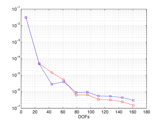
In Table 1 we see the subspace dimensions evolving as the adaptive algorithm proceeds, and in Figures 2, we see the corresponding absolute error together with the estimated error as the adaptation proceeds.
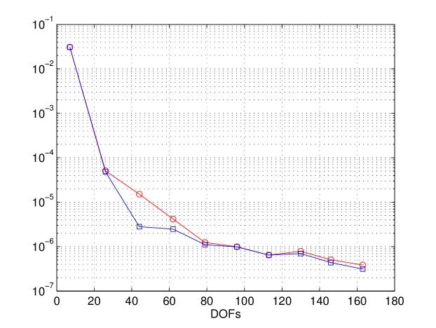
For comparison we have also run the algorithm using an exact dual solution . The resulting subspace dimensions are displayed in Table 2, and the error and estimate can be seen in Figure 3. We see that the adaptation is similar in both cases, and that the estimate with approximate dual is accurate, although a slight underestimate is introduced after the fourth iteration. The underestimation may be alleviated by refining the dual more aggressively during adaptation.
| iter. | |||||||
|---|---|---|---|---|---|---|---|
| 2 | 20 | 1 | 1 | 1 | 1 | 1 | 1 |
| 4 | 20 | 5 | 13 | 10 | 2 | 2 | 9 |
| 6 | 26 | 19 | 14 | 14 | 5 | 8 | 9 |
| 8 | 37 | 29 | 18 | 15 | 9 | 10 | 10 |
| 10 | 41 | 36 | 23 | 15 | 12 | 12 | 22 |
| iter. | |||||||
|---|---|---|---|---|---|---|---|
| 2 | 20 | 1 | 1 | 1 | 1 | 1 | 1 |
| 4 | 20 | 6 | 13 | 10 | 2 | 2 | 9 |
| 6 | 26 | 20 | 15 | 14 | 3 | 9 | 9 |
| 8 | 33 | 30 | 20 | 16 | 8 | 9 | 14 |
| 10 | 35 | 39 | 24 | 24 | 8 | 10 | 23 |
Example 2.
Next, we consider the load case , with , , and , with . In this example we aim to control the energy norm of the error as efficiently we can. We use an adaptive algorithm of the form outlined in Algorithm 2. Again we use the adaptive strategy (5.1) with the parameters and , and we start the algorithm with subspace dimensions . The stability factor is approximated using the eigenvalues from the reduced eigenvalue problem: find , such that
| (5.2) |
We remark that although the size of the stability factor is not crucial for the guiding of the adaptive algorithm in this example, having a reasonable estimate is however important for quantitative error estimation.
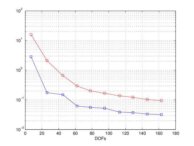
In Table 3 we see the subspace dimensions as the adaptation proceeds, and the corresponding error and estimate can be seen in Figure 4. From the table we see that the subspaces are refined symmetrically as should be expected from the given load. We see in the figure that the estimate provides an accurate bound on the error.
| iter. | |||||||
|---|---|---|---|---|---|---|---|
| 2 | 20 | 1 | 1 | 1 | 1 | 1 | 1 |
| 4 | 20 | 5 | 8 | 8 | 1 | 1 | 19 |
| 6 | 20 | 11 | 9 | 9 | 1 | 1 | 44 |
| 8 | 20 | 15 | 11 | 11 | 2 | 2 | 68 |
| 10 | 20 | 18 | 13 | 13 | 3 | 3 | 93 |
Example 3.
In this example we’re interested in computing the frequency response for a set of load cases. We let the goal of the computation be to control the relative error measured in energy norm for each load case, and we assume that the following estimate
| (5.3) |
holds approximately.
An adaptive algorithm designed to handle this setting is outlined in Algorithm 3. The algorithm utilizes that if a basis has been adaptively constructed for a given , that basis is likely well suited for the case as well, when is small and that the load pattern has not changed significantly. The algorithm refines the subspaces contributing to the error and coarsens the subspaces that do not in order to keep the dimension of the reduced subspace as small as it can.
Remark 7.
In Algorithm 3 we use a refinement strategy based on the following reasoning: begin by choosing a tolerance TOL, and let the objective for each load case be to refine the model such that the estimated relative error is the same as this tolerance, that is . Squaring both sides, we obtain
| (5.4) |
Assuming that each subspace should contribute equally to the error, so that
| (5.5) |
we have that each indicator should fulfill
| (5.6) |
By studying the difference
| (5.7) |
we obtain a subspace indicator , that is positive if refinement is required and negative if coarsening is required. By normalizing each indicator, we obtain a rough measure of how much each subspace should be refined or coarsened for (5.5) to hold true.
Hence, let , and choose , where is the number of precomputed eigenmodes for the th subspace. Then, if , add consecutive eigenmodes are to the th basis subject to , and if , remove the last modes from the th basis, subject to .
Further, if for some load case and subspace it holds that , and , , and , we consider the load case non resolvable given the current tolerance and maximum number of modes , and we let the algorithm continues to the next load case.
We let the load cases in the example be defined by , with , and constant, chosen as in Example 1. The parameters in the adaptive strategy outlined in Remark 7 are chosen as , , and , where the number of precomputed eigenmodes are , , . As in Example 2, we solve the reduced eigenvalue problem (5.2) for a sufficiently large set of eigenvalues needed to approximate the stability factor .
We start the algorithm with the subspace dimensions . The algorithm terminates after requiring a total of 59 refinement iterations in order to satisfy the error tolerance in each of the 30 load cases.
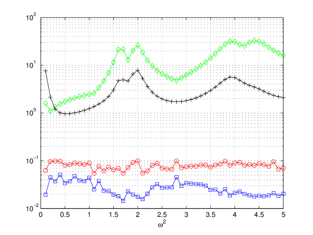
In Figure 5 we have plotted the energy norm of the solutions, relative errors, estimated relative errors, and stability factors, for each of the computed load cases. We see that overall the error is estimated to a high degree of accuracy, and we see that the estimate is close to the desired tolerance TOL=0.1, in every load case. The stability factor is large near , due to proximity of eigenvalues at and . Since the norm of the solution increases when approaching these values, the relative error decreases, however, leading to less accuracy in the estimated error. This reflects the fact that error estimation is more difficult near resonance frequencies.
In Table 4 we have displayed the obtained subspace dimensions and total dimension, the number of required iterations, and the efficiency index , for each load case in the range . We see that typically only one or two iterations is required for each load case, except in a few cases.
| DOFs | its | |||||||||
|---|---|---|---|---|---|---|---|---|---|---|
| 0.1 | 9 | 1 | 1 | 6 | 1 | 1 | 1 | 20 | 2 | 3.2035 |
| 0.2 | 9 | 1 | 1 | 39 | 1 | 1 | 2 | 54 | 3 | 2.0838 |
| 0.3 | 12 | 1 | 1 | 62 | 1 | 1 | 3 | 82 | 2 | 2.5641 |
| 0.4 | 14 | 1 | 1 | 120 | 1 | 1 | 2 | 108 | 5 | 2.3731 |
| 0.5 | 13 | 1 | 2 | 130 | 1 | 1 | 5 | 142 | 1 | 1.7461 |
| 0.6 | 15 | 1 | 1 | 157 | 1 | 1 | 3 | 154 | 3 | 2.2068 |
| 0.7 | 13 | 1 | 3 | 165 | 1 | 1 | 1 | 160 | 1 | 1.8104 |
| 0.8 | 12 | 1 | 1 | 172 | 1 | 1 | 5 | 173 | 1 | 1.8084 |
| 0.9 | 15 | 1 | 1 | 182 | 1 | 1 | 4 | 179 | 1 | 1.8141 |
| 1.0 | 13 | 1 | 4 | 187 | 1 | 1 | 1 | 188 | 1 | 2.2675 |
| 1.1 | 14 | 3 | 4 | 191 | 1 | 1 | 3 | 198 | 2 | 2.2362 |
| 1.2 | 11 | 9 | 5 | 193 | 1 | 1 | 4 | 206 | 2 | 2.0555 |
| 1.3 | 12 | 4 | 8 | 192 | 1 | 1 | 6 | 201 | 1 | 2.3509 |
| 1.4 | 14 | 6 | 2 | 190 | 1 | 1 | 5 | 213 | 2 | 2.7570 |
| 1.5 | 13 | 11 | 3 | 186 | 1 | 1 | 10 | 208 | 2 | 2.9929 |
| 1.6 | 14 | 15 | 4 | 178 | 1 | 1 | 14 | 223 | 4 | 3.7636 |
| 1.7 | 13 | 18 | 12 | 172 | 1 | 1 | 7 | 209 | 1 | 4.5314 |
| 1.8 | 11 | 18 | 8 | 168 | 1 | 1 | 3 | 203 | 1 | 3.1486 |
| 1.9 | 12 | 14 | 3 | 162 | 1 | 1 | 17 | 203 | 2 | 4.4424 |
| 2.0 | 10 | 13 | 13 | 159 | 1 | 1 | 14 | 205 | 2 | 4.3318 |
| 2.1 | 16 | 14 | 10 | 156 | 1 | 1 | 11 | 189 | 1 | 4.3043 |
| 2.2 | 13 | 13 | 5 | 152 | 1 | 1 | 6 | 181 | 1 | 3.0109 |
| 2.3 | 11 | 10 | 16 | 147 | 1 | 1 | 4 | 179 | 2 | 2.6907 |
| 2.4 | 11 | 9 | 7 | 143 | 1 | 1 | 13 | 175 | 1 | 2.5683 |
| 2.5 | 12 | 9 | 16 | 142 | 1 | 1 | 5 | 169 | 2 | 2.5769 |
| 2.6 | 15 | 9 | 8 | 142 | 1 | 1 | 7 | 174 | 2 | 2.4149 |
| 2.7 | 14 | 9 | 12 | 145 | 1 | 1 | 9 | 172 | 1 | 2.5297 |
| 2.8 | 11 | 9 | 7 | 147 | 1 | 1 | 4 | 175 | 1 | 2.3162 |
| 2.9 | 12 | 9 | 15 | 149 | 1 | 1 | 9 | 186 | 3 | 2.3814 |
| 3.0 | 19 | 10 | 7 | 151 | 1 | 1 | 3 | 176 | 1 | 2.5042 |
6 Summary and Outlook
We have presented an a posteriori error analysis for reduced finite element models of the frequency response problem in linear elasticity constructed using component mode synthesis. We have derived estimates for the error in the displacements measured in a linear goal functional, as well as for the error measured in the energy norm. The estimate reflects to what degree each CMS subspace influence the error in the reduced solution allowing the design of adaptive algorithms that automatically determines suitable subspace dimensions. We have demonstrated our results in several numerical examples. The numerical results follow the theoretical predictions to a high degree of accuracy. The future of this research concerns its application in real world three dimensional examples.
7 Acknowledgments
This research is supported by SKF and the Industrial Graduate School at Umeå University.
References
- [1] W. Bangerth and R. Rannacher, Adaptive finite element methods for differential equations, Lectures in Mathematics, Birkhäuser, 2003.
- [2] J. K. Bennighof and M. F. Kaplan, Frequency sweep analysis using multi-level substructuring, global modes and iteration, Proceedings of 39th AIAA/ASME/ASCE/-AHS Structures, Structural Dynamics and Materials Conference, Citeseer, 1998.
- [3] J. K. Bennighof and R. B. Lehoucq, An automated multilevel substructuring method for eigenspace computation in linear elastodynamics, SIAM Journal on Scientific Computing 25 (2004), no. 6, 2084–2106.
- [4] F. Bourquin, Analysis and comparison of several component mode synthesis methods on one dimensional domains, Numerische Mathematik 58 (1990), no. 1, 11–33.
- [5] , Component mode synthesis and eigenvalues of second order operators: Discretization and algorithm, Mathematical Modelling and Numerical Analysis (1992), no. 26, 385–423.
- [6] R. R. Craig and M. C. C. Bampton, Coupling of substructures for dynamic analysis, AIAA Journal (1968), no. 6, 1313–1321.
- [7] R. R. Craig and Chang C. J., “Substructure Coupling for Dynamic Analysis and Testing”, Nasa Contract Report CR-278 1 (1977).
- [8] K. Elssel and H. Voss, An a priori bound for automated multilevel substructuring, SIAM Journal on Matrix Analysis and Applications 28 (2007), no. 2, 386–397.
- [9] K. Eriksson, D. Estep, P. Hansbo, and C. Johnson, Introduction to adaptive methods for differential equations, Acta Numerica (1995), no. 4, 105–158.
- [10] M. B. Giles and E. Süli, Adjoint methods for PDEs: a posteriori error analysis and postprocessing by duality, Acta Numerica 11 (2003), 145–236.
- [11] W. C. Hurty, Dynamic analysis of structural systems using component modes, AIAA Journal (1965), no. 4, 678–685.
- [12] S. Irimie and P. Bouillard, A residual a posteriori error estimator for the finite element solution of the Helmholtz equation, Computer Methods in Applied Mechanics and Engineering 190 (2001), no. 31, 4027–4042.
- [13] H. Jakobsson, F. Bengzon, and M. G. Larson, Adaptive Component Mode Synthesis in Linear Elasticity, International Journal for Numerical Methods in Engineering 86 (2011), 829–844.
- [14] H. Jakobsson and M. G. Larson, A Posteriori Error Analysis of Component Mode Synthesis for the Elliptic Eigenvalue Problem, Computer Methods in Applied Mechanics and Engineering 200 (2011), 2840–2847.
- [15] J. H. Ko and Z. Bai, High-frequency response analysis via algebraic substructuring, International Journal for Numerical Methods in Engineering 76 (2008), 295–313.
- [16] M. G. Larson, A posteriori and a priori error analysis for finite element approximations of self-adjoint elliptic eigenvalue problems, SIAM Journal on Numerical Analysis 38 (2001), no. 2, 608–625.
- [17] J. T. Oden, S. Prudhomme, and L. Demkowicz, A posteriori error estimation for acoustic wave propagation problems, Archives of Computational Methods in Engineering 12 (2005), no. 4, 343–389.
- [18] R. Rannacher and F. T. Suttmeier, A posteriori error control and mesh adaptation for FE models in elasticity and elasto-plasticity, Studies in Applied Mechanics (1998), 275–292.
- [19] C. Yang, W. Gao, Z. Bai, X. S. Li, L. Q. Lee, P. Husbands, and E. Ng, An Algebraic Substructuring Method for Large-Scale Eigenvalue Calculation, SIAM Journal on Scientific Computing 27 (2005), 873.