Two properties of volume growth entropy
in Hilbert geometry

Abstract.

The aim of this paper is to provide two examples in Hilbert geometry which show that volume growth entropy is not always a limit on the one hand, and that it may vanish for a non-polygonal domain in the plane on the other hand.

1. Introduction

A Hilbert domain in $\mathbf{R}^{\!m\!}$ is a metric space $(\mathcal{C},d_{\mathcal{C}{}_{\!}})$, where $\mathcal{C}$ is an open bounded convex set in $\mathbf{R}^{\!m\!}$ and $d_{\mathcal{C}{}_{\!}}$ is the distance function on $\mathcal{C}$ — called the Hilbert metric — defined as follows.

Given two distinct points $p$ and $q$ in $\mathcal{C}$, let $a$ and $b$ be the intersection points of the straight line defined by $p$ and $q$ with $\partial\mathcal{C}$ so that $p=(1-s)a+sb$ and $q=(1-t)a+tb$ with $0<s<t<1$. Then

$$d_{\mathcal{C}{}_{\!}}(p,q)\ \mbox{\raisebox{0.366pt}{$:$}\!$=$}\ \frac{1}{2}\ln{\![a,p,q,b]}~{},$$

where

$$[a,p,q,b]\ \mbox{\raisebox{0.366pt}{$:$}\!$=$}\ \frac{1-s}{s}\!\times\!\frac{t}{1-t}\ >\ 1$$

is the cross ratio of the $4$-tuple of ordered collinear points $(a,p,q,b)$ (see Figure 1).
We complete the definition by setting $d_{\mathcal{C}{}_{\!}}(p,q)\ \mbox{\raisebox{0.366pt}{$:$}\!$=$}\ 0$ for $p=q$.

Figure 1. The Hilbert metric $d_{\mathcal{C}{}_{\!}}$

The metric space $(\mathcal{C},d_{\mathcal{C}{}_{\!}})$ thus obtained is a complete non-compact geodesic metric space whose topology is the one induced by the canonical topology of $\mathbf{R}^{\!m\!}$ and in which the affine open segments joining two points of the boundary $\partial\mathcal{C}$ are geodesic lines. It is to be mentioned here that in general the affine segment between two points in $\mathcal{C}$ may not be the unique geodesic joining these points (for example, if $\mathcal{C}$ is a square). Nevertheless, this uniqueness holds whenever $\mathcal{C}$ is strictly convex.

Moreover, the distance function $d_{\mathcal{C}{}_{\!}}$ is associated with the Finsler metric $F_{{}_{\!}\mathcal{C}{}_{\!}}$ on $\mathcal{C}$ given, for any $p\in\mathcal{C}$ and any $v\in T_{\!p}\mathcal{C}\equiv\mathbf{R}^{\!m\!}$ (the tangent vector space to $\mathcal{C}{}_{\!}$ at $p$), by

$$F_{{}_{\!}\mathcal{C}{}_{\!}}(p,v)\ \mbox{\raisebox{0.366pt}{$:$}\!$=$}\ \frac{1}{2}\!\left(\frac{1}{t^{-}}+\frac{1}{t^{+}}\right)\quad\mbox{for}\quad v\ \neq\ 0~{},$$

where $t^{-\!}=t_{\mathcal{C}}^{-\!}(p,v)$ and $t^{+\!}=t_{\mathcal{C}}^{+\!}(p,v)$ are the unique positive numbers satisfying $p-t^{-}v\in\partial\mathcal{C}$ and $p+t^{+}v\in\partial\mathcal{C}$, and $F_{{}_{\!}\mathcal{C}{}_{\!}}(p,v)\ \mbox{\raisebox{0.366pt}{$:$}\!$=$}\ 0$ for $v=0$.

Remark.

For $p\in\mathcal{C}$ and $v\in T_{\!p}\mathcal{C}\equiv\mathbf{R}^{\!m\!}$ with $v\neq 0$, we will define $p^{-\!}=p_{\mathcal{C}}^{-\!}(p,v)\ \mbox{\raisebox{0.366pt}{$:$}\!$=$}\ p-t_{\mathcal{C}}^{-\!}(p,v)v$ and $p^{+\!}=p_{\mathcal{C}}^{+\!}(p,v)\ \mbox{\raisebox{0.366pt}{$:$}\!$=$}\ p+t_{\mathcal{C}}^{+\!}(p,v)v$ (see Figure 2). Then, given any arbitrary norm $\left\|\,\cdot\,\right\|$ on $\mathbf{R}^{\!m\!}$, we can write

$$F_{{}_{\!}\mathcal{C}{}_{\!}}(p,v)\ =\ \frac{1}{2}\!\left\|v\right\|\!\!\left(\frac{1}{\left\|p-p^{-}\right\|}+\frac{1}{\left\|p-p^{+}\right\|}\right).$$

Figure 2. The Finsler metric $F_{{}_{\!}\mathcal{C}{}_{\!}}$

Finally, let $\mathrm{vol}$ be the canonical Lebesgue measure on $\mathbf{R}^{\!m\!}$ and define $\omega_{m}\ \mbox{\raisebox{0.366pt}{$:$}\!$=$}\ \mathrm{vol}(\mathbf{B}^{{}_{\!}m\!})$.

For $p\in\mathcal{C}$, let $B_{{}_{\!}\mathcal{C}{}_{\!}}(p)\ \mbox{\raisebox{0.366pt}{$:$}\!$=$}\ \{v\in\mathbf{R}^{\!m\!}~{}|~{}F_{{}_{\!}\mathcal{C}{}_{\!}}(p,v)<1\}$ be the unit open ball with respect to the norm $F_{{}_{\!}\mathcal{C}{}_{\!}}(p,\cdot)$ on $T_{\!p}\mathcal{C}\equiv\mathbf{R}^{\!m\!}$.
The measure $\mu_{\mathcal{C}{}_{\!}}$ on $\mathcal{C}$ associated with the Finsler metric $F_{{}_{\!}\mathcal{C}{}_{\!}}$ is then defined, for any Borel set $A\subseteq\mathcal{C}$, by

$$\mu_{\mathcal{C}{}_{\!}}(A)\ \mbox{\raisebox{0.366pt}{$:$}\!$=$}\ \!\!{}_{\!}\int_{\!A}^{~{}}{\!\!\!\!\frac{\omega_{m}}{\mathrm{vol}(B_{{}_{\!}\mathcal{C}{}_{\!}}(p))}\mathrm{d}\mathrm{vol}(p)}$$

and will be called the Hilbert measure associated with $(\mathcal{C},d_{\mathcal{C}{}_{\!}})$.

Remark.

The Borel measure $\mu_{\mathcal{C}{}_{\!}}$ is the classical Busemann measure of the Finsler space $(\mathcal{C},F_{{}_{\!}\mathcal{C}{}_{\!}})$ and corresponds to the Hausdorff measure of the metric space $(\mathcal{C},d_{\mathcal{C}{}_{\!}})$ (see [3, page 199, Example 5.5.13]).

Thanks to this measure, we can make use of a concept of fundamental importance, the volume growth entropy, which is attached to any metric space. Very often, this notion is introduced for cocompact metric spaces and is defined as follows in Hibert geometry.

Let $(\mathcal{C},d_{\mathcal{C}{}_{\!}})$ be a Hilbert domain in $\mathbf{R}^{\!m\!}$ admitting a cocompact group of isometries, for which we may assume $0\in\mathcal{C}$ since translations in $\mathbf{R}^{\!m\!}$ preserve the cross ratio.

If for any $R>0$ we denote by $\mathcal{B}_{\mathcal{C}{}_{\!}}(0,R)\ \mbox{\raisebox{0.366pt}{$:$}\!$=$}\ \{p\in\mathcal{C}~{}|~{}d_{\mathcal{C}{}_{\!}}(0,p)<R\}$ the open ball of radius $R$ about $0$ in $(\mathcal{C},d_{\mathcal{C}{}_{\!}})$, then the volume growth entropy of $d_{\mathcal{C}{}_{\!}}$ writes

$$h(\mathcal{C})\>\ \mbox{\raisebox{0.366pt}{$:$}\!$=$}\ \!\!\lim_{R\rightarrow+\infty}\frac{1}{R}\ln{\![\mu_{\mathcal{C}{}_{\!}}(\mathcal{B}_{\mathcal{C}{}_{\!}}(0,R))]}~{}.$$

Now, when we drop cocompactness, this limit still exists in the case when the boundary $\partial\mathcal{C}$ of $\mathcal{C}$ is strongly convex (see [9]) or in the case when $\mathcal{C}$ is a polytope (see [15]), but it is not known whether this is true in general as stated in [10, question raised in section 2.5].

Therefore, the main goal of this paper is to answer to this question and to show that the answer is negative.

Main Theorem.

There exists a Hilbert domain $(\mathcal{C},d_{\mathcal{C}{}_{\!}})$ in $\mathbf{R}^{\!2\!}$ with $0\in\mathcal{C}$ that satisfies

$$\limsup_{R\rightarrow+\infty}\frac{1}{R}\ln{\![\mu_{\mathcal{C}{}_{\!}}(\mathcal{B}_{\mathcal{C}{}_{\!}}(0,R))]}\ =\ 1~{},$$

and

$$\liminf_{R\rightarrow+\infty}\frac{1}{R}\ln{\![\mu_{\mathcal{C}{}_{\!}}(\mathcal{B}_{\mathcal{C}{}_{\!}}(0,R))]}\ =\ 0~{}.$$

The proof of this theorem will be given in the third section by constructing an explicit example which is a convex ‘polygon’ with infinitely many vertices having an accumulation point around which the boundary of the ‘polygon’ strongly looks like a circle.

The intuitive idea behind this construction is that, depending on where we are located in the ‘polygon’, its boundary may look like the one of a usual polygon — and hence the volume growth entropy behaves as if it were vanishing — (this corresponds to the $\liminf$ part in the theorem) or like a small portion of a circle (around the accumulation point) — and hence the volume growth entropy behaves as if it were positive — (this corresponds to the $\limsup$ part in the theorem).

On the other hand, using such ‘polygons’ with infinitely many vertices and considering the same techniques as in the proof of the main theorem, we show that there are other Hilbert domains in the plane than polygonal ones whose volume growth entropy is zero. This is stated in Theorem 4.2.

For further information about Hilbert geometry, we refer to [4, 5, 11, 12, 14] and the excellent introduction [13] by Socié-Méthou.

About the importance of volume growth and topological entropies in Hilbert geometry, we may have a look at the interesting work [10] by Crampon and the references therein.

2. Preliminaries

This section is devoted to listing the key ingredients we will need in the present work.

Notations.

From now on, the canonical Euclidean norm on $\mathbf{R}^{\!2\!}$ will be denoted by $\left\|\,\cdot\,\right\|$.

On the other hand, for any three distinct points $a$, $b$ and $c$ in $\mathbf{R}^{\!2\!}$, we will denoted by $abc$ their open convex hull (open triangle), and by $\sphericalangle(bac)$ the sector defined as the convex hull of the union of the half-lines $a+\mathbf{R}_{+}\overrightarrow{ab}$ and $a+\mathbf{R}_{+}\overrightarrow{ac}$.

The first ingredient, whose proof can be found for example in [16, page 69], is classic and concerns the hyperbolic plane given here by its Klein model $(\mathbf{B}^{{}_{\!}2\!},d_{\mathbf{B}^{{}_{\!}2\!}})$.

Proposition 2.1.

We have

1. $d_{\mathbf{B}^{{}_{\!}2\!}}(0,p)=\operatorname{atanh}{\!(\left\|p\right\|)}$ for any $p\in\mathbf{B}^{{}_{\!}2\!}$, and

   
   

2. $\displaystyle\mu_{\mathbf{B}^{{}_{\!}2\!}}(\mathcal{B}_{\mathbf{B}^{{}_{\!}2\!}}(0,R))=\frac{\pi}{2}\sinh^{{}_{\!}2{}_{\!}}{\!({}_{\!}R)}$ for any $R>0$.

The two following results have been established in [7, Proposition 5 and Proposition 6].

Proposition 2.2.

If $(\mathcal{C},d_{\mathcal{C}{}_{\!}})$ and $(\mathcal{D},d_{\mathcal{D}{}_{\!}})$ are Hilbert domains in $\mathbf{R}^{\!m\!}$ satisfying $\mathcal{C}\subseteq\mathcal{D}$, then the following properties are true:

1. Given any two distinct points $p,q\in\mathcal{C}$, we have $d_{\mathcal{C}{}_{\!}}(p,q)\geqslant d_{\mathcal{D}{}_{\!}}(p,q)$ with equality if and only if $(p+\mathbf{R}_{+}\overrightarrow{pq})\cap\partial\mathcal{C}\,=\,(p+\mathbf{R}_{+}\overrightarrow{pq})\cap\partial\mathcal{D}$ and $(p+\mathbf{R}_{-}\overrightarrow{pq})\cap\partial\mathcal{C}\,=\,(p+\mathbf{R}_{-}\overrightarrow{pq})\cap\partial\mathcal{D}$ hold.

   
   

2. For any $p\in\mathcal{C}$, we have $\,\mathrm{vol}(B_{{}_{\!}\mathcal{C}{}_{\!}}(p))\leqslant\mathrm{vol}(B_{{}_{\!}\mathcal{D}{}_{\!}}(p))$.

   
   

3. For any Borel set $A\subseteq\mathcal{C}$, we have $\,\mu_{\mathcal{C}{}_{\!}}(A)\geqslant\mu_{\mathcal{D}{}_{\!}}(A)$.

Proposition 2.3.

If $\mathcal{Q}\ \mbox{\raisebox{0.366pt}{$:$}\!$=$}\ ({-{}_{\!}1},1)\!\times\!({-{}_{\!}1},1)\subseteq\mathbf{R}^{\!2\!}$ denotes the standard open square, then for any $p=(x,y)\in\mathcal{Q}$ we have

$$2(1-x^{2}){}_{\!}(1-y^{2})\ \leqslant\ \mathrm{vol}(B_{{}_{\!}\mathcal{Q}{}_{\!}}(p))\ \leqslant\ 4(1-x^{2}){}_{\!}(1-y^{2})~{}.$$

The last ingredient can be found in [6, Proof of Theorem 12].

Proposition 2.4.

Given any Hilbert domain $(\mathcal{C},d_{\mathcal{C}{}_{\!}})$ in $\mathbf{R}^{\!m\!}$ satifying $0\in\mathcal{C}$, we have

$$\mathrm{vol}(\mathcal{B}_{\mathcal{C}{}_{\!}}(0,R))\ \leqslant\ e^{8R}\!{}_{\!}\times\!\mathrm{vol}(B_{{}_{\!}\mathcal{C}{}_{\!}}(p))$$

for all $R>0$ and $p\in\mathcal{B}_{\mathcal{C}{}_{\!}}(0,R)$.

We now give two technical lemmas which will be used for proving both Theorem 3.1 and Theorem 4.2.

Lemma 2.1.

Let $(\mathcal{C},d_{\mathcal{C}{}_{\!}})$ be a Hilbert domain in $\mathbf{R}^{\!2\!}$ with $0\in\mathcal{C}$, and let $P$, $Q$ be distinct points in $\mathbf{R}^{\!2\!}$ such that the affine segments $[P,Q]$ and $[{-{}_{\!}P},-Q]$ are contained in the boundary $\partial\mathcal{C}$.

If $\mathcal{T}$ is the open quadrilateral in $\mathbf{R}^{\!2\!}$ defined as the open convex hull of $P$, $Q$, $-P$ and $-Q$, then for any $R>0$ we have

1. $\mathcal{B}_{\mathcal{C}{}_{\!}}(0,R)\cap P0Q\,=\,\mathcal{B}_{\mathcal{T}{}_{\!}}(0,R)\cap P0Q$, and

   
   

2. $\mu_{\mathcal{C}{}_{\!}}\big{(}\mathcal{B}_{\mathcal{C}{}_{\!}}(0,R)\cap P0Q\big{)}\leqslant 2\pi R^{2}\!$.

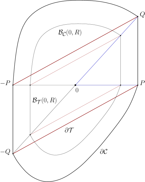
Figure 3. Comparing $\mathcal{B}_{\mathcal{C}{}_{\!}}(0,R)\cap P0Q$ and $\mathcal{B}_{\mathcal{T}{}_{\!}}(0,R)\cap P0Q$

Proof (see Figure 3).

• Point 1. The equality case in Point 1 of Proposition 2.2 proves that any point $p\in{}_{\!}P0Q$ satisfies $d_{\mathcal{C}{}_{\!}}(0,p)=d_{\mathcal{T}{}_{\!}}(0,p)$, and hence we get $\mathcal{S}_{\mathcal{C}{}_{\!}}(0,R)\cap P0Q=\mathcal{S}_{\mathcal{T}{}_{\!}}(0,R)\cap P0Q$.

Then, writing $\displaystyle\mathcal{B}_{\mathcal{C}{}_{\!}}(0,R)=\!\!\!\bigcup_{{}_{\!}r\in[0,R)}\!\!\!{}_{\!}\mathcal{S}_{\mathcal{C}{}_{\!}}(0,r)$, we have $\mathcal{B}_{\mathcal{C}{}_{\!}}(0,R)\cap P0Q=\mathcal{B}_{\mathcal{T}{}_{\!}}(0,R)\cap P0Q$.

• Point 2. The previous point implies

$$\mathcal{B}_{\mathcal{C}{}_{\!}}(0,R)\cap P0Q\ \subseteq\ \mathcal{B}_{\mathcal{T}{}_{\!}}(0,R)\ \subseteq\ \mathcal{T}\ \subseteq\ \mathcal{C}~{},$$

and hence

(2.1) $$\mu_{\mathcal{C}{}_{\!}}\big{(}\mathcal{B}_{\mathcal{C}{}_{\!}}(0,R)\cap P0Q\big{)}\ \leqslant\ \mu_{\mathcal{T}{}_{\!}}(\mathcal{B}_{\mathcal{T}{}_{\!}}(0,R))~{}.$$

Now, if $f$ denotes the unique linear transformation of $\mathbf{R}^{\!2\!}$ such that $f(P)=(1,-1)$ and $f(Q)=(1,1)$, we have

$$f(\mathcal{T})\ =\ \mathcal{Q}\ \mbox{\raisebox{0.366pt}{$:$}\!$=$}\ (-1,1)\!\times\!(-1,1)\subseteq\mathbf{R}^{\!2\!}\quad\mbox{(standard open square)}~{}.$$

The cross ratio being preserved by the linear group $\mathrm{G{}_{\!}L}(\mathbf{R}^{\!2\,\!})$, the map $f$ induces an isometry between the metric spaces $(\mathcal{T},d_{\mathcal{T}{}_{\!}})$ and $(\mathcal{Q},d_{{}_{\!}\mathcal{Q}{}_{\!}})$ with $f(0)=0$, and thus we obtain $\mu_{\mathcal{T}{}_{\!}}(\mathcal{B}_{\mathcal{T}{}_{\!}}(0,R))=\mu_{{}_{\!}\mathcal{Q}{}_{\!}}(\mathcal{B}_{{}_{\!}\mathcal{Q}{}_{\!}}(0,R))$.

But Proposition 2.3 yields

$$\mu_{{}_{\!}\mathcal{Q}{}_{\!}}(\mathcal{B}_{{}_{\!}\mathcal{Q}{}_{\!}}(0,R)) = 8\!\!\int_{\!0}^{\tanh{\!({}_{\!}R)}\,}{\!\!\!\!\left(\int_{\!0}^{x}{\!\!\!\!\frac{\pi}{\mathrm{vol}(B_{{}_{\!}\mathcal{Q}{}_{\!}}(x,y))}\mathrm{d}y}\!\!\right)\!\!\mathrm{d}x}$$

$$\leqslant 4\!\!\int_{\!0}^{\tanh{\!({}_{\!}R)}\,}{\!\!\!\!\left(\int_{\!0}^{x}{\!\!\!\!\frac{\pi}{(1-x^{2}){}_{\!}(1-y^{2})}\mathrm{d}y}\!\!\right)\!\!\mathrm{d}x}\ =\ 2\pi R^{2},$$

which gives $\mu_{\mathcal{C}{}_{\!}}\big{(}\mathcal{B}_{\mathcal{C}{}_{\!}}(0,R)\cap P0Q\big{)}\leqslant 2\pi R^{2}$ from Equation 2.1. ∎

Lemma 2.2.

Let $(\mathcal{C},d_{\mathcal{C}{}_{\!}})$ be a Hilbert domain in $\mathbf{R}^{\!2\!}$ which satisfies $0\in\mathcal{C}\subseteq\mathbf{B}^{{}_{\!}2\!}$, and let $A$, $B$ be two distinct points in $\mathbf{S}^{{}_{\!}1\!}$.

Then for any $R>0$ we have

$$\mu_{\mathcal{C}{}_{\!}}\big{(}\mathcal{B}_{\mathcal{C}{}_{\!}}(0,R)\cap\sphericalangle(A0B)\big{)}\ \leqslant\ \frac{\pi e^{8R}}{\mathrm{vol}(\mathcal{B}_{\mathcal{C}{}_{\!}}(0,1))}\!\times\!\widehat{A0B}{}_{\!}/2~{},$$

where $\widehat{A0B}$ is the spherical distance between the vectors $\overrightarrow{0A}$ and $\overrightarrow{0B}$ (i. e. , the unique number $\theta$ in $[0,\pi]$ defined by $\cos{\theta}=\left\langle\overrightarrow{0A}/\!\left\|\overrightarrow{0A}\right\|\,,\,\overrightarrow{0B}{}_{\!}/\!\left\|\overrightarrow{0B}\right\|\right\rangle\!\in\![-1,1]$, where $\left\langle\cdot\,,\cdot\right\rangle$ stands for the canonical Euclidean scalar product on $\mathbf{R}^{\!2\!}$).

Proof.

Since we have $1/\mathrm{vol}(B_{{}_{\!}\mathcal{C}{}_{\!}}(p))\leqslant e^{8R\!}/\mathrm{vol}(\mathcal{B}_{\mathcal{C}{}_{\!}}(0,R))$ for every $p\in\mathcal{B}_{\mathcal{C}{}_{\!}}(0,R)$ by Proposition 2.4, one can write

$$\mu_{\mathcal{C}{}_{\!}}\big{(}\mathcal{B}_{\mathcal{C}{}_{\!}}(0,R)\cap\sphericalangle(A0B)\big{)} \leqslant \frac{\pi e^{8R}}{\mathrm{vol}(\mathcal{B}_{\mathcal{C}{}_{\!}}(0,R))}\mathrm{vol}\big{(}\mathcal{B}_{\mathcal{C}{}_{\!}}(0,R)\cap\sphericalangle(A0B)\big{)}$$

$$\leqslant \frac{\pi e^{8R}}{\mathrm{vol}(\mathcal{B}_{\mathcal{C}{}_{\!}}(0,1))}\mathrm{vol}\big{(}\mathbf{B}^{{}_{\!}2\!}\cap\sphericalangle(A0B)\big{)}$$

$$(\mbox{noticing $\,\mathcal{B}_{\mathcal{C}{}_{\!}}(0,1)\subseteq\mathcal{B}_{\mathcal{C}{}_{\!}}(0,R)\subseteq\mathbf{B}^{{}_{\!}2\,\!}$})$$

$$= \frac{\pi e^{8R}}{\mathrm{vol}(\mathcal{B}_{\mathcal{C}{}_{\!}}(0,1))}\!\times\!\pi\!\times\!\widehat{A0B}{}_{\!}/{}_{\!}(2\pi)\ =\ \frac{\pi e^{8R}}{\mathrm{vol}(\mathcal{B}_{\mathcal{C}{}_{\!}}(0,1))}\!\times\!\widehat{A0B}{}_{\!}/2~{},$$

where we used $\mathrm{vol}(\mathbf{B}^{{}_{\!}2\,\!})=\pi$. ∎

3. Entropy may not be a limit

We prove in this section the main result of this paper which states that the volume growth entropy for a Hilbert domain may not be a limit. To this end, we will approximate a disc in the plane by an inscribed ‘polygonal’ domain with infinitely many vertices that have two accumulation points around which the boundary of the ‘polygonal’ domain looks very strongly like the boundary of the disc.

Let $\left(n_{k}\right)_{\!k\geqslant 0}$ be the sequence of positive integers defined by

$$n_{0}\ \mbox{\raisebox{0.366pt}{$:$}\!$=$}\ 3\qquad\mbox{and}\qquad\forall\,k\ \geqslant\ 0,\quad n_{k+1}\ =\ 3^{n_{k}^{2}}~{}.$$

It is increasing and satisfies $n_{k}\longrightarrow+\infty$ as $k\longrightarrow+\infty$.

Next, define the sequences $\left(\alpha_{k}\right)_{\!k\geqslant 0}$ and $\left(\theta_{k}\right)_{\!k\geqslant 0}$ in $\mathbf{R}$ by $\alpha_{k}\ \mbox{\raisebox{0.366pt}{$:$}\!$=$}\ 2\pi/n_{k}$ together with

$$\theta_{0}\ \mbox{\raisebox{0.366pt}{$:$}\!$=$}\ 0\qquad\mbox{and}\qquad\forall\,k\geqslant 1,\quad\theta_{k}\ \mbox{\raisebox{0.366pt}{$:$}\!$=$}\ \!\!\sum_{\ell=0}^{k-1}\alpha_{\ell}\ =\ 2\pi\!\sum_{\ell=0}^{k-1}\frac{1}{n_{\ell}}~{}.$$

Finally, consider the sequence $\left(M_{k}\right)_{\!k\geqslant 0}$ and the family $(P_{k\!}(j))_{\!(k,j)\in\{(k,j)\in\mathbf{Z}^{{}^{\!2}}~{}|~{}k\,\geqslant\,0\ \mbox{\tiny and}\ 0\,\leqslant\,j\,\leqslant\,n_{k}\}}$ of points in $\mathbf{S}^{{}_{\!}1\!}$ defined by

$$M_{k}\ \mbox{\raisebox{0.366pt}{$:$}\!$=$}\ (\cos{\!(\theta_{k})}\,,\,\sin{\!(\theta_{k})})\qquad\mbox{and}\qquad P_{k\!}(j)\ \mbox{\raisebox{0.366pt}{$:$}\!$=$}\ (\cos{\!(\theta_{k}+\alpha_{k}j{}_{\!}/{}_{\!}n_{k})}\ ,\ \sin{\!(\theta_{k}+\alpha_{k}j{}_{\!}/{}_{\!}n_{k})})~{},$$

and denote by $\mathcal{C}$ the open convex hull in $\mathbf{R}^{\!2\!}$ of the set

$$\{P_{k\!}(j),-P_{k\!}(j)~{}|~{}k\geqslant 0\,\ \mbox{and}\ \,0\leqslant j\leqslant n_{k}\}~{}.$$

Then we get the following (see Figure 4):

Theorem 3.1.

We have

1. $\displaystyle h(\mathcal{C})\ \mbox{\raisebox{0.366pt}{$:$}\!$=$}\ \!\limsup_{R\rightarrow+\infty}\frac{1}{R}\ln{\![\mu_{\mathcal{C}{}_{\!}}(\mathcal{B}_{\mathcal{C}{}_{\!}}(0,R))]}=1$, and

   
   

2. $\displaystyle\liminf_{R\rightarrow+\infty}\frac{1}{R}\ln{\![\mu_{\mathcal{C}{}_{\!}}(\mathcal{B}_{\mathcal{C}{}_{\!}}(0,R))]}=0$.

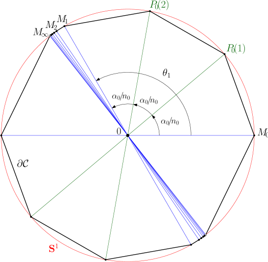
Figure 4. A Hilbert domain in the plane whose entropy is not a limit

Remarks.

1. For all $k\geqslant 0$, one has $P_{k\!}(0)=M_{k}$ and $P_{k\!}(n_{k})=M_{k+1}$.

2. For all $\ell\geqslant 0$, we have $n_{\ell}\geqslant 3^{\ell+1}$ (by induction and using $9^{m}\geqslant m$ for all integer $m\geqslant 0$), and hence the increasing sequence $\left(\theta_{k}\right)_{\!k\geqslant 0}$ converges to some real number $\theta_{\infty}$ which satisfies $0<\theta_{\infty}<\pi$ (since we have $\displaystyle\sum_{\ell=0}^{+\infty}1{}_{\!}/{}_{\!}3^{\ell+1}\,=\,(1{}_{\!}/{}_{\!}3)\!\!\sum_{\ell=0}^{+\infty}(1{}_{\!}/{}_{\!}3)^{\ell}\,=\,1{}_{\!}/{}_{\!}2\,$ and $\,\left(n_{\ell}\right)_{\!\ell\geqslant 0}\,\neq\,\left(3^{\ell+1}\right)_{\!\ell\geqslant 0}$).

In order to prove this theorem, we shall use two different sequences of balls about the origin. The first one corresponds to the sequence of radii $r_{k}\ \mbox{\raisebox{0.366pt}{$:$}\!$=$}\ {}_{\!}\ln{\!(n_{k})}$ for $k\geqslant 0$ that makes look the balls like those in the Klein model $(\mathbf{B}^{{}_{\!}2\!},d_{\mathbf{B}^{{}_{\!}2\!}})$ as $k\longrightarrow+\infty$, from which we get Point 1. The second one corresponds to the sequence of radii $R_{i}\ \mbox{\raisebox{0.366pt}{$:$}\!$=$}\ n_{i}$ for $i\geqslant 0$ that makes look the balls like those in a polygonal domain as $i\longrightarrow+\infty$, leading to Point 2.

Proof of Theorem 3.1.

• Point 1. Since we already have $h(\mathcal{C})\leqslant 1$ by [1, Theorem 3.3], let us prove $h(\mathcal{C})\geqslant 1$.

Consider the sequence of positive numbers $\left(r_{k}\right)_{\!k\geqslant 0}$ defined by $r_{k}\ \mbox{\raisebox{0.366pt}{$:$}\!$=$}\ {}_{\!}\ln{\!(n_{k})}$.

Fix $k\geqslant 0$, and let $(p_{k\!}(j))_{0\,\leqslant\,j\,\leqslant\,n_{k}-1}$ be the sequence of points in $\mathbf{R}^{\!2\!}$ defined by

$$p_{k\!}(j)\,\in\,[0,P_{k\!}(j)]\qquad\mbox{and}\qquad d_{\mathcal{C}{}_{\!}}(0,p_{k\!}(j))\;=\ r_{k}~{}.$$

Then fix $j\in\{0,\ldots,n_{k}-1\}$, and let $P\ \mbox{\raisebox{0.366pt}{$:$}\!$=$}\ P_{k\!}(j)$, $Q\ \mbox{\raisebox{0.366pt}{$:$}\!$=$}\ P_{k\!}(j+1)$, $p\ \mbox{\raisebox{0.366pt}{$:$}\!$=$}\ p_{k\!}(j)$ and $q\ \mbox{\raisebox{0.366pt}{$:$}\!$=$}\ q_{k\!}(j+1)$ (see Figure 5).

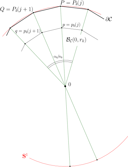
Figure 5. Showing $\displaystyle\limsup_{k\rightarrow+\infty}\frac{\ln{\![\mu_{\mathcal{C}{}_{\!}}(\mathcal{B}_{\mathcal{C}{}_{\!}}(0,r_{k}))]}}{r_{k}}>0$ with $r_{k{}_{\!}}:=\ln{\!(n_{k})}$

First of all, since we have $\mathcal{C}\subseteq\mathbf{B}^{{}_{\!}2\!}$, the equality case in Point 1 of Proposition 2.2 gives

$$r_{k}\ =\ d_{\mathcal{C}{}_{\!}}(0,p)\ =\ d_{\mathbf{B}^{{}_{\!}2\!}}(0,p)\qquad\mbox{and}\qquad r_{k}\ =\ d_{\mathcal{C}{}_{\!}}(0,q)\ =\ d_{\mathbf{B}^{{}_{\!}2\!}}(0,q)~{},$$

which implies

$$\left\|p\right\|\ =\ \left\|q\right\|\ =\ \tanh{\!(r_{k})}$$

by Point 1 of Proposition 2.1.

Therefore, if $a$ denotes the midle point of $p$ and $q$, we get

$$\left\|a\right\|\ =\ \tanh{\!(r_{k})}\cos{\![\alpha_{k}/{}_{\!}(2n_{k})]}\ =\ \tanh{\!(r_{k})}\cos{\!(\pi{}_{\!}/{}_{\!}n_{k}^{2})}~{}.$$

Defining $\rho_{k}\ \mbox{\raisebox{0.366pt}{$:$}\!$=$}\ d_{\mathbf{B}^{{}_{\!}2\!}}(0,a)$ and using again Point 1 of Proposition 2.2 together with the formula $\displaystyle\tanh{\!(\ln{x})}=\frac{x^{2}-1}{x^{2}+1}$ which holds for any $x>0$, one can write

(3.1) $$\begin{split}1-\tanh{\!(\rho_{k})}\ =\ 1-\tanh{\!(r_{k})}\cos{\!(\pi{}_{\!}/{}_{\!}n_{k}^{2})}&\ =\ 1-\frac{n_{k}^{2}-1}{n_{k}^{2}+1}\cos{\!(\pi{}_{\!}/{}_{\!}n_{k}^{2})}\\ &\ =\ 2{}_{\!}/{}_{\!}n_{k}^{2}+\circ{}_{\!}(1{}_{\!}/{}_{\!}n_{k}^{2})\ \sim\ 2{}_{\!}/{}_{\!}n_{k}^{2}\quad\mbox{as}\quad k\longrightarrow+\infty~{}.\end{split}$$

On the other hand, the inclusions

$$\mathcal{B}_{\mathbf{B}^{{}_{\!}2\!}}(0,\rho_{k})\cap P0Q\ \subseteq\ p0q\ \subseteq\ \mathcal{C}\ \subseteq\ \mathbf{B}^{{}_{\!}2\!}$$

yield

$$\mu_{\mathcal{C}{}_{\!}}(p0q)\ \geqslant\ \mu_{\mathbf{B}^{{}_{\!}2\!}}(p0q)\ \geqslant\ \mu_{\mathbf{B}^{{}_{\!}2\!}}(\mathcal{B}_{\mathbf{B}^{{}_{\!}2\!}}(0,\rho_{k})\cap P0Q)\ =\ \frac{\alpha_{k}/{}_{\!}n_{k}}{2\pi}\!\times\!\mu_{\mathbf{B}^{{}_{\!}2\!}}(\mathcal{B}_{\mathbf{B}^{{}_{\!}2\!}}(0,\rho_{k}))$$

by Point 3 of Proposition 2.2 and since Euclidean rotations induce isometries of $(\mathbf{B}^{{}_{\!}2\!},d_{\mathbf{B}^{{}_{\!}2\!}})$, from which one obtains

(3.2) $$\mu_{\mathcal{C}{}_{\!}}(p0q)\ \geqslant\ \frac{\pi}{2}\sinh^{{}_{\!}2{}_{\!}}{\!({}_{\!}\rho_{k})}{}_{\!}/{}_{\!}n_{k}^{2}$$

by Point 2 in Proposition 2.1.

Now, since we have $\sinh^{{}_{\!}2{}_{\!}}{\!(x)}=\tanh^{{}_{\!}2{}_{\!}}{\!(x)}{}_{\!}/{}_{\!}(1-\tanh^{{}_{\!}2{}_{\!}}{\!(x)})$ for all $x\in\mathbf{R}$, Equation 3.1 implies

$$\frac{\pi}{2}\sinh^{{}_{\!}2{}_{\!}}{\!({}_{\!}\rho_{k})}{}_{\!}/{}_{\!}n_{k}^{2}\ \sim\ \pi{}_{\!}/8\quad\mbox{as}\quad k\longrightarrow+\infty~{},$$

from which Equation 3.2 insures the existence of an integer $k_{0}\geqslant 0$ such that

$$\mu_{\mathcal{C}{}_{\!}}(p_{k\!}(j)0p_{k\!}(j+1))\ =\ \mu_{\mathcal{C}{}_{\!}}(p0q)\ \geqslant\ 1{}_{\!}/{}_{\!}3$$

holds for every $k\geqslant k_{0}$.

We then get

$$\mu_{\mathcal{C}{}_{\!}}(\mathcal{B}_{\mathcal{C}{}_{\!}}(0,r_{k}))\ \geqslant\sum_{j=0}^{n_{k}-1}\mu_{\mathcal{C}{}_{\!}}(p_{k\!}(j)0p_{k\!}(j+1))\ \geqslant\ (1{}_{\!}/{}_{\!}3)n_{k}$$

for each $k\geqslant k_{0}$ since we have $p_{k\!}(j)0p_{k\!}(j+1)\subseteq\mathcal{B}_{\mathcal{C}{}_{\!}}(0,r_{k})$ for every $j\in\{0,\ldots,n_{k}-1\}$ (indeed, balls of a Hilbert domain are convex), and hence

$$\frac{\ln{\![\mu_{\mathcal{C}{}_{\!}}(\mathcal{B}_{\mathcal{C}{}_{\!}}(0,r_{k}))]}}{r_{k}}\ \geqslant\ \frac{\ln{\![(1{}_{\!}/{}_{\!}3)n_{k}]}}{\ln{\!(n_{k})}}~{},$$

which yields $\displaystyle\frac{\ln{\![\mu_{\mathcal{C}{}_{\!}}(\mathcal{B}_{\mathcal{C}{}_{\!}}(0,r_{k}))]}}{r_{k}}\longrightarrow 1$ as $k\longrightarrow+\infty$.

This gives the first point of Theorem 3.1.

• Point 2. Consider the sequence of positive numbers $\left(R_{i}\right)_{\!i\geqslant 0}$ defined by $R_{i}\ \mbox{\raisebox{0.366pt}{$:$}\!$=$}\ n_{i}$.

Fixing an integer $i\geqslant 0$, we can write the decomposition

(3.3) $$\begin{split}\frac{1}{2}\mu_{\mathcal{C}{}_{\!}}(\mathcal{B}_{\mathcal{C}{}_{\!}}(0,R_{i}))&\ =\ \mu_{\mathcal{C}{}_{\!}}\big{(}\mathcal{B}_{\mathcal{C}{}_{\!}}(0,R_{i})\cap-M_{\infty}0M_{0}\big{)}\\ &\ +\,\sum_{k=0}^{i}\sum_{j=0}^{n_{k}-1}\mu_{\mathcal{C}{}_{\!}}\big{(}\mathcal{B}_{\mathcal{C}{}_{\!}}(0,R_{i})\cap P_{k\!}(j)0P_{k\!}(j+1)\big{)}\\ &\ +\ \mu_{\mathcal{C}{}_{\!}}\big{(}\mathcal{B}_{\mathcal{C}{}_{\!}}(0,R_{i})\cap\sphericalangle(M_{i+1}0M_{\infty})\big{)}\end{split}$$

with $M_{\infty}\ \mbox{\raisebox{0.366pt}{$:$}\!$=$}\ (\cos{\!(\theta_{\infty})}\,,\,\sin{\!(\theta_{\infty})})\in\partial\mathcal{C}$ (recall that $\theta_{\infty}$ is the limit of the sequence $\left(\theta_{k}\right)_{\!k\in\mathbf{N}}$: see the second remark following Theorem 3.1).

* First step. Here, we deal with the two first terms in Equation 3.3.

For each $k\geqslant 0$ and $j\in\{0,\ldots,n_{k}-1\}$, let $\mathcal{T}_{k}(j)$ be the open rectangle that is equal to the open convex hull in $\mathbf{R}^{\!2\!}$ of $P_{k\!}(j)$, $-P_{k\!}(j)$, $P_{k\!}(j+1)$ and $-P_{k\!}(j+1)$.

Then, by Lemma 2.1, we have

(3.4) $$\mu_{\mathcal{C}{}_{\!}}\big{(}\mathcal{B}_{\mathcal{C}{}_{\!}}(0,R_{i})\cap P_{k\!}(j)0P_{k\!}(j+1)\big{)}\ \leqslant\ 2\pi R_{i}^{2}$$

and

(3.5) $$\mu_{\mathcal{C}{}_{\!}}\big{(}\mathcal{B}_{\mathcal{C}{}_{\!}}(0,R_{i})\cap-M_{\infty}0M_{0}\big{)}\ \leqslant\ 2\pi R_{i}^{2\!}~{}.$$

* Second step. Next, we focus on the third term in Equation 3.3.

Lemma 2.2 with $\displaystyle\widehat{M_{i+1}0M_{\infty}}=\theta_{\infty}-\theta_{i+1}=\,2\pi\!\!\!\sum_{\ell=i+1}^{+\infty}\!\!1{}_{\!}/{}_{\!}n_{\ell}$ implies

(3.6) $$\mu_{\mathcal{C}{}_{\!}}\big{(}\mathcal{B}_{\mathcal{C}{}_{\!}}(0,R_{i})\cap\sphericalangle(M_{i+1}0M_{\infty})\big{)}\ \leqslant\ \tau\!\sum_{\ell=i}^{+\infty}e^{8R_{i}\!}{}_{\!}/{}_{\!}n_{\ell+1}~{},$$

where $\tau\ \mbox{\raisebox{0.366pt}{$:$}\!$=$}\ \pi^{2}\!{}_{\!}/{}_{\!}\mathrm{vol}(\mathcal{B}_{\mathcal{C}{}_{\!}}(0,1))$ is a positive constant.

But for any $\ell\geqslant i$ we have

$$e^{8R_{i}\!}{}_{\!}/{}_{\!}n_{\ell+1}\ =\ e^{8R_{i}}3^{-n_{\ell}^{2}}\ \leqslant\ 3^{8R_{i}}3^{-n_{\ell}^{2}}\ =\ 3^{8n_{i}-n_{\ell}^{2}}\ =\ 3^{-n_{\ell}^{2}(1-8n_{i}/{}_{\!}n_{\ell}^{2})}$$

with $n_{i}/{}_{\!}n_{\ell}^{2}\leqslant 1{}_{\!}/{}_{\!}n_{i}$ from the monotone increasing of the sequence $\left(n_{\ell}\right)_{\!\ell\geqslant 0}$.

Hence, since $1{}_{\!}/{}_{\!}n_{i}\longrightarrow 0$ as $i\longrightarrow+\infty$, there exists an integer $i_{0}\geqslant 0$ such that for all $\ell\geqslant i$ one has $e^{8R_{i}\!}{}_{\!}/{}_{\!}n_{\ell+1}\leqslant 3^{-n_{\ell}^{2{}_{\!}}/2}$ whenever $i\geqslant i_{0}$.

Equation 3.6 then implies

$$\mu_{\mathcal{C}{}_{\!}}\big{(}\mathcal{B}_{\mathcal{C}{}_{\!}}(0,R_{i})\cap\sphericalangle(M_{i+1}0M_{\infty})\big{)}\ \leqslant\ \tau\!\sum_{\ell=i}^{+\infty}3^{-n_{\ell}^{2{}_{\!}}/2}\ \leqslant\ \tau\!\sum_{\ell=i}^{+\infty}3^{-\ell}\ =\ 3^{-i+1}\tau{}_{\!}/2$$

for all $i\geqslant i_{0}$ (notice that we have $n_{\ell}^{2{}_{\!}}/2\geqslant 9^{\ell}\geqslant\ell$ for any $\ell\geqslant 0$: see the second remark following Theorem 3.1).

Now we have $3^{-i}\longrightarrow 0$ as $i\longrightarrow+\infty$, and thus there exists an integer $i_{1}\geqslant i_{0}$ such that for all $i\geqslant i_{1}$ one has

(3.7) $$\mu_{\mathcal{C}{}_{\!}}\big{(}\mathcal{B}_{\mathcal{C}{}_{\!}}(0,R_{i})\cap\sphericalangle(M_{i+1}0M_{\infty})\big{)}\ \leqslant\ 1~{}.$$

* Third step. Combining Equations 3.3, 3.4, 3.5 and 3.7, we eventually get

$$\begin{split}\mu_{\mathcal{C}{}_{\!}}(\mathcal{B}_{\mathcal{C}{}_{\!}}(0,R_{i}))&\ \leqslant\ 4\pi R_{i}^{2}{}_{\!}+4\pi R_{i}^{2}\!\sum_{k=0}^{i}n_{k}+1\\ &\ \leqslant\ 4\pi R_{i}^{2}{}_{\!}+4\pi R_{i}^{2}(i+1)n_{i}+1\\ &\qquad(\mbox{since the sequence $\left(n_{k}\right)_{\!k\geqslant 0}$ is non-decreasing})\\ &\ =\ 4\pi R_{i}^{2}{}_{\!}+4\pi(i+1)R_{i}^{3}{}_{\!}+1\\ &\ \leqslant\ 12\pi R_{i}^{4}\end{split}$$

for all $i\geqslant i_{1}$ (since we have $R_{\ell}\ \mbox{\raisebox{0.366pt}{$:$}\!$=$}\ n_{\ell}\geqslant 3^{\ell+1}\geqslant\ell+1\geqslant 1$ for every $\ell\geqslant 0$), and hence

$$\frac{\ln{\![\mu_{\mathcal{C}{}_{\!}}(\mathcal{B}_{\mathcal{C}{}_{\!}}(0,1))]}}{R_{i}}\ \leqslant\ \frac{\ln{\![\mu_{\mathcal{C}{}_{\!}}(\mathcal{B}_{\mathcal{C}{}_{\!}}(0,R_{i}))]}}{R_{i}}\ \leqslant\ \frac{\ln{\!(12\pi R_{i}^{4})}}{R_{i}}~{},$$

which yields $\displaystyle\frac{\ln{\![\mu_{\mathcal{C}{}_{\!}}(\mathcal{B}_{\mathcal{C}{}_{\!}}(0,R_{i}))]}}{R_{i}}\longrightarrow 0$ as $i\longrightarrow+\infty$.

This proves the second point of Theorem 3.1. ∎

Remark.

Considering the proof of Point 1 in Theorem 3.1, we can observe that the conclusion $h(\mathcal{C})>0$ we obtained is actually true for any sequence of positive integers $\left(n_{k}\right)_{\!k\geqslant 0}$ provided the sequence $\left(\theta_{k}\right)_{\!k\in\mathbf{N}}$ converges to some real number $\theta_{\infty}$ which satisfies $0<\theta_{\infty}<\pi$.

4. Non-polygonal domains may have zero entropy

In this section, we construct a Hilbert domain in the plane which is a ‘polygon’ having infinitely many vertices and whose volume growth entropy is a limit that is equal to zero. This ‘polygon’ is inscribed in a circle and its vertices have one accumulation point.

Before giving our example, let us first recall the following result proved in [15]:

Theorem 4.1.

Given any open convex polytope $\mathcal{P}$ in $\mathbf{R}^{\!m\!}$ that contains the origin $0$, the volume growth entropy of $d_{\mathcal{P}{}_{\!}}$ satisfies

$$h(\mathcal{P})\ =\lim_{R\rightarrow+\infty}\frac{1}{R}\ln{\![\mu_{\mathcal{P}{}_{\!}}(\mathcal{B}_{\mathcal{P}{}_{\!}}(0,R))]}\ =\ 0~{}.$$

Remark.

Another — but less direct — proof of this theorem consists in saying that $(\mathcal{P},d_{\mathcal{P}{}_{\!}})$ is Lipschitz equivalent to Euclidean plane as shown in [2] (and in [8] for the particular case when $n\ \mbox{\raisebox{0.366pt}{$:$}\!$=$}\ 2$), and hence $h(\mathcal{P})=0$ since the volume growth entropy of any finite-dimensional normed vector space is equal to zero.

Now, let us show that having zero volume growth entropy for a Hilbert domain in $\mathbf{R}^{\!2\!}$ does not mean being polygonal, that is, that the converse of Theorem 4.1 is false.

Let $\left(P_{n}\right)_{\!n\in\mathbf{N}}$ be the sequence of points in $\mathbf{S}^{{}_{\!}1\!}$ defined by

$$P_{n}\ \mbox{\raisebox{0.366pt}{$:$}\!$=$}\ (\cos{\!(2^{-n})}\,,\,\sin{\!(2^{-n})})~{},$$

and denote by $\mathcal{C}$ the open convex hull in $\mathbf{R}^{\!2\!}$ of the set

$$\{P_{n},-P_{n}~{}|~{}n\in\mathbf{N}\}~{}.$$

Then we have (see Figure 6)

Theorem 4.2.

The volume growth entropy of $d_{\mathcal{C}{}_{\!}}$ satisfies

$$h(\mathcal{C})\ =\lim_{R\rightarrow+\infty}\frac{1}{R}\ln{\![\mu_{\mathcal{C}{}_{\!}}(\mathcal{B}_{\mathcal{C}{}_{\!}}(0,R))]}\ =\ 0~{}.$$

Remark.

More precisely, we will show in the proof of this result that the volume $\mu_{\mathcal{C}{}_{\!}}(\mathcal{B}_{\mathcal{C}{}_{\!}}(0,R))$ of the ball $\mathcal{B}_{\mathcal{C}{}_{\!}}(0,R)$ actually has at most the same growth as $R^{3}$ when $R$ goes to infinity.

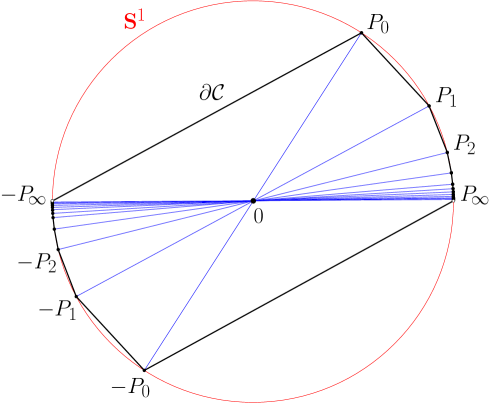
Figure 6. A non-polygonal Hilbert domain in the plane with zero entropy

Proof of Theorem 4.2.

Fixing an integer $n\geqslant 0$ and a number $R\geqslant 1$, we can use again the decomposition given by Equation 3.3 in the proof of the second point of Theorem 3.1 and write

(4.1) $$\begin{split}\frac{1}{2}\mu_{\mathcal{C}{}_{\!}}(\mathcal{B}_{\mathcal{C}{}_{\!}}(0,R))&\ =\ \mu_{\mathcal{C}{}_{\!}}\big{(}\mathcal{B}_{\mathcal{C}{}_{\!}}(0,R)\cap-P_{\!\infty}0P_{0}\big{)}\\ &\ +\,\sum_{k=0}^{n}\mu_{\mathcal{C}{}_{\!}}\big{(}\mathcal{B}_{\mathcal{C}{}_{\!}}(0,R)\cap P_{k}0P_{k+1}\big{)}\\ &\ +\ \mu_{\mathcal{C}{}_{\!}}\big{(}\mathcal{B}_{\mathcal{C}{}_{\!}}(0,R)\cap\sphericalangle(P_{n+1}0P_{\!\infty})\big{)}\end{split}$$

with $\displaystyle P_{\!\infty}\ \mbox{\raisebox{0.366pt}{$:$}\!$=$}\ (1,0)=\!\!\!\lim_{k\rightarrow+\infty}\!\!\!P_{k}\in\partial\mathcal{C}$.

• First step. Here, we deal with the two first terms in Equation 4.1.

For each $k\in\mathbf{N}$, let $\mathcal{T}_{k}$ be the open rectangle that is equal to the open convex hull in $\mathbf{R}^{\!2\!}$ of $P_{k}$, $-P_{k}$, $P_{k+1}$ and $-P_{k+1}$.

Then, by Lemma 2.1, we have

(4.2) $$\mu_{\mathcal{C}{}_{\!}}\big{(}\mathcal{B}_{\mathcal{C}{}_{\!}}(0,R)\cap P_{k}0P_{k+1}\big{)}\ \leqslant\ 2\pi R^{2}$$

and

(4.3) $$\mu_{\mathcal{C}{}_{\!}}\big{(}\mathcal{B}_{\mathcal{C}{}_{\!}}(0,R)\cap-P_{\!\infty}0P_{0}\big{)}\ \leqslant\ 2\pi R^{2}.$$

• Second step. Next, we focus on the third term in Equation 4.1.

As in the second step of the proof of the second point of Theorem 3.1, we use again Lemma 2.2 with $\widehat{P_{n+1}0P_{\!\infty}}=2^{-(n+1)}-0=2^{-(n+1)}$ to get

(4.4) $$\mu_{\mathcal{C}{}_{\!}}\big{(}\mathcal{B}_{\mathcal{C}{}_{\!}}(0,R)\cap\sphericalangle(P_{n+1}0P_{\!\infty})\big{)}\ \leqslant\ \tau e^{8R}\!{}_{\!}\times\!2^{-n},$$

where $\tau\ \mbox{\raisebox{0.366pt}{$:$}\!$=$}\ \pi{}_{\!}/{}_{\!}(4\,\mathrm{vol}(\mathcal{B}_{\mathcal{C}{}_{\!}}(0,1)))$ is a positive constant.

So, if we choose $n\ \mbox{\raisebox{0.366pt}{$:$}\!$=$}\ [12R]+1$ (where $[\,\cdot\,]$ denotes the integer part), we have $e^{8R}\!{}_{\!}\times\!2^{-n}\leqslant 1$, and hence Equation 4.4 implies

(4.5) $$\mu_{\mathcal{C}{}_{\!}}\big{(}\mathcal{B}_{\mathcal{C}{}_{\!}}(0,R)\cap\sphericalangle(P_{n+1}0P_{\!\infty})\big{)}\ \leqslant\ \tau~{}.$$

• Third step. Combining Equations 4.1, 4.2, 4.3 and 4.5, we eventually obtain

$$\begin{split}\mu_{\mathcal{C}{}_{\!}}(\mathcal{B}_{\mathcal{C}{}_{\!}}(0,R))&\ \leqslant\ 4\pi R^{2}\!+4\pi(n+1)R^{2}\!+\tau\\ &\ \leqslant\ 4\pi R^{2}\!+4\pi(12R+2)R^{2}\!+\tau\\ &\qquad(\mbox{since one has $\,n-1=[12R]\leqslant 12R$})\\ &\ \leqslant\ (144\pi+\tau)R^{3}\end{split}$$

for any $R\geqslant 1$, and hence

$$\frac{\ln{\![\mu_{\mathcal{C}{}_{\!}}(\mathcal{B}_{\mathcal{C}{}_{\!}}(0,1))]}}{R}\ \leqslant\ \frac{\ln{\![\mu_{\mathcal{C}{}_{\!}}(\mathcal{B}_{\mathcal{C}{}_{\!}}(0,R))]}}{R}\ \leqslant\ \frac{\ln{\!((144\pi+\tau)R^{3})}}{R}~{},$$

which yields $\displaystyle\frac{\ln{\![\mu_{\mathcal{C}{}_{\!}}(\mathcal{B}_{\mathcal{C}{}_{\!}}(0,R))]}}{R}\longrightarrow 0$ as $R\longrightarrow+\infty$.

This proves Theorem 4.2. ∎

References

- [1] Berck, G., Bernig, A., and Vernicos, C. Volume entropy of Hilbert geometries. Pac. J. Math. 245, 2 (2010), 201–225.
- [2] Bernig, A. Hilbert geometry of polytopes. Arch. Math. 92 (2009), 314–324.
- [3] Burago, D., Burago, Y., and Ivanov, S. A course in metric geometry. AMS, 2001.
- [4] Busemann, H. The geometry of geodesics. Academic Press, 1955.
- [5] Busemann, H., and Kelly, P. Projective geometry and projective metrics. Academic Press, 1953.
- [6] Colbois, B., and Vernicos, C. Bas du spectre et delta-hyperbolicité en géométrie de Hilbert plane. Bull. Soc. Math. Fr. 134, 3 (2006), 357–381.
- [7] Colbois, B., Vernicos, C., and Verovic, P. L’aire des triangles idéaux en géométrie de Hilbert. Enseign. Math. 50, 3-4 (2004), 203–237.
- [8] Colbois, B., Vernicos, C., and Verovic, P. Hilbert geometry for convex polygonal domains. J. Geom. 100 (2011), 37–64.
- [9] Colbois, B., and Verovic, P. Hilbert geometry for strictly convex domains. Geom. Dedicata 105 (2004), 29–42.
- [10] Crampon, M. Entropies of compact strictly convex projective manifolds. JMD 3, 4 (2009), 511–547.
- [11] Egloff, D. Uniform Finsler Hadamard manifolds. Ann. Inst. Henri Poincaré, Phys. Théor. 66 (1997), 323–357.
- [12] Goldman, W. Projective geometry on manifolds. Lecture notes, University of Maryland, 1988.
- [13] Socié-Méthou, É. Comportements asymptotiques et rigidités des géométries de Hilbert. PhD thesis, University of Strasbourg, 2000.
- [14] Vernicos, C. Introduction aux géométries de Hilbert. Sémin. Théor. Spectr. Géom. 23 (2005), 145–168.
- [15] Vernicos, C. Spectral radius and amenability in Hilbert geometry. Houston J. Math. 35, 4 (2009), 1143–1169.
- [16] Vinberg, E. Geometry II. Springer, 1993.