Distributed entanglement induced by dissipative bosonic media

Abstract

We describe a scheme with analytic result that allows to generate steady-state entanglement for two atoms over a dissipative bosonic medium. The resonant coupling between the mediating bosonic mode and cavity modes produces three collective atomic decay channels. This dissipative dynamics, together with the unitary process induced by classical microwave fields, drives the two atoms to the symmetric or asymmetric entangled steady state conditional upon the choice of the phases of the microwave fields. The effects on the steady-state entanglement of off-resonance mediating bosonic modes are analyzed. The entanglement can be obtained with high fidelity regardless of the initial state and there is a linear relation in the scaling of the fidelity with the cooperativity parameter. The fidelity is insensitive to the fluctuation of the Rabi frequencies of the classical driving fields.

1 Introduction

Quantum entanglement plays a crucial role in performing quantum information processing [1, 2, 3, 4], and it is the basic requirement for quantum communication to transfer quantum state between distant locations. To construct quantum networks, one needs to generate spatially separate qubits, store them for sufficiently long time, and perform logic operations between them. Therefore, the generation of entanglement between different nodes becomes an important task [5]. The optical absorption and other channel noise inevitably bring the detrimental effects to the entanglement between distant nodes, which normally decreases exponentially with the length of the connecting medium. The quantum communication difficulty cannot be solved just based on unitary dynamics [6, 7, 8, 9, 10, 11, 12, 13, 14].

To overcome the problem associated with the exponential fidelity decay of distributed entanglement, the concept of dissipative dynamics can be used, which utilizes the dissipation as a resource for quantum state engineering [15, 16, 17, 18, 19, 20, 21, 22, 23, 24, 25, 26, 27, 28, 29, 30, 31, 32, 33, 34, 35, 36, 37]. Recently, experimental realization of dissipative state preparation has also been reported [38]. Here, we describe a scheme with analytic result that allows to generate steady-state entanglement for two atoms over a dissipative bosonic medium. Compared with the previous scheme we proposed in Ref. [18], the steady entanglement can be produced over a longer distance via a dissipative mediating mode, and is very useful for testing quantum nonlocality [39], quantum secret sharing [40] and quantum communication [41].

Due to the coherent cavity-medium coupling, the system becomes mathematically equivalent to the case that two distant atoms collectively interact with three nondegenerate delocalized field modes, one mode inducing the asymmetric collective atomic decay channel and the other two inducing the symmetric collective atomic decay channels. The decay channels induced by three delocalized field modes are analytically resolved with the dissipative dynamics. Analytical result indicates that the distributed entanglement can be obtained with high fidelity requiring neither the unitary feedback control nor the photon detection. The steady-state entanglement arises from the competition between the collective atomic decays and the unitary evolution induced by the classical microwave fields, which act as a push button to start the dynamical process. We find that the scaling of fidelity $F$ with the cooperativity parameter $C$ is linear. Besides, the effect on the steady-state entanglement of dispersive mediating modes analyzed. We find that the couplings between the dispersive mediating modes and cavity modes lead to the frequency shifts of the normal delocalized bosonic modes, when one of these modes is resonant with the classical laser field, the Raman transitions between two atomic ground states dominate the atom-field coupling dynamics and destroy the process of the steady-state entanglement preparation. The steady-state entanglement is faithfully prepared when the frequency space of the mediating bosonic modes is large enough, showing that our scheme can work well even when many mediating bosonic modes are involved.

2 The theoretical model

As shown in Fig. 1, two three-level atoms are individually trapped in two single-mode cavities linked by a dissipative bosonic medium (a third cavity or a waveguide). Each coherent driving $\Omega$ pumps the ground state $|0\rangle$ to the excited state $|2\rangle$ with the detuning $\Delta$. Atom-cavity interaction $g$ drives the transition $|1\rangle$ $\leftrightarrow$ $|2\rangle$ with the detuning $\Delta-\delta$, and two ground states are coupled by a resonant microwave $\Omega_{M}$ in each cavity.

We assume two cavity modes are coupled to the mediating mode. Then the Hamiltonian of the whole system in the interaction picture can be written as $H_{I}$ = $H_{0}$ + $H_{g}$ + $V_{+}$ + $V_{-}$:

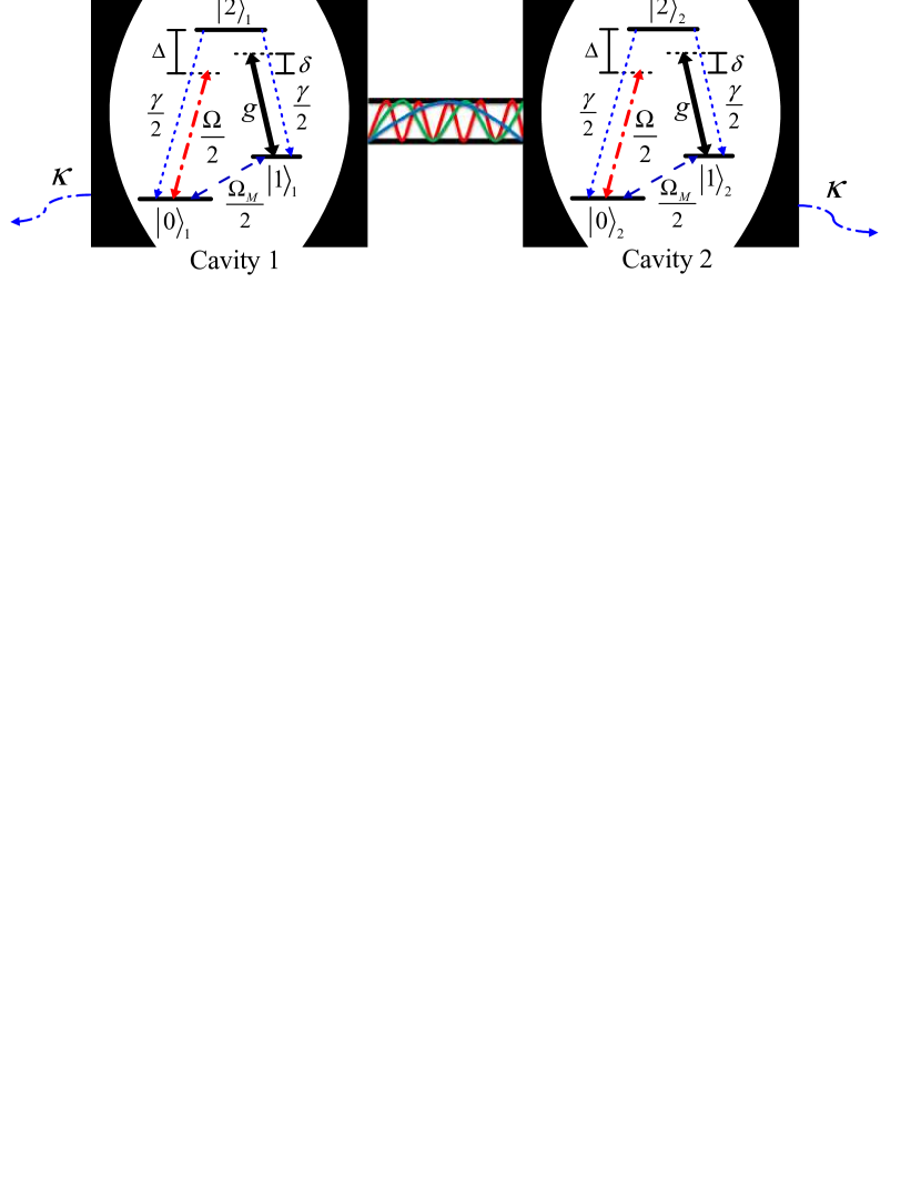
Figure 1: (Color online) Experimental setup and level diagram for dissipative preparation of long-distance entanglement between two atoms coupled to two cavities respectively, which are connected by a multi-mode dissipative medium.

$$H_{0} = \sum_{i=1}^{2}(\Delta|2\rangle_{i}\langle 2|+\delta a_{i}^{{\dagger}}a_{i})+\sum_{i=1}^{2}(g|2\rangle_{i}\langle 1|a_{i}+H.c.)$$ (2)

$$+\sum_{n}^{N}\bigg{\{}(\Delta_{n}+\delta)b_{n}^{\dagger}b_{n}+[\nu_{n}b_{n}(a_{1}^{{\dagger}}+a_{2}^{{\dagger}})+H.c.]\bigg{\}},$$

$$H_{g} = \frac{\Omega_{M}}{2}(|1\rangle_{1}\langle 0|+e^{-i\theta_{M}}|1\rangle_{2}\langle 0|)+H.c.,$$ (4)

$$V_{+} = \frac{\Omega}{2}(|2\rangle_{1}\langle 0|+|2\rangle_{2}\langle 0|),$$ (5)

$$V_{-} = \frac{\Omega}{2}(|0\rangle_{1}\langle 2|+|0\rangle_{2}\langle 2|),$$ (6)

where $a_{i}$ ($i=1,2$) is the annihilation operator for the $i$th cavity field mode, $b_{n}$ is the annihilation operator for the $n$th mediating mode, $\Delta_{n}$ denotes the frequency difference between the $n$th mediating mode and the cavity mode. $\nu_{n}$ denotes the coupling strength between the $i$th cavity mode and the $n$th mediating mode, $g$ is the atom-cavity coupling constant, $\Omega$ and $\Omega_{M}$ represent the classical laser driving strength and the microwave driving strength, respectively. $\theta_{M}$ is the phase difference between the two microwave fields applied to atoms $1$ and $2$. The cavity-mediating couplings are assumed to be the same for all the mediating modes, i.e., $\nu_{n}$ $=$ $\nu$.

To analyze the main dissipation mechanism easily, we first focus on the case that only one mediating mode (i.e., the first mediating mode $b_{1}$) resonantly interacts with the cavity mode and the other mediating modes with large detuning can be neglected in $H_{0}$. Let us define the symmetric steady-state $|T\rangle$ $=$ $\big{(}|10\rangle+|01\rangle\big{)}/\sqrt{2}$, the asymmetric steady-state $|S\rangle$ $=$ $\big{(}|10\rangle-|01\rangle\big{)}/\sqrt{2}$, and introduce three normal delocalized bosonic modes as $c_{1}$ $=$ $(a_{1}-a_{2})/\sqrt{2}$, $c_{2}$ $=$ $(a_{1}+a_{2}+\sqrt{2}b_{1})/2$, and $c_{3}$ $=$ $(a_{1}+a_{2}-\sqrt{2}b_{1})/2$. In terms of the new operators, the Hamiltonian $H_{0}$ becomes

$$H_{0} = \Delta(|2\rangle_{1}\langle 2|+|2\rangle_{2}\langle 2|)$$ (13)

$$+\bigg{[}g|2\rangle_{1}\langle 1|(\frac{1}{2}c_{2}+\frac{1}{2}c_{3}+\frac{\sqrt{2}}{2}c_{1})$$

$$+g|2\rangle_{2}\langle 1|(\frac{1}{2}c_{2}+\frac{1}{2}c_{3}-\frac{\sqrt{2}}{2}c_{1})+H.c.\bigg{]}$$

$$+\delta c_{1}^{\dagger}c_{1}+(\delta+\sqrt{2}\nu)c_{2}^{\dagger}c_{2}+(\delta-\sqrt{2}\nu)c_{3}^{\dagger}c_{3}.$$

Here, $H_{0}$ describes the asymmetric coupling for two atoms to the delocalized field mode $c_{1}$, and the symmetric couplings to $c_{2}$ and $c_{3}$. Because of the cavity-medium coupling, all the delocalized field modes are nondegenerate and each causes a collective dissipation channel. $\kappa_{i}$ $(i=1,2)$ and $\kappa_{3}$ represent the photon decay rate of cavity $i$ and the medium, respectively. $\gamma_{0}$ and $\gamma_{1}$ denote the atomic spontaneous emission rates for $|2\rangle$ $\rightarrow$ $|0\rangle$ and $|2\rangle$ $\rightarrow$ $|1\rangle$, respectively. For simplicity we here set $\kappa_{1}$ $=$ $\kappa_{2}$ $=$ $\kappa_{3}$ $=$ $\kappa$ and $\gamma_{0}$ = $\gamma_{1}$ $=$ $\gamma/2$. Then the corresponding Lindblad operators associated with the photon decay and atomic spontaneous emission can be expressed as $L^{\kappa_{1}}$ = $\sqrt{\kappa}$ $c_{1}$, $L^{\kappa_{2}}$ = $\sqrt{\kappa}$ $c_{2}$, $L^{\kappa_{3}}$ = $\sqrt{\kappa}$ $c_{3}$, $L^{\gamma_{1}}$ = $\sqrt{\gamma_{0}}$ $|0\rangle_{1}\langle 2|$, $L^{\gamma_{2}}$ = $\sqrt{\gamma_{0}}$ $|0\rangle_{2}\langle 2|$, $L^{\gamma_{3}}$ = $\sqrt{\gamma_{1}}$ $|1\rangle_{1}\langle 2|$, $L^{\gamma_{4}}$ = $\sqrt{\gamma_{1}}$ $|1\rangle_{2}\langle 2|$.

Under the condition that the classical laser fields are weak, we can apply the method based on the second-order perturbation theory to tailor the effective dissipation process [15, 16, 17]. Then the dynamics of our distributed cavity QED system is governed by the effective Hamiltonian $H_{eff}$ and effective Lindblad operator $L_{eff}^{x}$:

$$H_{eff} = -\frac{1}{2}V_{-}[H^{-1}_{NH}+(H^{-1}_{NH})^{{\dagger}}]V_{+}+H_{g},$$ (14)

$$L_{eff}^{x} = L^{x}H^{-1}_{NH}V_{+},$$ (15)

where $H^{-1}_{NH}$ is the inverse of the non-Hermitian Hamiltonian $H_{NH}$ = $H_{0}$ $-$ $\frac{i}{2}\sum_{x}(L^{x})^{{\dagger}}L^{x}$, and its elements determine the strength of effective evolution process. The resulting effective master equation in Lindblad form becomes

$$\dot{\rho} = i[\rho,H_{eff}]+\sum_{x}\{L_{eff}^{x}\rho(L_{eff}^{x})^{{\dagger}}$$ (17)

$$-\frac{1}{2}[(L_{eff}^{x})^{{\dagger}}L_{eff}^{x}\rho+\rho(L_{eff}^{x})^{{\dagger}}L_{eff}^{x}]\},$$

$$H_{eff} = -Re[\Omega^{2}\widetilde{R}_{1}]|00\rangle\langle 00|-Re[\frac{\Omega^{2}}{4}\widetilde{R}_{2}]|S\rangle\langle S|$$ (19)

$$-Re[\frac{\Omega^{2}}{4}\widetilde{R}_{3}]|T\rangle\langle T|+H_{g},$$

$$L_{e}^{\kappa_{1}} = \sqrt{\frac{(\delta^{2}-2\nu^{2})^{2}g_{e}^{2}\kappa/4}{A^{2}+B^{2}}}|S\rangle\langle 00|$$ (21)

$$+\sqrt{\frac{g_{e}^{2}\kappa/8}{C_{1}^{2}+D_{1}^{2}}}|11\rangle\langle S|,$$

$$L_{e}^{\kappa_{2}} = \sqrt{\frac{\delta^{2}(\delta-\sqrt{2}\nu)^{2}g_{e}^{2}\kappa/8}{A^{2}+B^{2}}}|T\rangle\langle 00|$$ (23)

$$+\sqrt{\frac{(\delta-\sqrt{2}\nu)^{2}g_{e}^{2}\kappa/16}{C_{2}^{2}+D_{2}^{2}}}|11\rangle\langle T|,$$

$$L_{e}^{\kappa_{3}} = \sqrt{\frac{\delta^{2}(\delta+\sqrt{2}\nu)^{2}g_{e}^{2}\kappa/8}{A^{2}+B^{2}}}|T\rangle\langle 00|$$ (25)

$$+\sqrt{\frac{(\delta+\sqrt{2}\nu)^{2}g_{e}^{2}\kappa/16}{C_{2}^{2}+D_{2}^{2}}}|11\rangle\langle T|,$$

where $Re[$ $]$ denotes the real part of the argument,

$$g_{e} = g\Omega,\delta^{{}^{\prime}}=\delta-i\kappa/2,\Delta^{{}^{\prime}}=\Delta-i\gamma/2,$$ (26)

$$\widetilde{R}_{1} = \frac{\delta^{{}^{\prime}}(\delta^{{}^{\prime}2}-2\nu^{2})}{\Delta^{{}^{\prime}}\delta^{{}^{\prime}}(\delta^{{}^{\prime}2}-2\nu^{2})-g^{2}(\delta^{{}^{\prime}2}-\nu^{2})},$$ (27)

$$\widetilde{R}_{2} = \frac{\Delta^{{}^{\prime}}\delta^{{}^{\prime}}(\delta^{{}^{\prime}2}-2\nu^{2})-g^{2}\delta^{{}^{\prime}2}}{(g^{2}-\delta^{{}^{\prime}}\Delta^{{}^{\prime}})(\delta^{{}^{\prime}2}\Delta^{{}^{\prime}}-\delta^{{}^{\prime}}g^{2}+2\Delta^{{}^{\prime}}\nu^{2})},$$ (28)

$$\widetilde{R}_{3} = \frac{\Delta^{{}^{\prime}}\delta^{{}^{\prime}}(\delta^{{}^{\prime}2}-2\nu^{2})-g^{2}(\delta^{{}^{\prime}2}-2\nu^{2})}{(g^{2}-\delta^{{}^{\prime}}\Delta^{{}^{\prime}})(\delta^{{}^{\prime}2}\Delta^{{}^{\prime}}-\delta^{{}^{\prime}}g^{2}+2\Delta^{{}^{\prime}}\nu^{2})},$$ (29)

$$A = \Delta\delta(\delta^{2}-2\nu^{2})-g^{2}(\delta^{2}-\nu^{2}),$$ (30)

$$B = (\delta/2-\nu^{2})(\Delta\kappa+\gamma\delta)+\delta\kappa(\Delta\delta-g^{2}),$$ (31)

$$C_{1} = g^{2}-\Delta\delta,$$ (32)

$$D_{1} = (\Delta\kappa+\delta\gamma)/2,$$ (33)

$$C_{2} = g^{2}\delta-\Delta(\delta^{2}-2\nu^{2}),$$ (34)

$$D_{2} = \kappa(\Delta\delta-g^{2}/2)+\gamma(\delta^{2}-2\nu^{2})/2.$$ (35)

Since $\Omega$ is very small, we can neglect those terms containing the effective shifts $\mathcal{O}(\Omega^{2})$ in Eq. (9), so that $H_{eff}$ $\simeq$ $H_{g}$. There are three primarily effective decay channels characterized by $L_{e}^{\kappa_{1}}$, $L_{e}^{\kappa_{2}}$, $L_{e}^{\kappa_{3}}$ through three delocalized bosonic modes $c_{1}$, $c_{2}$, $c_{3}$, respectively. It is the mediating mode that links the two separate field modes and lifts the degeneracy of three delocalized field modes, leading to three independent decay channels. We assume $\kappa$, $\gamma$ $\ll$ $g$, $\delta$, $\nu$, $\Delta$, so that the minor terms with higher order than $\kappa^{2}$, $\gamma^{2}$ and $\kappa\gamma$ in the denominators of $L_{e}^{\kappa_{1}}$, $L_{e}^{\kappa_{2}}$ and $L_{e}^{\kappa_{3}}$ have been omitted.

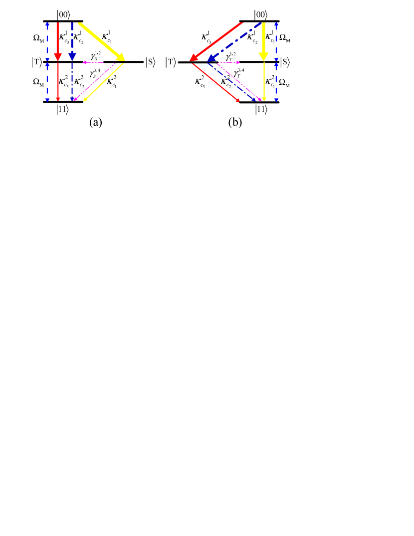
Figure 2: (Color online) Effective two qubit system for coherent and dissipative processes in the ground state basis $\big{\{}$ $|00\rangle$, $|S\rangle$, $|T\rangle$, $|11\rangle$ $\big{\}}$. Effective dissipative rates induced by the field decay from $|00\rangle$ to $|S\rangle$ and $|T\rangle$ are $\kappa_{c_{1}}^{1}$ and ($\kappa_{c_{2}}^{1}$ $+$ $\kappa_{c_{3}}^{1}$), and from $|S\rangle$ and $|T\rangle$ to $|11\rangle$ are $\kappa_{c_{1}}^{2}$ and ($\kappa_{c_{2}}^{2}$ $+$ $\kappa_{c_{3}}^{2}$). $\gamma_{S}^{1,2}$, $\gamma_{S}^{3,4}$, $\gamma_{T}^{1,2}$, and $\gamma_{T}^{3,4}$ are the effective dissipative rates due to atomic spontaneous emission. (a) $\theta$ $=$ $\pi$; (b) $\theta$ $=$ $0$.

As shown in Figs. 2(a) and 2(b), $L_{e}^{\kappa_{1}}$ indicates the effective decay from $|00\rangle$ to $|S\rangle$ at a rate $\kappa_{c_{1}}^{1}$ and from $|S\rangle$ to $|11\rangle$ at a rate $\kappa_{c_{1}}^{2}$, which is caused by $c_{1}$ mode that only contains the contribution of cavity mode. $L_{e}^{\kappa_{2}}$ ($L_{e}^{\kappa_{3}}$) indicates the effective decay from $|00\rangle$ to $|T\rangle$ at a rate $\kappa_{c_{2}}^{1}$ ($\kappa_{c_{3}}^{1}$) and from $|T\rangle$ to $|11\rangle$ at a rate $\kappa_{c_{1}}^{2}$ ($\kappa_{c_{3}}^{2}$), which is caused by $c_{2}$ ($c_{3}$) mode that contains the contributions of both the mediating mode and cavity modes. Three effective collective decays happen simultaneously. The decay rates $\kappa_{c_{1}}^{1}$ ($\kappa_{c_{1}}^{2}$), $\kappa_{c_{2}}^{1}$ ($\kappa_{c_{2}}^{2}$) and $\kappa_{c_{3}}^{1}$ ($\kappa_{c_{3}}^{2}$) equal to the square of the first (second) coefficient in the right hand side of Eq. (10), Eq. (11), and Eq. (12), respectively. To prepare the desired steady-state entanglement $|S\rangle$ ($|T\rangle$), it is necessary to suppress the effective decays from $|S\rangle$ to $|11\rangle$ (from $|T\rangle$ to $|11\rangle$), i.e., the condition $\kappa_{c_{1}}^{1}$ $\gg$ $\kappa_{c_{1}}^{2}$ ($\kappa_{c_{2}}^{1}$ $\gg$ $\kappa_{c_{2}}^{2}$ and $\kappa_{c_{3}}^{1}$ $\gg$ $\kappa_{c_{3}}^{2}$) should be satisfied. Two microwave fields cause the coherent shuffling of the three states $|00\rangle$, $|T\rangle$ ($|S\rangle$) and $|11\rangle$ for $\theta_{M}$ $=$ $0$ ($\pi$). As a result, the state $|S\rangle$ ($|T\rangle$) is the unique stationary point of the system.

3 The fidelity

Using Eq. (7), we obtain the effective Lindblad operators that drive the population out of the target state $|S\rangle$

$$L_{e,S}^{\gamma_{1}} = L_{e,S}^{\gamma_{2}}=\sqrt{\gamma_{S}^{1,2}}|T\rangle\langle S|,$$ (36)

$$L_{e,S}^{\gamma_{3}} = L_{e,S}^{\gamma_{4}}=\sqrt{\gamma_{S}^{3,4}}|11\rangle\langle S|,$$ (37)

and those driving the population out of the target state $|T\rangle$

$$L_{e,T}^{\gamma_{1}} = L_{e,T}^{\gamma_{2}}=\sqrt{\gamma_{T}^{1,2}}|S\rangle\langle T|,$$ (38)

$$L_{e,T}^{\gamma_{3}} = L_{e,T}^{\gamma_{4}}=\sqrt{\gamma_{T}^{3,4}}|11\rangle\langle T|,$$ (39)

where $\gamma_{e}$ = $\gamma\Omega^{2}\nu^{4}$ $/$ $\big{[}$ $\Delta(\delta^{2}-\nu^{2})+\delta g^{2}$$\big{]}^{2}$, $\gamma_{S}^{1,2}$ $=$ $\gamma_{T}^{1,2}$ $=$ $\gamma_{e}/32$ and $\gamma_{S}^{3,4}$ $=$ $\gamma_{T}^{3,4}$ $=$ $\gamma_{e}/16$. The evolutions of populations of different state components governed by the full master equation are plotted in Fig. 3, which shows that the steady-state entanglement $|S\rangle$ or $|T\rangle$ can be obtained with high fidelity depending upon the choice of the phase difference $\theta_{M}$ between the two microwave fields.

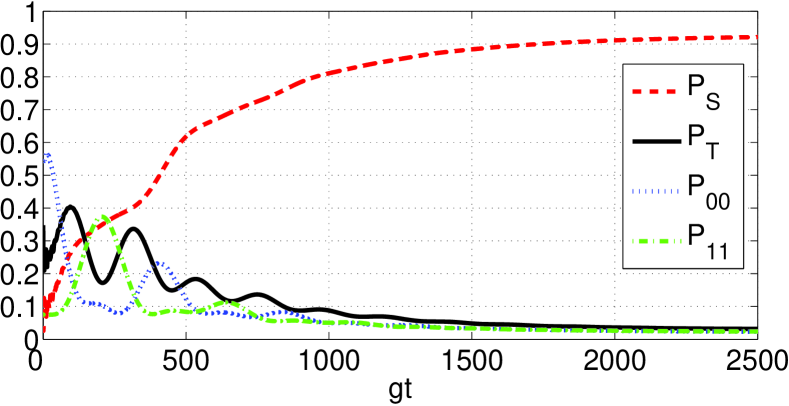
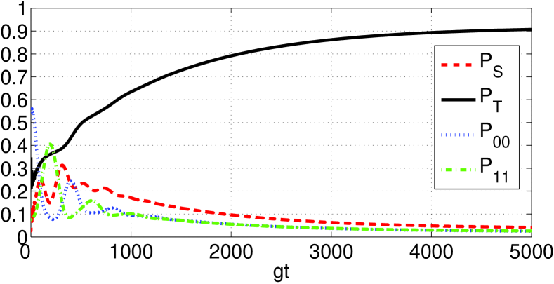
Figure 3: (Color online) The populations of states $|S\rangle$, $|T\rangle$, $|00\rangle$, and $|11\rangle$ versus the dimensionless parameter $gt$ for a random initial state by solving the full master equation. The curves are both plotted for an appropriate set of parameters $C$ $=$ $150$, $\gamma$ $=$ $2\kappa$, $\kappa=0.0577g$, $\gamma=0.1154g$, $\Omega$ = $0.06g$, $\Omega_{M}$ $=$ $0.0138g$, $\Delta$ $=$ $1.3g$, $\nu$ $=$ $0.4528g$ and $\delta$ $=$ $0.2875g$. (a) $\theta_{M}$ $=$ $0$; (b) $\theta_{M}$ $=$ $\pi$.

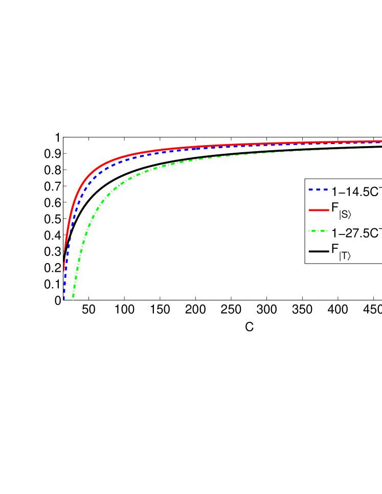
Figure 4: (Color online) The fidelity for steady-state entanglements $|S\rangle$ (red solid line) and $|T\rangle$ (black solid line) vs the cooperativity parameter $C$, and the mathematical fitting curves for maximizing $F_{|S\rangle}$ (blue dot line) and $F_{|T\rangle}$ (green dot dash line).

To evaluate the fidelity of the steady-state $|S\rangle$ or $|T\rangle$, we apply the rate equation as follows

$$\dot{P}_{S} = \kappa_{c_{1}}^{1}P_{00}-\big{(}\kappa_{c_{1}}^{2}+\gamma_{S}^{1,2}+\gamma_{S}^{3,4}\big{)}P_{S},$$ (40)

$$\dot{P}_{T} = \big{(}\kappa_{c_{2}}^{1}+\kappa_{c_{3}}^{1}\big{)}P_{00}$$ (42)

$$-\big{(}\kappa_{c_{2}}^{2}+\kappa_{c_{3}}^{2}+\gamma_{T}^{1,2}+\gamma_{T}^{3,4}\big{)}P_{T},$$

where $P_{\varphi}$ is the probability to be in the state $|\varphi\rangle$. When the whole system reaches the steady entanglement $|\varphi\rangle$, we assume $P_{\varphi}$ $\simeq$ $1$ and the probability in each of the other three states is nearly $P_{00}$, then $1-F_{|B\rangle}$ $\approx$ $3P_{00}$ ($B$ $=$ $S$, $T$). Here, $F_{|B\rangle}$ $=$ $|\langle B|\rho|B\rangle|$ is the fidelity of state $B$, and

$$1-F_{|S\rangle} \approx [\frac{3g_{e}^{2}\kappa}{8(C_{1}^{2}+D_{1}^{2})}+\frac{9\gamma_{e}}{32}]\big{/}[\frac{(\delta^{2}-2\nu^{2})^{2}g_{e}^{2}\kappa}{4B^{2}}],$$ (43)

$$1-F_{|T\rangle} \approx [\frac{3(\delta^{2}+2\nu^{2})g_{e}^{2}\kappa}{8(C_{2}^{2}+D_{2}^{2})}+\frac{9\gamma_{e}}{32}]\big{/}[\frac{\delta^{2}(\delta^{2}+2\nu^{2})g_{e}^{2}\kappa}{4B^{2}}].$$ (46)

We plot the fidelity for entangled steady-states with the cooperativity parameter $C$ and gain a simplified formula through mathematical fitting based on the least squares algorithm in Fig. 4, and find out the actual constants for maximizing the fidelity as follows

$$1-F_{|S\rangle} \simeq 14.5C^{-1},$$ (49)

$$1-F_{|T\rangle} \simeq 27.5C^{-1}.$$ (50)

The fidelities of the steady-state versus the fluctuations of coherent driving $\Omega$ and microwave $\Omega_{M}$ are plotted with full master equation in Figs. 5(a) and 5(b), and the results shows that the fidelity $F_{|S\rangle}$ and $F_{|T\rangle}$ remain higher than $91\%$ even when the relative errors in $\Omega$ and $\Omega_{M}$ reach $20\%$.

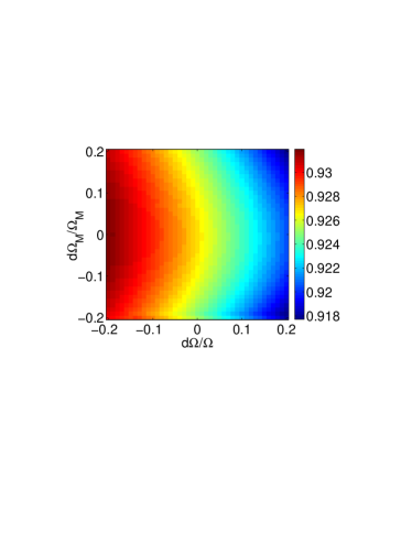
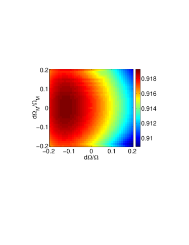
Figure 5: (Color online) Fidelity of the steady states versus the fluctuations of $\Omega$ and $\Omega_{M}$. $d\Omega$ and $d\Omega_{M}$ are the corresponding deviations of $\Omega$ and $\Omega_{M}$, respectively. Both plots are calculated with full master equation at time $t$ $=$ $9000$. (a) $F_{|S\rangle}$ vs $d\Omega/\Omega$ and $d\Omega_{M}/\Omega_{M}$; (b) $F_{|T\rangle}$ vs $d\Omega/\Omega$ and $d\Omega_{M}/\Omega_{M}$.

4 Influences of the dispersive mediating bosonic modes

In the above derivations, we assume that only one resonant mediating mode interacts with the cavity modes. We now consider the effects on the steady-state entanglement of other existing dispersive bosonic modes. Fig. 6 shows influences of the number $N$ of the mediating modes and the frequency spacing $\Delta_{x}$ on the fidelity $|F\rangle_{S}$.

$F_{|T\rangle}$ is influenced severely by the dispersive mediating modes and it is difficult to obtain the steady-state $|T\rangle$ when $N$ becomes large. Therefore, we just discuss the state $|S\rangle$ as follows. We first consider the case that two mediating modes are involved in Fig. 6(a), where we assume the first mediating mode is resonant with the cavity modes. There is a dip when $\Delta_{x}$ $=$ $-0.64g$. This can be explained as follows. The coupling between the mediating modes and cavity modes leads to frequency shifts of the delocalized field modes. When one of the delocalized modes, together with the classical laser field happens to induce the resonant Raman transition between two ground states ($|0\rangle$ and $|1\rangle$), as shown in Fig. 7, the Raman process, together with cavity decay, leads to effective decay $|0\rangle$ $\rightarrow$ $|1\rangle$ and destroys the entanglement.

The fidelity versus frequency spacing with three (five) mediating modes is plotted in Fig. 6(b) ( Fig. 6(c) ), showing that two valleys appear when $\Delta_{x}$ $=$ $-0.54g$ ($-0.58g$) and $\Delta_{x}$ $=$ $0.54g$ ($0.58g$). The appearance of two symmetric valleys in Fig. 6(b) ( Fig. 6(c) ) is due to the fact that two (four) equally spaced mediating modes are symmetrically distributed in two sides of the resonant mode. Especially, two small valleys appear when $|\Delta_{x}|$ $=$ $0.20g$ in Fig. 6(c), where two of those delocalized field modes are degenerate.

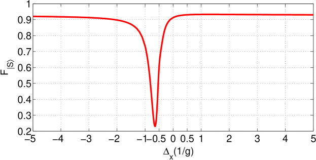
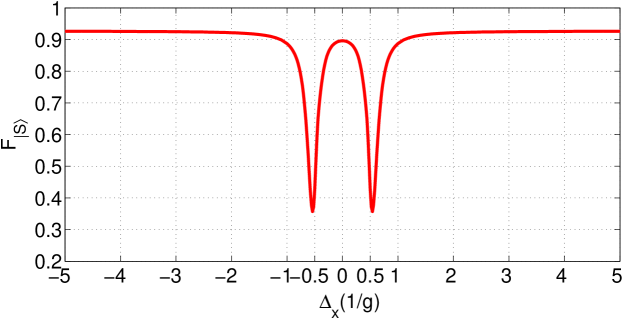
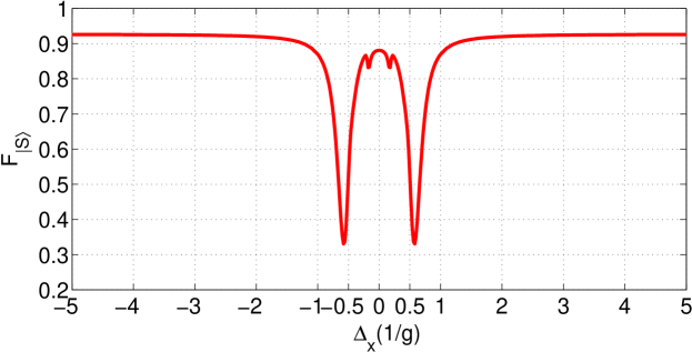
Figure 6: (Color online) Fidelity versus frequency spacing of the mediating bosonic modes. The parameters are the same as those in Fig. 3: (a) $N=2$; (b) $N=3$; (c) $N=5$.

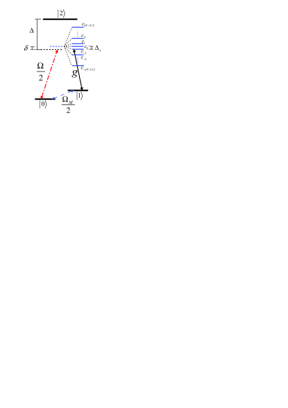
Figure 7: (Color online) The effective atom-field coupling when $N$ mediating modes are involved. The couplings between two cavity modes and $N$ mediating modes lead to $N+2$ delocalized field modes (blue solid line) with different frequency spacings, which interact with two atoms respectively. $c_{0}$ is the delocalized field mode resonant with the cavity modes. $c_{1}$ and $c_{-1}$ are the neighboring modes nearest to $c_{0}$, while $c_{-(N-1)/2}$, …, $c_{-2}$ and $c_{2}$, …, $c_{(N-1)/2}$ are other delocalized field modes.

Numerical simulations show that the fidelity of the steady-state entanglement is free from the effects caused by dispersive mediating modes when $\Delta_{x}$ $>$ $\delta$. Strong coupling for photons between distant nanocavities mediated by a waveguide at room temperature has been reported and the system dynamic control can be realized [42]. The cooperativity parameter $C$ about $100$ has been realized [43]. Based on these experimental techniques, the present scheme is feasible.

5 Conclusions

In summary, we have proposed a dissipation based scheme by which two atoms trapped in two distant cavities can be driven to steady-state entanglement. The competition based on the unitary dynamics and the dissipative dynamics leads to the entangled steady-state. Our results show that the dissipative mediating bosonic mode can be used as an entanglement catalyst for two distant atoms. The effects of dispersive mediating modes are analyzed. It is shown that the entanglement is robust against the fluctuations of the Rabi frequencies of the classical fields. We show that the distributed steady-state entanglements can be obtained with high fidelity regardless of the initial state and there is a linear relation in the scaling of the fidelity with the cooperativity parameter.

L.T.S., X.Y.C., H.Z.W. and S.B.Z. acknowledge support from the Major State Basic Research Development Program of China under Grant No. 2012CB921601, National Natural Science Foundation of China under Grant No. 10974028, the Doctoral Foundation of the Ministry of Education of China under Grant No. 20093514110009, and the Natural Science Foundation of Fujian Province under Grant No. 2009J06002. Z.B.Y acknowledges support from the National Basic Research Program of China under Grants No. 2011CB921200 and No. 2011CBA00200, and the China Postdoctoral Science Foundation under Grant No. 20110490828.

References

- [1] \NameSørensen A. S. Mølmer K. \REVIEWPhys. Rev. Lett.912003097905.
- [2] \NameZheng S. B. Guo G. C. \REVIEWPhys. Rev. Lett.8520002392.
- [3] \NameBeige A. et al. \REVIEWPhys. Rev. Lett.8520001762.
- [4] \NameLambrecht A. et al. \REVIEWAppl. Phys. B601995129.
- [5] \NameSimon C. Irvine W. T. M. \REVIEWPhys. Rev. Lett.912003110405.
- [6] \NameSerafini A., Mancini S., Bose S. \REVIEWPhys. Rev. Lett.962006010503.
- [7] \NameYang Z. B. et al. \REVIEWJ. Phys. B432010085506.
- [8] \NameYin Z. Q. Li F. L. \REVIEWPhys. Rev. A752007012324.
- [9] \NameSong J. et al. \REVIEWEur. Phys. J. D50200891.
- [10] \NameZheng S. B., Yang C. P., Nori F. \REVIEWPhys. Rev. A822010042327.
- [11] \NameYe S. Y.et al. \REVIEWPhys. Rev. A822010012307.
- [12] \NameOgden C. D. et al. \REVIEWPhys. Rev. A782008063805.
- [13] \NameHartmann M. J. et al. \REVIEWLaser Photon. Rev.22008527.
- [14] \NameYang Z. B. et al. \REVIEWEur. Phys. J. D612011737.
- [15] \NameKastoryano M. J., Reiter F., Sørensen A. S. \REVIEWPhys. Rev. Lett.1062011090502.
- [16] \NameReiter F., Kastoryano M. J., Sørensen A. S. \REVIEWNew J. Phys.142012053022.
- [17] \NameReiter F. Sørensen A. S. \REVIEWPhys. Rev. A852012032111.
- [18] \NameShen L. T. et al. \REVIEWPhys. Rev. A842011064302.
- [19] \NameBusch J. et al. \REVIEWPhys. Rev. A842011022316.
- [20] \NameCho J., Bose S., Kim M. S. \REVIEWPhys. Rev. Lett.1062011020504.
- [21] \NameMemarzadeh L. Mancini S. \REVIEWPhys. Rev. A832011042329.
- [22] \NameVollbrecht K. G. H., Muschik C. A., Cirac J. I. \REVIEWPhys. Rev. Lett.1072011120502.
- [23] \NameAlharbi A. F. Ficek Z. \REVIEWPhys. Rev. A822010054103.
- [24] \NameWang X. T. Schirmer S. G. arXiv:1005.2114v2
- [25] \NameBenatti F., Floreanini R., Piani M. \REVIEWPhys. Rev. Lett.912003070402.
- [26] \NameChen X. Y. et al. \REVIEWJ. Opt. Soc. Am. B2920121535.
- [27] \NameRafiee M. et al. \REVIEWPhys. Rev. A852012042320.
- [28] \NameValle E. D. \REVIEWJ. Opt. Soc. Am. B282011228.
- [29] \NameYang W. L. et al. \REVIEWPhys. Rev. A852012022324.
- [30] \NameAngelakis D. G. et al. \REVIEWEur. Phys. Lett.85200920007.
- [31] \NameBraun D. \REVIEWPhys. Rev. A892002277901.
- [32] \NameLiu K. L. Goan H. S. \REVIEWPhys. Rev. A762007022312.
- [33] \NameChou C. H. et al. \REVIEWPhys. Rev. E772008011112.
- [34] \NameHorhammer C. Buttner H. \REVIEWPhys. Rev. A772008042305.
- [35] \NamePaz J. P. Roncaglia A. J. \REVIEWPhys. Rev. Lett.1002008220401.
- [36] \NameLi P. B. et al. \REVIEWPhys. Rev. A852012042306.
- [37] \NameMessina R. et al. \REVIEWPhys. Rev. A802009022119.
- [38] \NameKrauter H. et al. \REVIEWPhys. Rev. Lett.1072011080503.
- [39] \NameTan S. M. et al. \REVIEWPhys. Rev. Lett.661991252.
- [40] \NameHillery M. et al. \REVIEWPhys. Rev. A5919991829.
- [41] \NameCirac J. I. et al. \REVIEWPhys. Rev. Lett.7819973221.
- [42] \NameSato Y. et al. \REVIEWNature Photon.6201156.
- [43] \NameHennessy K. et al. \REVIEWNature Photon.4452007896.