Genetic flow directionality and geographical segregation in a Cymodocea nodosa genetic diversity network

Abstract

We analyse a large data set of genetic markers obtained from populations of Cymodocea nodosa, a marine plant occurring from the East Mediterranean to the Iberian-African coasts in the Atlantic Ocean. We fully develop and test a recently introduced methodology to infer the directionality of gene flow based on the concept of geographical segregation. Using the Jensen-Shannon divergence, we are able to extract a directed network of gene flow describing the evolutionary patterns of Cymodocea nodosa. In particular we recover the genetic segregation that the marine plant underwent during its evolution. The results are confirmed by natural evidence and are consistent with an independent cross analysis.

Introduction

With the advances of sequencing technology and the availability of large datasets, evolutionary biology needs to employ novel techniques, which are akin to those developed within statistical physics [1], to analyse and understand patterns in population dynamics. An interesting question in evolutionary biology is how to trace the directionality in migration patterns, a problem of outstanding importance in conservation biology in general, including the management of threatened or exploited species and of invasion processes [2]. It is also related to the more general problems of infection and information propagation in networks [3, 4].

In this paper we tackle the indirect assessment of migratory transfers (by pollen, propagules, or plant fragments) among plant populations using molecular markers to retrace the exchange of genes, or gene flow, among them. This is done by fully developing a recently introduced methodology based on a directionality index [5]. This index finds its origins on the concept of geographical segregation [6], often related to social studies, to infer the evolutionary pathways from microsatellite datasets. Microsatellites [7] are portions of non-coding DNA with a variable number of repetitions of a motif consisting of a few bases. They are widely used in intraspecific genetic studies. Despite being non-coding, we will use eventually the word genes to denote the microsatellites, and alleles for their different varieties occurring at a particular position in the genome (a particular locus).

Classical population genetics analyses do not allow inferring the direction of migration using molecular data. Although some Bayesian analyses have been more recently developed to do so [8, 9], many require complex and time-consuming computing of the likelihood functions, restraining the ability to explore more than often too simple evolutionary scenarios and molecular models [10].

In the present study we analyse a dataset that presents evident cases of geographical segregation, such as island effects and we are able to show that the proposed methodology spots these islands, based on microsatellite data only and without any further geographical information or evolutionary assumption. In particular we use the information contained in microsatellite genetic markers from the entire geographic distribution of a marine plant species, Cymodocea nodosa (CN). This dataset has been selected because there is enough information to infer the past history of the gene flow based on the geographical distribution of genetic polymorphism [11], allowing the assessment of the usefulness of the new methods here described.

Understanding the pathways of gene flow along the Mediterranean-Atlantic transition zone was the main aim of this genetic dataset [11]. Based on presence/absence of alleles, this revealed that the flow of genetic information across the Mediterranean-Atlantic transition zone had most likely occurred westwards, because dominant Mediterranean alleles penetrate into the nearest Atlantic sites (Atlantic Iberia), but the opposite is not true, i.e. dominant Atlantic alleles are not found in any Mediterranean populations. This clear pattern of presence/absence of diagnostic alleles results in that this data set provides an ideal workbench to test and to develop a recently introduced method of inferring directionality of gene flow, here based on distances computed from the Jensen-Shannon divergence [12].

Network theory has already proved to be useful in the study of metapopulation systems dynamics [13]. In particular it has been shown that the analysis of topological relationships between different populations carries fundamental information for the understanding of evolutionary dynamics [13]. It is important to further develop and test methodologies to extract reliable information-flow networks from biological datasets.

The method considered in this work introduces some novelties with respect to classical approaches, that have been already underlined in [5]. The gene flow network is extracted by means of a model-independent measure, that is a normalised version of the Jensen-Shannon divergence. An interesting aspect of the application of this method is that we extract the gamete space from the allele sequences and we perform the analysis in that space. Gametes are the mother and father sexual cells that fuse in a sexual reproduction event. The nuclear genetic information from the two gametes remain mostly separated in the daughter cell (in the different chromosomes of each chromosome pair) and subsequent cells originating from it, but sequencing techniques can not identify which gene is coming from which gamete. From the observed alleles in each individual in our dataset we construct the set of possible gametes that could have originated such individual, and we apply our techniques to such gamete pool. The distance measure in the gamete space has to be considered more detailed than the one in the allelic space, since it takes into account the possible correlations between different loci. An extension of the method to include mutation effects can be easily obtained as better explained below.

Here we advance the method beyond its first application [5], in fully developing and verifying the directionality index methodology by introducing a test for the detected directionality significance. This is done with an ad-hoc randomization test. This method is independent of the way the genetic flow is extracted and can then be applied independently of the genetic distance used. The present analysis reveals that the methodology is efficient in cases of evident geographical segregation, for which the method was designed, while it is not efficient in detecting the direction of the flows where geographical segregation is not present.

Moreover in the Additional file 1, we give a detailed comparison of the distance method applied here with some of the most used genetic distance measures based on microsatellite analysis, such as the Nei distance [14], the Cavalli-Sforza distance [15], the Goldstein distance [14] and the average square distance [16].

Data and results

The genetic flow network

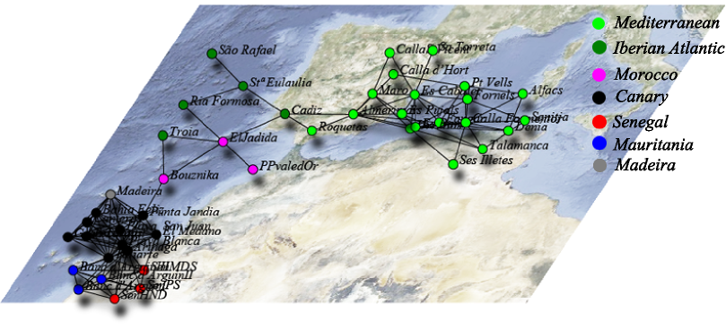
Figure 1: Figure 1 - Genetic flow network for Cymodocea nodosa. Genetic flow network for Cymodocea nodosa meadows at the percolation threshold, obtained via the JSD measure applied to raw gamete data from the sampled meadows (the genetically very distant and disconnected Greek populations are not shown). Different colors indicate the different meadow origins. The network is displayed via a spring embedding algorithm, i.e. it does not contain geographical information. Nevertheless the genetic clusters well trace the different geographical origins, as it is possible to see by comparison with the approximately overlayed map displayed below.

Our dataset consists of 845 ramets of CN. A ramet is a single plant shoot, whereas a genet is a genetic individual, or clone, derived from a single event of sexual recombination (i.e., from a single seed) and having given birth through clonal growth to a population of ramets therefore sharing the same genome [17]. Ramets were sampled from 60 different meadows, distributed geographically between the Mediterranean basin and the Atlantic Ocean, covering the entire plant distribution [11]. This dataset is the one discussed in [11] with the addition of a few populations more recently sampled, as for example from Morocco. Among the 40 ramets taken at each site, after removal of genet (i.e., clonal) repetitions the number of ramets available in the data set ranged from 4 to 34 per meadow. Hence each of the 845 ramets of the dataset represents a different clone.

We characterize each ramet by some microsatellite markers [7]. In particular, each ramet has been genotyped to identify in it $n=8$ pairs of alleles, i.e. pairs of microsatellites that occupy a specific position (locus) on the chromosomes, each element of the pair characterizing the same locus in the two homologous chromosomes arising from the maternal and paternal gametes in a sexual reproduction event. The number $n$ of pairs of microsatellites used was selected for highest information content with minimum cost ([11] and references therein), a standard microsatellite genotyping methodology.

To characterize the presence of gene flow between meadows we use the general network strategy [18, 13, 19], in which populations (here, the meadows) are nodes of a graph, and they are linked when significant relationships among them (indicating gene flow) are detected.

There are different ways to implement such inference of gene flow, mostly based on different types of distances [18, 13, 20]. Here we use a methodology based on information theory [5], which is especially suited to compare genetic data taken from populations of different sizes, taking into account not just properties of individual alleles but also the full information genotyped (including correlations among sites, linkage disequilibrium, for example).

We consider the set of meadows as a metapopulation system where each population is a meadow and each population element is a n-dimensional vector representing an equiprobable gamete of that meadow, where n is the number of loci.

To derive the gamete pool we notice that each ramet is characterised by a set of n=8 pairs (a,b) of alleles, each pair belonging to a given locus. Since it is not known a-priori which chromosome a given allele belongs to, we consider all the possible combinations of alleles between the n pairs, i.e. $2^{n}=256$ equiprobable gametes representing a single ramet. In this way our system becomes represented by $845\cdot 2^{8}=216320$ points in a 8-dimensional space. Each meadow can be characterised by a discrete probability function $P=P(\overrightarrow{x})$ assigning a relative weight to each of the possible gametes $\overrightarrow{x}$ in n-dimensional space, i.e. $P=P(\overrightarrow{x})$ is the probability to find the gamete $\overrightarrow{x}$ in that meadow.

For each pair of meadows characterised by probability distributions $P=P(\overrightarrow{x})$ and $Q=Q(\overrightarrow{x})$ we calculate the normalised Jensen-Shannon divergence

$$JSD(P\|Q)\equiv\frac{H(\pi_{A}P+\pi_{B}Q)-\pi_{A}H(P)-\pi_{B}H(Q)}{-\pi_{A}\ln\pi_{A}-\pi_{B}\ln\pi_{B}},$$ (1)

With $\pi_{A,B}=n_{A,B}/(n_{A}+n_{B})$, $n_{i}$ the sample size of meadow i and $H(F)=-\sum_{\overrightarrow{x}}F(\overrightarrow{x})\ln F(\overrightarrow{x})$ the Shannon index or entropy of distribution $F$.

The information-theoretic meaning of JSD is discussed in detail in [12, 21, 5]. We stress that JSD is a measure of difference between $P$ and $Q$ that takes into account the information on the gametes which are shared by both populations as well as the ones which are exclusive to one of them. This second capability is not present in other information-theoretic distances, such as the Kullback-Leibler divergence [12].

In the Additional file 1, we illustrate in detail the relationships between Eq. (1) and other classical measures to calculate genetic divergence. We want to stress that Eq. (1) is independent of any evolutionary assumption, i.e. it just calculates the punctual correlations within the meadows’ attribute probability distributions. Nevertheless it is possible to relax and extend such a measure to include mutation effects, just considering the computation of the probability distribution in a n-dimensional sphere of a given radius, surrounding the point $\overrightarrow{x}$. Varying such a radius, it is then possible to coarse-grain the system at different resolutions.

JSD distances are calculated among all pairs of meadows. Smaller distance implies stronger genetic identity among the meadows. By selecting a particular threshold value for the distance we can represent the genetic flow as a network [13, 5] in which meadows with smaller JSD distance appear linked. As we increase the threshold we observe how the different linked clusters of populations become larger and merge.

A convenient threshold to use is the percolation threshold [13], at which a connected path across the whole geographic area first appears. The network fragments for threshold values below the percolation threshold, while the genetic flow spanning the network remains robust above it. At this point different clusters, and subclusters, representing sets of meadows with important internal gene flow, and gene paths among them, can be identified.

In Fig. 1 we show the network at the percolation threshold, when the major components in the network connect. As we can see the purely topological genetic flow network accurately reflects the geographical locations to which the different meadows belong. There are well connected clusters representing Senegal, Mauritania, Canaries and Madeira, then we have the other large cluster spanning within the Mediterranean meadows. Between those two big clusters we find the Atlantic Iberian meadows and the Moroccan meadows.

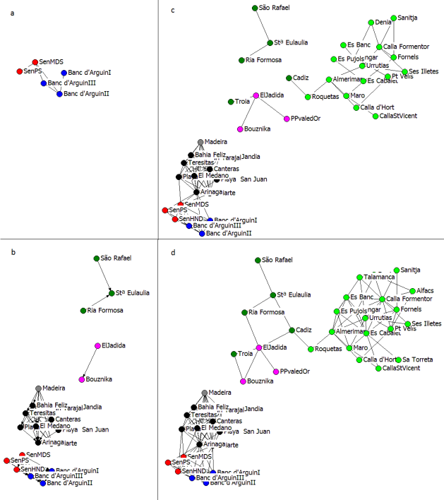
Figure 2: Figure 2 - Genetic flow network for Cymodocea nodosa at growing values of the distance threshold. Clusters that appear when linking populations with a JSD distance smaller than a distance threshold $T$, for increasing values of $T$ approaching from below the percolation threshold. a) $T=0.57$. b) $T=0.89$. c) $T=0.95$. d) $T=0.97$, just below the percolation threshold. The cluster colors are the same as in Fig.1.

While this representation is interesting to understand the effectiveness of JSD as a genetic divergence measure, it also confirms the findings of [11] regarding the main evolutionary scenario for CN. To see that we plot in Fig. 2 the connected clusters that form when increasing the distance threshold. We interpret that the first populations to merge when the genetic distance threshold is raised from zero are the ones that differentiated more recently. Then small genetic divergences correspond to the most recent time of divergence. In our analysis we observe that the first meadows to be connected are the ones South of the Canaries, while the ones that are more distant are the ones in Greece (those do not appear in the figure, since they are not connected until higher distance thresholds), with a range of intermediate distances in between. Then we can infer an evolutionary dynamics that starts in the Greek Sea, goes to the main Mediterranean basin and then spreads in the Atlantic. This coincides with the ancient history of habitat colonization by this species inferred in [11], which proposes that the species originated in the eastern Mediterranean by divergence from its close relative in the Indian Ocean/Red Sea and colonized the western Mediterranean and Atlantic by spreading westwards. Moreover the fact that Senegal and Mauritania cluster strongly with the Canaries and Madeira, in respect to the weak clustering of the Canaries with Morocco and the Iberian Atlantic, is in agreement with the evolutionary scenario previously suggested on the basis of biogeographical information. These findings are also in agreement with the possible extinction of meadows in Morocco and Iberia during the last glacial maximum, that was accompanied by a drop in sea surface temperatures below the range at which CN commonly occurs, and by a drop of sea level that changed coastline morphology [22], that would have been followed by colonization of this region by an admixture of Atlantic and Mediterranean genetic types [11].

Inferring genetic flow directionality

The second part of the analysis is about inferring the directionality of the detected gene flows. The main question we pose is: “is it possible to understand which is the source and which the sink in a given genetic channel?”. To understand this, we further develop the technique introduced in [5] based on geographical segregation [6]. We say that a population is segregated when it contains elements (gametes in our case, but this could equally be applied to alleles, as shown in the Additional file 1) quite exclusive and distinct from the rest of populations, and elements common in other populations are not so abundant here. The main reasoning resides on the observation that a population which is initially segregated will not maintain its character if it is open to receive gametes from other different ones. It will remain segregated only if there is no gene exchange or if there is some but the population acts as a source.

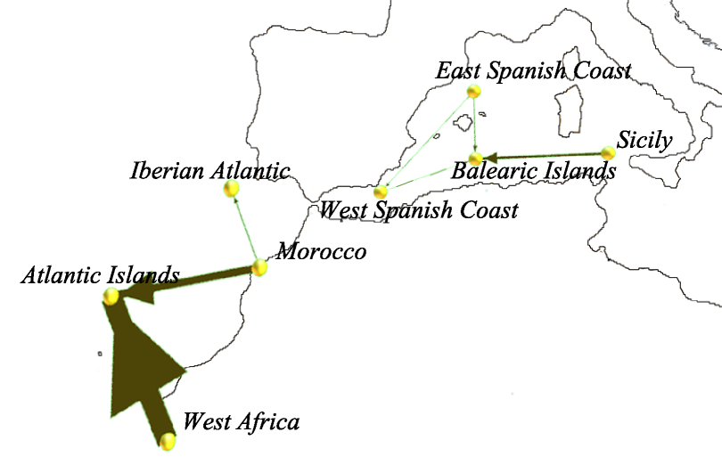
Figure 3: Figure 3 - Gene flow directionality network. Gene flow directionality network for Cymodocea nodosa genetic flow network evaluated in the gamete space. Nodes represent populations of meadows grouped together by their geographical attributes. Arrows are directional genetic flows, their width is proportional to the value of R, quantifying the significance of the inferred directionality.

In terms of frequency distributions, these are peaked on particular elements in segregated populations, whereas distributions are more unstructured in those acting as sinks receiving genes from different sources. Between any pair of populations among which a genetic flow has been detected (as described in the previous section, this occurs when their genetic distance is smaller than the given percolation threshold), a directionality index $I_{PQ}$ is defined between meadows characterized by gamete distributions P and Q. It takes into account the different segregation state of the pairs of populations by means of the respective Shannon information indices, corrected for their different sizes and number of common elements.

To be more precise, given the two populations characterized by $P$ and $Q$ let us denote by $D_{P}$ the set of different gametes present in the first population, $D_{Q}$ the ones present in the second, $X=D_{P}\bigcup D_{Q}$ the total set between both populations, and $J=D_{P}\bigcap D_{Q}$ the set of common gametes (that we assume to be non-empty). We denote by $\mu_{P}$ the fraction between the number of gametes common to both populations with respect to the total number of gametes in the first one, and analogously we define $\mu_{Q}$ as the fraction of common gametes between both populations with respect to the total number of gametes in the second one. We have $0<\mu_{P,Q}\leq 1$ and if $\mu_{P}$ or $\mu_{Q}$ is close to one, it means that the shared alleles are the dominant part of the corresponding population. Let us denote by $P_{J}=P_{J}(\overrightarrow{x})$, with $\overrightarrow{x}\in J$, the frequency distribution of the alleles in the first population, normalized to unity when summing over all the common alleles (the $J$ set), and analogously we define $Q_{J}=Q_{J}(\overrightarrow{x})$, with $\overrightarrow{x}\in J$.

With these definitions, the directionality index is defined as [5]:

$$I_{PQ}\equiv-{\rm sign}\left[\frac{H(P_{J})}{\mu_{P}}-\frac{H(Q_{J})}{\mu_{Q}}\right]$$ (2)

where H is the Shannon index of the distributions, as defined in the previous subsection.

If $I_{PQ}=1$ we can infer a direction of the genetic flow from the first to the second population, whereas $I_{PQ}=-1$ indicates the reverse flow. The idea is that the net flow of gametes is from the less entropic (i.e., less diverse, more segregated) populations towards the more entropic, properly adjusting for the different sizes and fraction of common alleles. Very diverse populations can not be sources of only very specific gametes, and they are more likely to be sinks, whereas the reverse will be true for segregated populations. Large width of gamete distributions may be an indicator of large diversity, but it is better to use the Shannon information as a more robust indicator of diversity. For more information about our directionality indicator we refer to [5].

Significance test of the detected directions

The idea of tracing the directionality of gene flow via a measure of geographical segregation turns out to be a delicate point. First of all this method is applicable in case there are traces of segregation in the subset of shared gametes of the considered meadow. After that we have to understand if the difference in the segregation indexes between the two meadows in consideration is large enough to let us infer a direction for the genetic flow.

To address these points first we should remember that the data set used to infer directionality is not the whole set of gametes, as used for network construction, but just those gametes that are shared by the two samples in consideration. A convenient way to quantify the number of shared gametes is by means of the proportion $\mu_{P}$ of shared gametes between populations characterized by distributions P and Q, with respect to the total number of gametes in the population characterized by P. We emphasize that $\mu_{P}$ is not only a property of population P, but of the pair of populations being compared. This proportion should be non-negligible in order to infer reliable conclusions for the flow directionality.

Second, to understand if the detected directionality $I_{PQ}$ between two meadows of size $n_{1}$ and $n_{2}$ is a sign of segregation or it is a random effect, we first measure the magnitude for the directionality index $I_{PQ}$ and then we measure it again after having shuffled the sample. To shuffle the sample we consider two meadows of size $n_{1}$ and $n_{2}$ and we fill them randomly with the genets extracted from the original two meadows. We repeat this operation 1000 times, so to obtain an estimation of the distribution for the randomised directionality index, which turns out to be Gaussian. From there one gets the average randomised directionality index $I_{PQ}^{R}$ and its standard deviation $\sigma_{R}$.

The ratio $R=|I_{PQ}-I_{PQ}^{R}|/\sigma_{R}$ gives us the number of standard deviations (sd) the measured segregation index is far from the expected one in a random situation. For instance obtaining a value of R larger than 2.58 has a probability $p<0.01$ of being explained by randomness.

Randomisation test
Link P-Q	R	$\mu_{P}$	$\mu_{Q}$
WA-AI	442.48	0.26	0.01
MO-AI	159.16	0.03	0.004
SI-BI	65.45	0.02	0.008
ESC-BI	15.64	0.17	0.06
SI-BI	65.45	0.02	0.008
MO-IA	13.61	0.07	0.03
ESC-WSC	4.92	0.09	0.07
WSC-BI	4.4	0.24	0.13

Table 1: Results of the randomisation test for the directionality analysis. Only the significant ($p<0.01$) directionalities are listed. In the first column the population pairs, in the second column the value of $R$ calculated over 1000 replicas, in the third column $\mu_{P}$, in the fourth column $\mu_{Q}$. The acronyms stand for: WA: West African coast, AI: Atlantic islands, MO: Morocco, SI: Sicily, BI: Balearic Islands, ESC: East Spanish coast, IA: Iberian Atlantic, WSC: West Spanish coast.

Results

To have a better statistical sample, we group the elements of the clusters shown in Fig. 1 into single populations. Since we are interested in retrieving the directionalities of gene flow, we cluster the meadows according to their geographical origin. Nevertheless such a clustering is not significatively different from the one that would be obtained via a technique based, for example, on modularity minimisation [23].

In Fig.3 we show the results for the directional analysis. The widths of the arrows are proportional to $R$, quantifying the significance of the relationship. The genetic flow directionality traces are found to be significant in terms of $R$ and $\mu$ (see Tab. 1) from the Spanish Coast and Sicily to the Balearic Islands, from the African coast to the Canary Islands and Madeira, from the East (Mediterranean) Spanish Coast to the West (Mediterranean) Spanish Coast and from Morocco to the Iberian Atlantic. These results agree with expectations from inferences based on allele presence/absence by [11] and [24].

These results tell us that the method correctly identifies phenomena of geographical segregation. This phenomenon is typical for islands, where it is not easy for species to genetically mix with far away populations. Then we can see that all the islands in the studied sample are identified as sinks of the genetic flow. Also the main east toward west spread trend has been identified by this methodology.

In contrast with the recent events of gene flow, this method is not efficacious to trace the directionality from the Mediterranean basin to the Atlantic, a much more ancient process that took place before all the glacial range shifts and post-glacial recolonization migrations, since there is no trace of segregation in that case. Directionality of the genetic flow, at such ancient scales, cannot be spotted with this technique.

Discussion

The directional network resulting from this analysis is in agreement with diverse and converging information on historical fluctuation of species ranges along the Mediterranean-Atlantic transition zone, associated to paleoclimatic events, putative recolonization pathways and secondary contact zones inferred from biogeographic analysis on various taxa, and expectation derived from oceanographic modeling.

The directed network (Fig. 3) reveals a clear trend of gene flow of South-Western preferential migration pathways from the Western and central Mediterranean meadows towards the Almeria-Oran front (an oceanographic feature east of the Gibraltar strait). This coincides with the gene flow paths that were previously hypothesized on the basis of many private alleles found in the Atlantic that do not enter this transition zone, whereas Mediterranean polymorphism was much more shared with populations from the transition zones [11]. Modeled Lagrangian dispersal trajectories across the East-West Mediterranean divide [25]) from March to June, the fruit dispersal season for Posidonia oceanica (which flowers in the winter), support a main trend of particle exchange toward West in the Mediterranean [26]. This was associated to a lack of dispersal expected toward Sicily and the Eastern part of the Mediterranean, as predicted from the prevailing current directions. Despite having a different reproductive season (flowering in spring, seeds produced in summer) and seeds that develop buried in the sediment and are not expected to disperse with currents, CN is likely to disperse via reproductive plant fragments, drifting along these same current directions, in agreement with the inferences of the present directionality flow network analysis, from Sicily westwards.

Besides this direction of the Mediterranean flow toward the Almeria-Oran populations, a second major result with the presented methodology is the confirmed lack of input of the Atlantic into the Mediterranean. Preferential pathways of migration within the Atlantic show strong directionality of flow from Western Africa and Morocco toward the Canary islands, and from Morocco toward Iberian Atlantic populations of the transition zone, with no sign of any entrance of Atlantic flow into the Mediterranean.

In summary, the directed network built here confirms a dominant direction of fluxes with a East-West direction in the Mediterranean from Sicily and Spain toward South Western meadows and Almeria-Oran Front, and the lack of mirror exchange from the Atlantic toward the Mediterranean.

A phenomenon that can confound some of our techniques is that of a genetic bottleneck. This consists of a large reduction of population size, which leads also to a much decreased diversity because of genetic drift[27]. This happens for example if only a few individuals colonize a new island (founder effect) and expand there. The recovered new population has small diversity, with the potential to be identified as a “source” although in fact it has been the receiver of the gene flow. Fortunately this is not a problem because our methodology does not compute the directionality index for all pairs of populations, but only among those whith a strong similarity, as measured by the JSD distance. Our measure of genetic flow will give a very small value in the case mentioned above. In addition, even if a recent and strong bottleneck (i.e. contemporary to the sampling) or a recent re-expansion post-bottleneck may transitorily induce “source-like” characteristics in the distributions, such distributions would display a characteristic lack of polymorphism in the first case, and a typical genetic signature on the distribution of polymorphism and divergence in the latter that will be easily detected by available population genetics tools [28, 29]. A careful examination of data should thus allow discarding such confounding factor or pointing it as a possible alternative explanation of directionally detected with our methods.

We stress that the data treatment presented in this paper is independent of evolutionary assumptions, but that it can be easily extended to include mutation. This can be done, as we already point out, coarse-graining the probability space in function of a simple parameter indicating the resolution with which we distinguish different gametes. Then varying this parameter it is possible to study the evolutionary paths at different time windows, but further research in this direction is needed to better implement these points.

While the present research is about genetic flow dynamics, the whole information flow/directionality index method has a wider range of application, from metapopulation systems to social dynamics and more in general it can be relevant whenever a given population can be represented by vectors of attributes in a symbolic space.

Competing interests

The authors declare that they have no competing interests.

Author’s contributions

PM developed the methodology and performed the analyses. SAH and EAS provided the data and the biological interpretations. VME and EHG contributed to the methods and to the analyses. All authors participated in the writing of the paper.

Additional file 1

Here we compare $JSD$ as defined in Eq.1 of the main text with some of the most used genetic distances. In particular we compare it with the Nei distance $NEI$ [15], the Cavalli-Sforza distance $CS$ [30], the Goldstein distance $GD$ [16] and the average square distance $ASD$ [14]. $D$, $NEI$ and $CS$ are distances defined in a symbolic space, while $GD$ and $ASD$ are defined in metrical space where the metric is defined by the allele repetitions.

The Cavalli-Sforza distance $CS$ is defined as

$$CS=\sqrt{4\frac{\sum_{l}(1-\sum_{i}\sqrt{x_{i}y_{i}})}{\sum_{l}(a_{m}-1)}}.$$ (3)

Here $x_{i}$ is the fraction of allele $i$ in the first population, $y_{i}$ is the fraction of allele $i$ in the second population. A second sum is over the loci $l$ and $a_{m}$ is the total number of alleles, but if we work in the gamete space, then $x_{i}$ and $y_{i}$ refer to gamete frequencies and $l=1$.

$NEI$ is defined as:

$$NEI\equiv-\log\left(\frac{\sum_{l}\sum_{i}x_{i}y_{i}}{\sqrt{\sum_{l}\sum_{i}x_{i}^{2}\sum_{l}\sum_{i}y_{i}^{2}}}\right).$$ (4)

The main statistical difference between $NEI$ and $CS$ with $JSD$, as we are going to show, is that $JSD$ incorporates a weighting system for the different population sizes, while $NEI$ and $CS$ don’t.

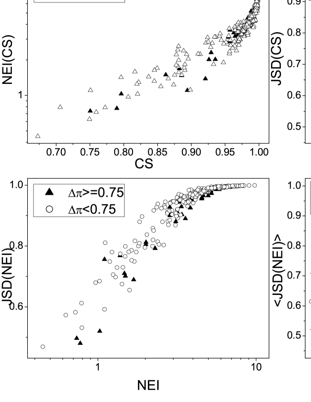
Figure 4: Measures performed for the CN dataset. Top-left: correlations between $NEI$ and $CS$. Top-right: $JSD$ versus $CS$. Bottom-left: $JSD$ versus $NEI$. Bottom-right: $<JSD(NEI)>$ versus $NEI$.

In Fig.1 we show the correlations between those measures, as measured in the CN dataset. For a reason that will be clear below we define the parameter $\Delta\pi=|\pi_{1}-\pi_{2}|$ as the absolute value of the difference of the statistical weight between population 1 and 2. We represent with black triangles the distances between populations whose weight difference $\Delta\pi$ is larger or equal than 0.75 and with white circles the distances between those populations whose weight difference $\Delta\pi$ is less than 0.75.

In the top-left panel we show the plot for $NEI$ versus $CS$. The main difference between $NEI$ and $CS$ is that $NEI$ considers the variance of the gamete distributions, while $CS$ doesn’t. We see that the measures are well correlated with the differences given by the variances of the populations.

In the top-right panel we show the plot of $JSD$ versus $CS$. Also in this case the measures are positively correlated, even if two different branches appear in the plot. Those two branches appear to be well represented by the two different categories for $\Delta\pi$. In fact when the population sizes are very different, $\Delta\pi\geq 0.75$, we see that $CS$ overestimates the distance between them in respect to $JSD$.

In the bottom-left panel we show the plot of $JSD$ versus $NEI$. Again we can see that the measures are well correlated, but also in this case $NEI$ overestimates the distance between two populations when $\Delta\pi\geq 0.75$, even if this is less evident that in the previous case. Nevertheless if we look at the plot of the average value of the $JSD$ corresponding to the same $NEI$, $<JSD(NEI)>$, on the bottom-right panel, we can see that it is true in average, since each black triangle is below the correspondent white circle.

The average square distance $ASD$ between population $A$ and $B$ is defined as [14]:

$$ASD_{k}\equiv\sum_{i,j}(i-j)^{2}f_{i}f_{j}=(\mu_{A}^{k}-\mu_{B}^{k})^{2}+V_{A}^{k}+V_{B}^{k}=(\delta\mu^{k})^{2}+V_{A}^{k}+V_{B}^{k},$$ (5)

where $i$, $j$ are the repetition numbers of allele $i\epsilon A$ and $j\epsilon B$ and $f_{i,j}$ its frequency at locus $k$. Then $\mu_{X}^{k}=\sum i\cdot f_{i}$ is the average repetition number at locus $k$ for population $X$ and $V_{X}^{k}=\sum f_{i}(i-\mu_{X}^{k})$ is the variance in the repetition number of population $X$ at locus $k$. Eq.5 has to be averaged on the loci then.

$$ASD=\frac{\sum_{l}^{n}ASD_{k}}{l}.$$ (6)

The Goldstein distance $GD$ between two populations $A$ and $B$ defined by a set of alleles is defined at the locus $k$ as [16]:

$$(\delta\mu^{k})^{2}\equiv(\mu_{A}^{k}-\mu_{B}^{k})^{2},$$ (7)

where $\mu_{X}^{k}$ is the average number of repetitions for population $X$ at locus $k$.

In the case of $n$ different loci Eq.7 is averaged on the different loci:

$$GD\equiv\frac{\sum_{k=1}^{n}(\delta\mu^{k})^{2}}{n}.$$ (8)

$GD$ was introduced as an improvement of $ASD$ ”because distances based on the infinite-alleles model are nearly linear with time immediately following isolation, it is not worthwhile to use $ASD$ with very closely related groups” [16].

The difference between $GD$ and $ASD$, as it is clear from Eq.5 and Eq.8, resides on the presence in $ASD$ of the variance of the attributes.

To understand the difference between $JSD$ and $GD$ in the gamete space, we have to keep in mind the representation of the genet in the gamete space as explained in the main paper. The gamete space is a $n$-dimensional space, each dimension representing a locus, where a diploid genet is represented by a set of $2^{n}$ points. For a population $X$ such a distribution of points has a centre of mass, whose coordinates $\mu_{X}^{k}$ ($k=1,..,n$) are given by the average repetition number for each locus $\mu_{X}^{k}=\sum i\cdot f_{i}$. Hence, given two populations $A$ and $B$, the distance between their average point in the attribute space is given by $\sqrt{\sum_{i=k}^{n}(\mu_{A}^{k}-\mu_{B}^{k})^{2}}=\sqrt{n\cdot GD}$ (see Eq.8).

Figure 5: Measures performed for the CN dataset. Left panel: $JSD$ versus $GD$. Right panel: $JSD$ versus $ASD$

Hence $GD$ is the square root of the distance between the centre of mass of the populations as represented in the gamete space. $JSD$ instead is a punctual information measure that considers all the point correlations between the two populations. Then $JSD$ and $GD$ could be correlated, this does not occur always. For instance there is an extreme case where population $A$ and $B$ have the same centre of mass in the gamete space, so that $GD=0$, but not a single common gamete so that $JSD=1$. We can observe this in Fig.2, where we show evidence for not very strong correlations between $JSD$ and $GD$ in the left panel and between $JSD$ and $ASD$ in the right panel, as measured for the CN dataset.

References

- [1] Drossel B: Biological evolution and statistical physics. Adv Phys 2001, 50(2):209–295.
- [2] Travis J, Park K: Spatial structure and the control of invasive alien species. Anim Conservation 2004, 7:321–330.
- [3] Haydon D, Cleaveland S, Taylor L, Laurenson M: Identifying reservoirs of infection: A conceptual and practical challenge. Emerging Inf Dis 2002, 8:1468–1473.
- [4] Vespignani A: Modelling dynamical processes in complex socio-technical systems. Nature Physics 2012, 8:32–39.
- [5] Masucci AP, Kalampokis A, Eguíluz VM, Hernández-García E: Extracting directed information flow networks: An application to genetics and semantics. Phys Rev E 2011, 83:026103.
- [6] Duncan OD, Duncan B: A methodological analysis of segregation indexes. Am Sociol Review 1955, 20(2):210–217.
- [7] Messier W, Li S, Stewart C: The birth of microsatellites. Nature 1996, 381(6582):483.
- [8] Beerli P, Felsenstein J: Maximum-Likelihood Estimation of Migration Rates and Effective Population Numbers in Two Populations Using a Coalescent Approach. Genetics 1999, 152(2):763–773.
- [9] Guillemaud T, Beaumont M, Ciosi M, Cornuet J, Estoup A: Inferring introduction routes of invasive species using approximate Bayesian computation on microsatellite data. Heredity 2010, 104:88–99.
- [10] Csilléry K, Blum MG, Gaggiotti OE, François O: Approximate Bayesian Computation (ABC) in practice. Trends in Ecology & Evolution 2010, 25(7):410 – 418.
- [11] Alberto F, Massa S, Manent P, Diaz-Almela E, Arnaud-Haond S, Duarte CM, Serrao EA: Genetic differentiation and secondary contact zone in the seagrass Cymodocea nodosa across the Mediterranean-Atlantic transition region. J Biogeogr 2008, 35(7):1279–1294.
- [12] Lin J: Divergence measures based on the Shannon entropy. IEEE Trans. Inf. Theory 1991, 37(1):145–151.
- [13] Rozenfeld AF, Arnaud-Haond S, Hernández-García E, Eguíluz VM, Serrão EA, Duarte CM: Network analysis identifies weak and strong links in a metapopulation system. Proc Natl Acad Sci USA 2008, 105(48):18824–18829.
- [14] Goldstein DB, Linares AR, Cavallisforza L, Feldman M: An evaluation of genetic distances for use with microsatellite loci. Genetics 1995, 139(1):463–471.
- [15] Nei M: Genetic distance between populations. Am Nat 1972, 106(949):283–292.
- [16] Goldstein DB, Linares AR, Cavallisforza L, Feldman M: Genetic absolute dating based on microsatellites and the origin of modern humans. Proc Natl Acad Sci USA 1995, 92(15):6723–6727.
- [17] Arnaud-Haond S, Duarte CM, Alberto F, Serrão EA: Standardizing methods to address clonality in population studies. Molecular Ecology 2007, 16(24):5115–5139.
- [18] Dyer R, Nason J: Population Graphs: the graph theoretic shape of genetic structure. Mol Ecol 2004, 13(7):1713–1727.
- [19] Dale M, Fortin MJ: From Graphs to Spatial Graphs. Ann Rev Ecol Evol Syst 2010, 41:21–38.
- [20] Fortuna MA, Albaladejo RG, Fernandez L, Aparicio A, Bascompte J: Networks of spatial genetic variation across species. Proc Natl Acad Sci USA 2009, 106(45):19044–19049.
- [21] Grosse I, Bernaola-Galvan P, Carpena P, Roman-Roldan R, Oliver J, Stanley H: Analysis of symbolic sequences using the Jensen-Shannon divergence. Phys Rev E 2002, 65:041905.
- [22] Thiede J: A glacial Mediterranean. Nature 1978, 276:680–683.
- [23] Newman M: Modularity and community structure in networks. Proc Natl Acad Sci USA 2006, 103(23):8577–8582.
- [24] Alberto F, Arnaud-Haond S, Duarte C, Serrão E: Genetic diversity of a clonal angiosperm near its range limit: the case of Cymodocea nodosa in the Canary Islands. Mar Ecol Prog Ser 2006, 309:117–129.
- [25] Pinardi N, Allen I, Demirov E, De Mey P, Korres G, Lascaratos A, Le Traon P, Maillard C, Manzella G, Tziavos C: The Mediterranean ocean forecasting system: first phase of implementation (1998-2001). Annales Geophysicae 2003, 21(1):3–20.
- [26] Serra IA, Innocenti AM, Di Maida G, Calvo S, Migliaccio M, Zambianchi E, Pizzigalli C, Arnaud-Haond S, Duarte CM, Serrao EA, Procaccini G: Genetic structure in the Mediterranean seagrass Posidonia oceanica: disentangling past vicariance events from contemporary patterns of gene flow. Mol Ecol 2010, 19(3):557–568.
- [27] Ewens W: Mathematical Population Genetics I. Theoretical Introduction. Interdisciplinary Applied Mathematics, Springer 2004.
- [28] Luikart G, Cornuet JM: Empirical Evaluation of a Test for Identifying Recently Bottlenecked Populations from Allele Frequency Data. Conservation Biology 1998, 12:228–237.
- [29] Luikart G, Allendorf F, Cornuet JM, Sherwin W: Distortion of allele frequency distributions provides a test for recent population bottlenecks. J. Hered. 1998, 89(3):238–247.
- [30] Cavallis L, Edwards A: Phylogenetic analysis models and estimation procedures. Am J Hum Genet 1967, 19:233–257.