FRW in cosmological self-creation theory

Abstract

We use the Brans-Dicke theory from the framework of General Relativity (Einstein frame), but now the total energy momentum tensor fulfills the following condition $\rm\left[\frac{1}{\phi}T^{\mu\nu M}+T^{\mu\nu}(\phi)\right]_{;\nu}=0$. We take as a first model the flat FRW metric and with the law of variation for Hubble’s parameter proposal by Berman Berman , we find solutions to the Einstein field equations by the cases: inflation ($\gamma=-1$), radiation ($\gamma=\frac{1}{3}$), stiff matter ($\gamma=1$). For the Inflation case the scalar field grows fast and depends strongly of the constant $\rm M_{\gamma=-1}$ that appears in the solution, for the Radiation case, the scalar stop its expansion and then decrease perhaps due to the presence of the first particles. In the Stiff Matter case, the scalar field is decreasing so for a large time, $\phi\rightarrow 0$. In the same line of classical solutions, we find an exact solution to the Einstein field equations for the stiff matter $(\gamma=1)$ and flat universe, using the Hamilton-Jacobi scheme.

I Introduction

The Scalar-Tensor theories have their origin in the $50^{\prime}s$. Pascual Jordan was intrigued by the appearance of a new scalar field in Kaluza-Klein theories, especially in its possible role as a generalized gravitational constant. In this way appear the Brans-Dicke theory, with the particularity that each one energy momentum tensor satisfy the covariant derivative Weinberg , $\rm T^{\mu\nu i}\,_{;\nu}=0$, where $i$ corresponds to the i-th ingredient of matter content. Late years ago (1982), appear a new proposal by Barber Barber1 , known as self-creation cosmology (SCC) Barber ; SSC10 . Since the original paper appeared in 1982, more and more authors Singh ; Singh0 ; Singh1 ; Singh2 have worked the different versions of this theory in the classical fashion. By instant, Singh and Singh Singh3 have studied Raychaudhary-type equations for perfect fluid in self-creation theory. Pimentel Pimentel and Soleng Soleng1 ; Soleng2 have studied in detail the cosmological solutions of Barber s self-creation theories. Reddy Reddy , Venkateswarlu and Reddy Venka1 , Shri and Singh Shri1 ; Shri2 , Mohanty et al. Mohanty , Pradhan and Vishwakarma Pradhan1 ; Pradhan2 , Sahu and Panigrahi Sahu , Venkateswarlu and Kumar Venka2 are some of the authors who have studied various aspects of different cosmological models in self-creation theory. These papers adapted the Brans Dicke theory to create mass out of the universe s self contained scalar, gravitational and matter fields in simplest way.

The gravitational theory must be a metric theory, because this is the easiest way to introduce the Equivalence Principle. However always is possible to put additional terms to the metric tensor, the most obvious proposal is a scalar field $\phi$. Recently Chirde and Rahate Rahate investigated spatially homogeneous isotropic Friedman-Robertson-Walker cosmological model with bulk viscosity and zero-mass scalar field in the framework of Barber’s second self-creation theory and found classical solutions, because is the simplest way to work this theory, because only take in account the energy-momentum tensor of usual matter and the scalar $\phi$.

This work is arranged as follow. In section II we present the method used in general way, where we take the Brans-Dicke Lagrangian density and consider this theory in self-creation theory. In section III, employing the flat FRW cosmological model as a toy model with barotropic perfect fluid and cosmological constant and found classical solutions for three epoch in our universe, inflation phenomenon $(\gamma=-1)$, radiation $(\gamma=\frac{1}{3})$ and stiff matter $(\gamma=1)$. In Section IV we construct the Lagrangian and Hamiltonian densities for the cosmological model under consideration and are presented other class of classical solutions using the Hamilton-Jacobi approach. The section V is devoted to the conclusions of the work.

II Self Creation Cosmology in GR

The Lagrangian density in the Brans-Dicke theory is

$${\cal L}[g,\phi]=\frac{\sqrt{-g}}{16\pi}\left(R\phi-\frac{\omega}{\phi}g^{\mu\nu}\phi_{,\mu}\phi_{,\nu}\right)+\sqrt{-g}L_{matter},$$ (1)

where $L_{matter}=16\pi\rho$, so making the corresponding variation to the scalar field and the tensor metric, the field equations in this theory become

$$R-\frac{\omega}{\phi^{2}}g^{\mu\nu}\phi_{,\nu}\phi_{,\mu}+\frac{2\omega}{\phi}\square^{2}\phi=0,\\$$ (2)

$$\rm R^{\alpha\beta}-\frac{1}{2}g^{\alpha\beta}R=\frac{8\pi}{\phi}T^{\alpha\beta}+\frac{\omega}{\phi^{2}}\left(\phi^{,\alpha}\phi^{,\beta}-\frac{1}{2}g^{\alpha\beta}\phi^{,\lambda}\phi_{,\lambda}\right)+\frac{1}{\phi}\left(\phi^{,\alpha;\beta}-g^{\alpha\beta}\square^{2}\phi\right),$$ (3)

where the left side is the Einstein tensor, the first term in the right side is the corresponding energy momentum tensor of material mass coupled with the scalar field $\phi^{-1}$. The second and third term corresponds at energy momentum tensor of the scalar field coupled also to $\phi^{-1}$. Both equations are recombined given the relation

$$\rm\Box\phi=4\pi\lambda T,$$ (4)

where $\lambda$ is a coupling constant to be determined from experiments. The measurements of the deflection of light restrict the value of coupling to $|\lambda|<10^{-1}$. In the limit $\lambda\to 0$, the Barber’s second theory approaches the standard general relativity theory in every respect. $\Box\phi=\phi_{;\mu}^{;\mu}$ is the invariant D ’Alembertian and T is the trace of the energy momentum tensor that describes all non gravitational and non scalar field matter and energy. Taking the trace of the equation (3) and then substitute in (4), we obtain the following wave equation to $\phi$

$$\Box\phi=\frac{8\pi}{(3+2\omega)}T_{M},$$ (5)

comparing both equations (4) and (5), we note that $\lambda=\frac{2}{(3+2\omega)}$, where $\omega$ is a coupling constant.
Now the Einstein equation can be rewritten as

$$\rm G^{\alpha\beta}=\frac{8\pi}{\phi}T^{\alpha\beta(M)}+\frac{1}{\phi}T^{\alpha\beta(\phi)}=T^{\alpha\beta(T)},$$ (6)

where

$$\rm T^{\alpha\beta(\phi)}=\frac{\omega}{\phi}\left(\phi^{,\alpha}\phi^{,\beta}-\frac{1}{2}\phi^{,\lambda}\phi_{,\lambda}g^{\alpha\beta}\right)+\left(\phi^{,\alpha;\beta}-g^{\alpha\beta}\square^{2}\phi\right).$$

In Brans-Dicke theory, each one energy momentum tensor satisfy the covariant derivative, $\rm T^{\mu\nu}\,_{;\nu}=0$. In the self creation theory, we introduce that the total energy momentum tensor is which satisfy the covariant derivative, $\rm T^{\mu\nu(T)}\,_{;\nu}=0$, namely;

$$\rm T^{\alpha\beta(T)}\,_{;\beta}=0,\qquad\Rightarrow\qquad\left[\frac{8\pi}{\phi}T^{\alpha\beta(M)}+\frac{1}{\phi}T^{\alpha\beta(\phi)}\right]_{;\beta}=0,$$ (7)

which imply that $\rm\left[Q^{\alpha\beta(T)}\right]_{;\beta}=\frac{\nabla_{\beta}\phi}{\phi}\left[Q^{\alpha\beta(T)}\right]$, where $\rm Q^{\alpha\beta(T)}=\phi T^{\alpha\beta(T)}$. This equation is the master equation which gives the name of self creation theory, because the covariant derivative of this tensor have a source of the same tensor multiply by a function of the scalar field $\rm\phi$.

III FRW in Self Creation theory

We apply the formalism using the geometry of Friedmann-Robertson-Walker

$$\rm ds^{2}=-N^{2}(t)dt^{2}+A^{2}(t)\left[\frac{dr^{2}}{1-\kappa r^{2}}+r^{2}d\theta^{2}+r^{2}sen^{2}(\theta)d\varphi^{2}\right],$$ (8)

where N is the lapse function, A is the scalar factor. Now we solve the equations (3), (4) and (7), with the aim to find solutions to Density $\rho(t)$, Scalar factor $A(t)$ and the Scalar field $\phi(t)$.
Taking the transformation $\prime=\frac{d}{Ndt}=\frac{d}{d\tau}$ and using $T^{\alpha\beta}$ as a fluid perfect, first compute the classical field equations (3), together with the barotropic equation of state $P=\gamma\rho$, this equation become

$$3\left(\frac{A^{\prime}}{A}\right)^{2}+3\frac{A^{\prime}}{A}\frac{\phi^{\prime}}{\phi}-\frac{1}{2}\omega\left(\frac{\phi^{\prime}}{\phi}\right)^{2}-8\pi\frac{\rho}{\phi}+3\frac{\kappa}{A^{2}}=0,$$ (9)

$$2\frac{A^{\prime\prime}}{A}+\frac{A^{\prime 2}}{A^{2}}+2\frac{A^{\prime}}{A}\frac{\phi^{\prime}}{\phi}+\frac{\phi^{\prime\prime}}{\phi}+\frac{1}{2}\omega\frac{\phi^{\prime 2}}{\phi^{2}}+8\pi\gamma\frac{\rho}{\phi}+\frac{\kappa}{A^{2}}=0,$$ (10)

the equation (4) become

$$3\frac{A^{\prime}}{A}\frac{\phi^{\prime}}{\phi}+\frac{\phi^{\prime\prime}}{\phi}=4\pi\lambda(1-3\gamma)\frac{\rho}{\phi}.$$ (11)

The covariant equation (7) or conservation equation to the total energy momentum take the following form

$$\rm-3\frac{A^{\prime\prime}}{A}\frac{\phi^{\prime}}{\phi}+3\omega\frac{A^{\prime}}{A}\left(\frac{\phi^{\prime}}{\phi}\right)^{2}-\omega\left(\frac{\phi^{\prime}}{\phi}\right)^{3}+3\frac{A^{\prime}}{A}\left(\frac{\phi^{\prime}}{\phi}\right)^{2}+24\pi\frac{A^{\prime}}{A}(1+\gamma)\frac{\rho}{\phi}+\omega\frac{\phi^{\prime\prime}}{\phi}\frac{\phi^{\prime}}{\phi}-8\pi\frac{\phi^{\prime}}{\phi}\frac{\rho}{\phi}+8\pi\frac{\rho^{\prime}}{\phi}=0,$$ (12)

thus, the system equations to be solved are (9)-(12).
We write the term $\left(\frac{A^{\prime}}{A}\right)^{2}+\frac{\kappa}{A^{2}}$, in equation (9), using equations (10) and (11), and after some algebra we have

$$\rm 3\frac{A^{\prime\prime}}{A}-3\frac{A^{\prime}}{A}\frac{\phi^{\prime}}{\phi}+\omega\left(\frac{\phi^{\prime}}{\phi}\right)^{2}=-4\pi\left[\frac{3}{2}\lambda(1-3\gamma)+(1+3\gamma)\right]\frac{\rho}{\phi}.$$ (13)

Equation (12) can be rewritten as

$$\rm\left(-3\frac{A^{\prime\prime}}{A}+3\frac{A^{\prime}}{A}\frac{\phi^{\prime}}{\phi}-\omega\left(\frac{\phi^{\prime}}{\phi}\right)^{2}\right)\frac{\phi^{\prime}}{\phi}+\left(3\frac{A^{\prime}}{A}\frac{\phi^{\prime}}{\phi}+\frac{\phi^{\prime\prime}}{\phi}\right)\frac{\phi^{\prime}}{\phi}\omega+24\pi(1+\gamma)\frac{\rho}{\phi}\frac{A^{\prime}}{A}+8\pi\left(\frac{\rho}{\phi}\right)^{\prime}=0,$$ (14)

and using the equations (11) and (13) in (14), then we have the master equation for solve the energy density of the model, as

$$\rm 2\pi\left[2(1+3\gamma)+\lambda(1-3\gamma)(3+2\omega)\right]\frac{\rho}{\phi}\frac{\phi^{\prime}}{\phi}+24\pi(1+\gamma)\frac{\rho}{\phi}\frac{A^{\prime}}{A}+8\pi\left(\frac{\rho}{\phi}\right)^{\prime}=0,$$ (15)

defining the function $\rm F=\frac{\rho}{\phi}$, we have

$$\rm\frac{d}{d\tau}Ln\left[FA^{3(1+\gamma)}\phi^{\frac{1}{4}[2(1+3\gamma)+\lambda(1-3\gamma)(3+2\omega)]}\right]=0,$$ (16)

who solution is

$$\rm\rho=M_{\gamma}A^{-3(1+\gamma)}\phi^{\beta},\qquad\beta=\frac{(1-3\gamma)}{4}\left[2-\lambda a_{0}\right],\qquad a_{0}=3+2\omega.$$ (17)

This equation is equivalent to General Relativity expression Barber with the addition the last factor representing the self creation cosmology. We note that $\rm\lambda_{0}$ is a new free parameter, however if $\rm\lambda_{0}=\lambda=\frac{2}{3+2\omega}$, then $\rm\beta=0$ so equation (17) became the usual solution to General Relativity. On the other hand for a photon gas $\gamma=\frac{1}{3}$, we have $\beta=0$ and equation (17) reduce to its General Relativity expression $\rm\rho=\rho_{0}(A/A_{0})^{-4}$ which is consistent, because in the radiation epoch there was not interaction between photon and the scalar field.

Now we focus on finding the scalar field and scale factor $\phi(t)$, $A(t)$. Berman and Gomide Berman proposed the following law of variation for Hubble’s parameter

$$\rm H=\frac{\dot{A}}{A}=DA^{-n},$$ (18)

where D and n are constants, $\rm\dot{}=\frac{d}{dt}$, using the following definition

$$\rm q=-\frac{\ddot{A}A}{\dot{A}^{2}},$$ (19)

where q is the deceleration parameter.
Using (18) into (19) we have

$$\rm q=n-1,\qquad n=q+1,$$ (20)

the relation (20) imply that q as a constant. The sign of q indicated whether the model inflates or not. The positive sign of q i.e. $\rm q>0$ correspond to standard decelerating model, whereas the negative sign $\rm-1\leq q<0$ for $\rm 0\leq n<1$ indicates inflation chohuan . Many authors (see, Singh et al. Singh ; Singh1 ; Singh2 ), have studied flat FRW and Bianchi type models by using the special law for Hubble parameter that yields constant value of deceleration parameter. The equation (18) writes as

$$\rm\dot{A}A^{n-1}=D.$$ (21)

Then solving the equation (21) we obtain the law for average scale factor $A(t)$ as

$$\rm A(t)=C_{1}e^{Dt},\qquad n=0,\\$$ (22)

$$\rm A(t)=[nDt+C_{2}]^{1/n},\qquad n\neq 0,$$ (23)

where $\rm C_{1}$ and $\rm C_{2}$ are constants of integration. Equation (23) implies that the condition for the expansion of the universe is $\rm n=q+1>0$.
With the equation (17) and the Berman’s law (23) we can find the solution to scalar field $\rm\phi(t)$, we can use $C_{2}=0$ in our next calculations, we may recover the general results by the substitution $\rm nDt=C_{2}^{\prime}+nDt^{\prime}$. Taking account again the classical field equations with $\rm\Lambda=0$ and $\kappa=0$, adding equation (9) and (10) with the gauge $N=1$ we get

$$\rm 4\frac{\ddot{A}}{A}+8\left(\frac{\dot{A}}{A}\right)^{2}+10\frac{\dot{A}}{A}\frac{\dot{\phi}}{\phi}+2\frac{\ddot{\phi}}{\phi}+16\pi(\gamma-1)\frac{\rho}{\phi}=0,$$ (24)

so let’s solve the equation (24) for the following cases:

Case I
Inflation ($\rm\gamma=-1$), then the equation (24) is written as

$$\rm 2\frac{\ddot{A}}{A}+4\left(\frac{\dot{A}}{A}\right)^{2}+5\frac{\dot{A}}{A}\frac{\dot{\phi}}{\phi}+\frac{\ddot{\phi}}{\phi}-16\pi\frac{\rho}{\phi}=0,$$ (25)

now inserting (23) and (17) into (25), after some algebra we have

$$\rm t^{2}\ddot{\phi}+\frac{5}{n}t\dot{\phi}+\left[\frac{6-2n}{n^{2}}\right]\phi=16\pi M_{-1}t^{2}\phi^{\beta},$$

$$\rm t^{2}\ddot{\phi}+at\dot{\phi}+b\phi=ct^{2}\phi^{\beta},$$ (26)

where $\rm\beta=2-\lambda_{0}(3+2\omega)$, the equation (26) has the form $\rm x^{2}y^{\prime\prime}+axy^{\prime}+by=cx^{n}y^{m}$. We solve this equation for the case $\rm\beta=1$, so the equation (26) is rewritten as

$$\rm t^{2}\ddot{\phi}+\frac{5}{n}t\dot{\phi}+\left[\frac{6-2n}{n^{2}}\right]\phi-16\pi M_{-1}t^{2}\phi=0,$$

$$\rm t^{2}\ddot{\phi}+at\dot{\phi}+(ct^{2}+b)\phi=0,$$

which solution is polyanin

$$\rm\phi(t)=t^{\frac{1-a}{2}}[C_{1}I_{\nu}(\sqrt{c}t)+C_{2}K_{\nu}(\sqrt{c}t)],$$

where$\rm I_{\nu}$, $\rm K_{\nu}$ are a modified Bessel functions of first and second kind respectively, and $\rm a=\frac{5}{n}$, $\rm b=\frac{6-2n}{n^{2}}$, $\rm c=16\pi M_{-1}$, $\rm\nu=\frac{1}{2}\sqrt{(1-a)^{2}-4b}$. Now we are interesting in the inflation time $\rm(10^{-36}s\sim 10^{-34}s)$, $\rm K_{\nu}$ diverges near the origin, then $\rm C_{2}=0$, so the solution to (III) is

$$\rm\phi(t)=t^{\frac{1-a}{2}}[C_{1}I_{\nu}(\sqrt{c}t)].$$ (27)

Figure (1) shows the shape of the scalar field $\phi$ in the inflation time. The behavior of the scalar field is the same for $0<n<1$ and depends strongly of the constant $M_{\gamma=-1}$ that appear in the solution (17) and (27).

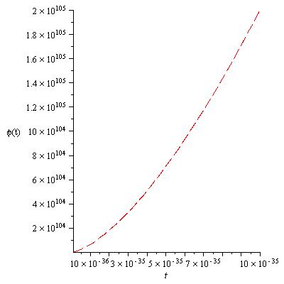
Figure 1: The shape of Scalar field is the same for $0<n<1$, the value of the constant $M_{-1}$ tells us how the scalar field grows, curve reaches the highest and lowest altitude for large and small values of the constant $M_{-1}$ respectively. In this case $n=0.8$ and $M_{-1}=10^{75}$

This solution was found with $\beta=1$, so in this case the physical quantities take a form

$$\rm-P=\rho=C_{1}M_{-1}t^{\frac{(1-a)}{2}}[I_{\nu}(\sqrt{c}t)].$$ (28)

Case II
Radiation $\rm(\gamma=\frac{1}{3})$. In this case the equation (24) is written as

$$\rm 2\frac{\ddot{A}}{A}+4\left(\frac{\dot{A}}{A}\right)^{2}+5\frac{\dot{A}}{A}\frac{\dot{\phi}}{\phi}+\frac{\ddot{\phi}}{\phi}-\frac{16}{3}\pi\frac{\rho}{\phi}=0,$$ (29)

now (23) and $\frac{\rho}{\phi}$ into (29), after some algebra we have

$$\rm t^{2}\ddot{\phi}+\frac{5}{n}t\dot{\phi}+\left[\frac{6-2n}{n^{2}}\right]\phi=\frac{16}{3}\pi\frac{M_{1/3}}{(nD)^{4/n}}t^{2-\frac{4}{n}},$$

$$\rm t^{2}\ddot{\phi}+at\dot{\phi}+b\phi=dt^{m},$$ (30)

where $\rm a=\frac{5}{n}$, $\rm b=\frac{6-2n}{n^{2}}$, $\rm d=\frac{16\pi}{3}\frac{M_{1/3}}{[nD]^{4/n}}$, and $\rm m=\frac{2n-4}{n}$.
We need to solve the equation (30), so taking account the following transformation $\rm t=e^{x}$, then (30) is rewritten as

$$\rm\frac{d^{2}\phi}{dx^{2}}+a_{1}\frac{d\phi}{dx}+b\phi=de^{mx},$$ (31)

where $\rm a_{1}=a-1$, now using the next transformation

$$\rm\phi=\omega e^{-\frac{1}{2}a_{1}x}.$$ (32)

So the equation (31) is now

$$\rm\frac{d^{2}\omega}{dx^{2}}+f\omega=de^{mx+\frac{1}{2}a_{1}x},\qquad f=\left(b-\frac{1}{4}a_{1}^{2}\right).$$ (33)

The solution of equation (33) depend the sing of the constant $f$, but remembering that $0<n<1$, so $f=-\left(\frac{n-1}{2n}\right)^{2}<0$, then the solution is

$$\rm\omega=C_{1}\cosh(k_{1}x)+C_{2}\sinh(k_{1}x)$$

$$\rm+\frac{d}{k_{1}}\int_{x_{0}}^{x}e^{(m+\frac{a_{1}}{2})\xi}\sinh[k_{1}(x-\xi)]d\xi,$$ (34)

where $\rm x_{0}$ is an arbitrary number and $\rm f=-k_{1}^{2}<0$. Now solving the integral that appear in equation (34) with $\rm\sigma=m+\frac{a_{1}}{2}$, we have the solution to $\omega$ is the following

$$\rm\omega(x)=C_{1}\cosh(k_{1}x)+C_{2}\sinh(k_{1}x)+$$

$$\rm\frac{d}{k_{1}}\left[\frac{k_{1}}{\sigma^{2}-k_{1}^{2}}e^{\sigma x}+\frac{e^{(\sigma+k_{1})x_{0}}}{2(k_{1}+\sigma)}e^{-k_{1}x}+\frac{e^{-(k_{1}-\sigma)x_{0}}}{2(k_{1}-\sigma)}e^{k_{1}x}\right].$$ (35)

Finally using the transformation $\rm t=e^{x}$, with $\rm x=\ln|t|$, then the equation (32) became

$$\rm\phi(t)=C_{1}\cosh(k_{1}\ln|t|)t^{-\frac{1}{2}a_{1}}+C_{2}\sinh(k_{1}\ln|t|)t^{-\frac{1}{2}a_{1}}$$

$$\rm+\frac{d}{k_{1}}\left[\frac{k_{1}}{\sigma^{2}-k_{1}^{2}}t^{\sigma-\frac{1}{2}a_{1}}+\frac{e^{(\sigma+k_{1})x_{0}}}{2(k_{1}+\sigma)}t^{-(k_{1}+\frac{1}{2}a_{1})}\right]$$

$$\rm+\frac{d}{k_{1}}\left[\frac{e^{-(k_{1}-\sigma)x_{0}}}{2(k_{1}-\sigma)}t^{k_{1}-\frac{1}{2}a_{1}}\right].$$ (36)

Equation (36) represent the solution to scalar field in the Radiation time and depend of the constants that appear there. Where $a_{1}=\frac{5-n}{n}$, $\sigma=\frac{3}{2}-\frac{3}{2n}$, $d=\frac{16}{3}\pi\frac{M_{1/3}}{(nD)^{4/n}}$, $k_{1}=\frac{1-n}{2n}$, note that all constants depend on $n$ and $0<n<1$.

Figure (2) shows the shape of the scalar field $\phi$ in the inflation and radiation epoch, in the inflation time $\phi$ is growing, but in the transition between inflation and radiation epoch, the scalar field slows its expansion and then decrease in the radiation time, perhaps due to the presence of the first particles. In the transition we must consider that the constant $M_{\gamma}$ must change for each stage of the universe.

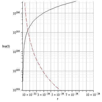
Figure 2: $\rm Log(\phi)vs\,t$. The scalar field is increasing in the inflation epoch, but in the radiation time the scalar field decrease.

Case III
Stiff matter ($\gamma=1$), then the equation (24) is written as

$$2\frac{\ddot{A}}{A}+4\left(\frac{\dot{A}}{A}\right)^{2}+5\frac{\dot{A}}{A}\frac{\dot{\phi}}{\phi}+\frac{\ddot{\phi}}{\phi}=0,$$ (37)

substituting equation (23) in (37), yielding

$$\rm t^{2}\ddot{\phi}+\frac{5}{n}t\dot{\phi}+\left[\frac{6-2n}{n^{2}}\right]\phi=0,$$

$$\rm t^{2}\ddot{\phi}+at\dot{\phi}+b\phi=0,$$ (38)

with $a=\frac{5}{n}$, $b=\frac{6-2n}{n^{2}}$, with the following solution

$$\phi(t)=|t|^{\frac{1-a}{2}}(c_{1}|t|^{\mu}+c_{2}|t|^{-\mu}),\qquad(1-a)^{2}>4b,$$ (39)

where $c_{1}$, $c_{2}$ are constants and $\mu=\frac{n-1}{2n}$.

Then the solution to equation (38) is

$$\rm\phi(t)=c_{1}|t|^{1-\frac{3}{n}}+c_{2}|t|^{-\frac{2}{n}}.$$ (40)

Figure (3) shows that the contribution of the scalar field at the beginning was significantly, but decreasing exponentially along the time, also we note that $\phi$ decreases more quickly than in the radiation time.

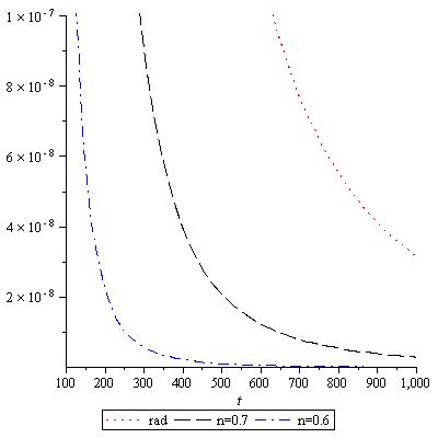
Figure 3: The black and blue line represents the behavior of the scalar field in the stiff matter epoch. The red line represents the solution to the radiation epoch obtained in the previous section, we note that in the transition between radiation and stiff matter, the scalar field decreases more quickly than predicted radiation curve. For very large times $\phi\rightarrow 0$.

Finally, the physical quantities take the form:

$$\rm P=\rho=M_{1}(Dnt)^{\frac{-6}{n}}(c_{1}t^{1-\frac{3}{n}}+c_{2}t^{-\frac{2}{n}})^{\beta}.$$ (41)

where $\beta=\frac{\lambda_{0}(3+2\omega)}{2}-1$.

On the other hand, remembering that our results are based on the Berman’s law Berman , we obtain an expression for the average scalar factor (equations 22-23), taking the equation (23)(case $n\neq 0$) to solve the corresponding set of equations. Figure (4) shows the behavior of scalar factor to different values of $n$ ($0<n<1$). Note that when $n$ increases, the scalar factor grows rapidly, i.e. the slope of the curve is large, but for certain values of $n$, the slope of the curve approaches a plane curve. Remembering $D$ is a constant and in this case has the role of slope of the curve. With the observational data in your epoch, Berman Berman calculated this value for dust matter, yielding to the value $D\cong 5.0\times 10^{28}\frac{cm^{2}}{s}$. Considering the shape of the scale factor for some values in the n parameter, we say that the expansion scenary today corresponds for a special value to n, in the branch $\rm[0.3,1)$ figure (4(b)). These intervals can be modified when one calculate the value to the constant D considering the observational data today. This calculation will be part of forthcoming paper.

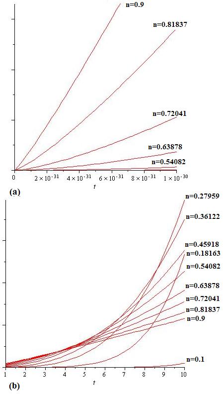
Figure 4: (a) Behavior of the scalar factor in the inflation and radiation time, we note that for $0.6<n<1$ is when the universe has a rapid expansion. (b) after radiation time the shape of the scalar field is modified so the expansion scenary today correspond to $0.3<n<1$. $D$ is the slope of the curve, but this constant have different values for each age of the universe. Berman Berman calculate this value for dust matter ($\gamma=0$) with $D\cong 5.0\times 10^{28}\frac{cm^{2}}{s}$.

IV Lagrangian and Hamiltonian densities in SCC

In the previous section using the Berman’s law, were solved the Einstein field equations. Now we will use the classical approach to find solutions to $(\rho,A,\phi)$. The corresponding Lagrangian density using (8) into (1)

$$\rm{\cal L}=6\frac{A\phi{\dot{A}}^{2}}{N}+6\frac{A^{2}\dot{A}\dot{\phi}}{N}-\frac{\omega A^{3}{\dot{\phi}}^{2}}{N\phi}+16\pi A^{3}\rho N,$$ (42)

the momenta are $(\Pi_{q}=\frac{\partial\cal L}{\partial\dot{q}})$

$$\rm\Pi_{A}=\rm 12\frac{A\phi\dot{A}}{N}+6\frac{A^{2}\dot{\phi}}{N},\qquad\Pi_{\phi}=\rm 6\frac{A^{2}\dot{A}}{N}-2\frac{\omega A^{3}\dot{\phi}}{N\phi},$$

$$\rm\dot{A}=\frac{N}{6(3+2\omega)\phi A^{2}}\left(3\phi\Pi_{\phi}+\omega A\Pi_{A}\right),$$ (43)

$$\rm\dot{\phi}=\frac{N}{2(3+2\omega)A^{3}}\left(A\Pi_{A}-2\phi\Pi_{\phi}\right),$$ (44)

when we write the canonical Lagrangian density $\rm{\cal L}_{canonical}=\Pi_{q}\dot{q}-N{\cal H}$, we obtain the corresponding Hamiltonian density as

$$\rm{\cal H}=\frac{A^{-3}}{12a_{0}\phi}[-6\phi^{2}\Pi_{\phi}^{2}+\omega A^{2}\Pi_{A}^{2}+6A\phi\Pi_{A}\Pi_{\phi}$$

$$-192\pi a_{0}A^{6}\phi\rho],\qquad a_{0}=(3+2\omega),\qquad$$ (45)

IV.1 Classical scheme: Hamilton-Jacobi equation

Using the gauge $\rm N=12a_{0}\phi A^{3}$, and the transformation in the momenta $\rm\Pi_{q}=\frac{\partial S}{\partial q}$, where S is known as the superpotential function, with this, the Hamiltonian density is written as (we include the equation (17) in this last equation)

$$\rm-6\phi^{2}\left(\frac{\partial S}{\partial\phi}\right)^{2}+\omega A^{2}\left(\frac{\partial S}{\partial A}\right)^{2}+6A\phi\left(\frac{\partial S}{\partial A}\right)\left(\frac{\partial S}{\partial\phi}\right)$$

$$\rm-192\pi a_{0}M_{\gamma}A^{-3(\gamma-1)}\phi^{(\beta+1)}=0,$$ (46)

This is the differential equation in the Hamilton-Jacobi theory, equation (46), which can be solved for general barotropic fluid using the method of Lagrange-Charpit Elsgoltz ; delgado ; lopez , solutions that will be presented elsewhere. So in the follow, for simplicity we shall use the stiff matter case, $\gamma=1$ (so $\beta+1=\frac{\lambda_{0}(3+2\omega)}{2}$). Using $\rm S(A,\phi)=S_{1}(A)+S_{2}(\phi)$, we have

$$\rm-6\phi^{2}\left(\frac{dS_{2}}{d\phi}\right)^{2}+\omega A^{2}\left(\frac{dS_{1}}{dA}\right)^{2}+6A\phi\left(\frac{dS_{1}}{dA}\right)\left(\frac{dS_{2}}{d\phi}\right)$$

$$\rm-192\pi a_{0}M_{1}\phi^{(\beta+1)}=0,$$ (47)

identifiying $\rm A\frac{dS_{1}}{dA}=c_{1}=constant$, then (47) can be solve as

$$\rm\frac{dS_{2}}{d\phi}=\frac{c_{1}}{2\phi}\mp\frac{1}{6\phi}\sqrt{3c_{1}^{2}a_{0}-1152\pi a_{0}M_{1}\phi^{(\beta+1)}},$$ (48)

using (43) and (44) we find that $c_{1}a_{0}=\frac{\dot{A}}{A}+\frac{1}{2}\frac{\dot{\phi}}{\phi}$, then (48) can be determined as

$$\rm\phi(t)=\phi_{0}\,sech^{\frac{2}{\beta+1}}\left(-c_{0}\sqrt{3a_{0}}t\right),$$ (49)

so, the solution for the scale factor A, become

$$\rm A(t)=A_{0}\cosh^{\frac{1}{\beta+1}}\left(-c_{0}\sqrt{3a_{0}}t\right)\exp\left[\frac{c_{0}a_{0}t}{\beta+1}\right].$$ (50)

V Conclusions

In this paper we have investigated FRW cosmological model of the universe in the framework of Barber’s second self-creation theory, we obtain a solution for three cases: inflation ($\gamma=-1$), radiation ($\gamma=\frac{1}{3}$) and stiff matter ($\gamma=1$), in the first case the scalar field was an increasing function and depends on the constant $M_{-1}$, we note that in the transition between inflation and radiation epoch, the scalar field stop its expansion and then decreases. This behavior is due to the constant $M_{\gamma}$ that appear in the solution must change for each stage of the universe and we must also consider the presence of the first particles in the radiation time, in the stiff matter time the scalar field decrease exponentially and for very long time $\phi\rightarrow 0$. Such that currently, the scalar field contribution is very small.
In addition we found a new parameter $\lambda_{0}\neq\lambda=\frac{2}{3+2\omega}$ more general than barber’s parameter, but when $\lambda_{0}=\lambda$ the solution of density (17) is the same that in general relativity, so there is no contribution of the scalar field. Our results are preliminary with this and will depend on how to adjust the constant with current observations. On the other hand, the classical solution found under the Hamilton-Jacobi approach (stiff matter) have an structure more general. Moreover, the feeling is that in some approximation, this class of solution could be tied with the Berman’s law.

- (1) M. S. Berman and F. M. Gomide, Nuovo Cim. 74B, 182 (1983).
- (2) S. Weinberg, Gravitation and Cosmology: Principles and Aplications of the General Theory of Relativity, John Wiley and Sons, Inc. New York London Sydney Toronto, (1972).
- (3) G. A. Barber, Gen. Rel. And Grav. 14, 117 (1982).
- (4) G. A. Barber, A New Self-Creation Cosmology A semi-metric theory of gravitation Astrophysics and Space Science 282, 683-730 (2002).
- (5) G. A. Barber, Self-Creation Cosmology ArXiv:1009.5862v2 (2010).
- (6) C. P. Singh, and S. Kumar, Int. J. Mod. Phys. D 15, 419 (2006).
- (7) C. P. Singh and, S. Kumar, Astrophys Space Sci Bianchi type-II space-times with constant deceleration parameter in self creation cosmology 310, 31 (2007).
- (8) C. P. Singh, S. Ram, and M. Zeyauddin, Astrophys. Space Sci. 315, 181 (2008).
- (9) M. K. Singh, M. K. Verma, and Shri Ram, Adv. Studies Theor. Phys. 6, 117-127 (2012).
- (10) T. Singh, Astrophys. Space Sci. 102, 67 (1984).
- (11) L. O. Pimentel, Astrophys. Space Sci. 116, 395 (1985).
- (12) H. H. Soleng, Astrophys. Space Sci. 138, 19 (1987a).
- (13) H. H. Soleng, Astrophys. Space Sci. 139, 13 (1987b).
- (14) D.R.K. Reddy, Astrophys. Space Sci. 133, 189 (1987).
- (15) R. Venkateswarlu, D.R.K. Reddy, Astrophys. Space Sci. 168, 193 (1990).
- (16) R. Shri, C. P. Singh, Astrophys. Space Sci. 257, 123 (1998a).
- (17) R. Shri, C. P. Singh, Astrophys. Space Sci. 257, 287 (1998b).
- (18) G. Mohanty, B. Mishra, and R. Das, Bull. Inst. Math. Acad. Sin. (ROC) 28, 43 (2000).
- (19) A. Pradhan, A. K. Vishwakarma, Int. J. Mod. Phys. D 11, 1195 (2002a).
- (20) A. Pradhan, A. K. Vishwakarma, Indian J. Pure Appl. Math. 33, 1239 (2002b).
- (21) R. C. Sahu, U. K. Panigrahi, Astrophys. Space Sci. 288, 601 (2003).
- (22) R. Venkateswarlu, P. K. Kumar, Astrophys. Space Sci. 301, 73 (2006).
- (23) V. R. Chirde, P. N. Rahate, Int J Theor Phys. 51, 2262-2271 (2012).
- (24) D. S. Chouan and A. Pradhan, Some exact Bianchi type-V Cosmological models in Saenz Ballester theory of gravitation
- (25) Andrei D. Polyanin and Valentin F. Zaitesev, Exact Solutions for Ordinary Differential Equations, Chapman and Hall/CRC, (2003).
- (26) L. Elsgoltz, Ecuaciones Diferenciales y cálculo variacional, Edit. Mir Moscu, (1969).
- (27) M. Delgado, SIAM Rev. 39, 298 (1997). The Lagrange-Charpit method.
- (28) G. López, Partial Differential equations of first order and their applications to physics, World Scientific Pub. (1999).