A Transport for imaging process

Abstract

This work originates from a heart’s images tracking which is to generate an apparent continuous motion, observable through intensity variation from one starting image to an ending one both supposed segmented. Given two images $\rho_{0}$ and $\rho_{1}$, we calculate an evolution process $\rho(t,\cdot)$ which transports $\rho_{0}$ to $\rho_{1}$ by using the optical flow. In this paper we propose an algorithm based on a fixed point formulation and a space-time least squares formulation of the transport equation for computing a transport problem. Existence results are given for a transport problem with a minimum divergence for a dual norm or a weighted $H^{1}_{0}$-semi norm, for the velocity. The proposed transport is compare with the transport introduced by Dacorogna-Moser. The strategy is implemented in a 2D case and numerical results are presented with a first order Lagrange finite element, showing the efficiency of the proposed strategy.

keywords AMS Classification 35F40; 35L85; 35R05;

1 Introduction

Modern medical imaging modalities can provide a great amount of information to study the human anatomy and physiological functions in both space and time. In cardiac magnetic resonance imaging (MRI) for example, several slices can be acquired to cover the heart in 3D and at a collection of discrete time samples over the cardiac cycle. From these partial observations, the challenge is to extract the heart’s dynamics from these input spatio-temporal data throughout the cardiac cycle [14], [16].

Image registration consists in estimating a transformation which insures the warping of one reference image onto another target image (supposed to present some similarity). Continuous transformations are privileged, the sequence of transformations during the estimation process is usually not much considered. Most important is the final resulting transformation and not the way one image will be transformed to the other. Here, we consider a reasonable interpolation process to continuously map the image intensity functions between two images in the context of cardiac motion estimation and modeling.

The aim of this paper is to present, in the context of optical flow, an algorithm to compute a time dependent transportation plan without using lagrangian techniques.

The paper is organized as follows. The introduction is ended, by recalling the optical flow model (OF) . In section 2, the algorithm is presented, and its convergence is discussed. In section 3 it is shown that the solutions obtained with the proposed algorithm are the solutions minimizing the same energy than the time dependent optimal mass transportation problem. Section 4 is devoted to numerical results. In particular a 2D cardiac medical image is considered.

1.1 The optical flow (OF) method

Let $\rho$ be the intensity function, and $v$ be the velocity of the apparent motion of brightness pattern. An image sequence is considered via the gray-value map $\rho:Q=(0,1)\times\Omega\rightarrow\mathbb{R}$ where $\Omega\subset\mathbb{R}^{d}$ is a bounded regular domain, the support of images, for $d=1,2,3$. If image points move according to the velocity field $v:\,Q\rightarrow\mathbb{R}^{d}$, then gray values $\rho(t,X(t,x))$ are constant along motion trajectories $X(t,x)$. One obtains the optical flow equation.

$$\frac{d}{dt}\rho(t,X(t,x))=\partial_{t}\rho(t,X(t,x))+\left(\,{v}\,|\,{\nabla_{X}\rho(t,X(t,x))}\,\right)_{\mathbb{R}^{d}}=0.$$ (1)

The previous equations lead to an ill-posed problem for the unknown $(\rho,v)$. Variational formulations or relaxed minimizing problems for computing jointly $(\rho,v)$ have been first proposed in [4] and after by many other authors. Here our concern is somewhat different. Finding $(\rho,v)$ simultaneously is possible by solving a mass transport problem. Similarly to the work developed in [5, 6], a characterization of $(\rho,v)$ as solution of a minimizing problem is developed.

Let $\rho_{0}$ and $\rho_{1}$ be the cardiac images between two times arbitrary fixed to zero and one, the mathematical problem reads: find $\rho$ the gray level function defined from $Q$ with values in $[0,1]$ verifying

$$\left\{\begin{array}[]{l}\partial_{t}\rho(t,x)+\left(\,{(v(t,x)}\,|\,{\nabla\rho(t,x)}\,\right)=0,\,(t,x)\in(0,1)\times\Omega\\ \rho(0,x)=\rho_{0}(x);\quad\rho(1,x)=\rho_{1}(x)\,x\in\Omega\end{array}\right.$$ (2)

The velocity function $v$, is determined in order to minimize the functional.

$$\inf_{\rho,v}\int_{0}^{1}\int_{\Omega}\rho(t,x)\|v(t,x)\|^{2}\,dtdx.$$ (3)

Thus we get an image sequence through the gray-value map $\rho$. Let us mention [3], for example, where the optimal mass transportation approach is used in images processing. In this work, the optimal transport problem in 2D is decomposed in several 1D optimal transport problems which are easier to numerically solved. The algorithm proposed here, is based on a least squares formulation for the transport equation ([9] for example), which differs from the methods proposed in [3], or in [5]. Notice that the proposed transport in this paper differs from the optimal transportation, studied e.g. in the book of C. Villani [20].

2 Algorithm for solving the optical flow

In this section, an algorithm is presented to solve the optical flow given by equations (2), and (3). Let us first specify our hypotheses.

• The domain $\Omega$ is a bounded $C^{2,\alpha}$ domain satisfying the exterior sphere condition.

• The functions $\rho_{i}\in C^{1,\alpha}(\overline{\Omega})$ for $i=0,1$, with $\rho_{0}=\rho_{1}\text{ on }\partial\Omega$. Moreover there exist two constants such that $0<\underline{\beta}\leq\rho_{i}\leq\overline{\beta}$ in $\Omega$.

Let $\rho^{0}\in C^{1,\alpha}([0,1]\times\overline{\Omega})$ be given by $\rho^{0}(t,x)=(1-t)\rho_{0}(x)+t\rho_{1}(x)$. We have $\|\partial_{t}\rho^{0}\|_{C^{0,\alpha}([0,1]\times\overline{\Omega})}\leq C(\rho_{0},\rho_{1})$ and $\partial_{t}\rho^{0}|_{\partial\Omega}=0$.

For each $t\in[0,1]$, our need to solve problem (2)-(3) is a velocity field vanishing on $\partial\Omega$. To do so, the following method is used.

Assume that $\rho^{n}\in C^{1,\alpha}([0,1]\times\overline{\Omega})$ is given with $\rho^{n}(0,x)=\rho_{0}(x)$, and $\rho^{n}(1,x)=\rho_{1}(x)$ for all $x\in\Omega$.

• Compute $\eta^{n+1}$ such that

  $$\left\{\begin{array}[]{l}-\mathop{\rm div}\nolimits(\rho^{n}(t,\cdot)\nabla\eta^{n+1})=0\,\text{ in }\Omega\\ \displaystyle\rho^{n}(t,\cdot)\frac{\partial{\eta^{n+1}}}{\partial{n}}=1\quad\text{ on }\partial\Omega,\end{array}\right.$$ (4)

  and set $\displaystyle C^{n+1}(t)=\frac{1}{|\partial\Omega|}\int_{\Omega}\partial_{t}\rho^{n}\eta^{n+1}\,dx$.

• For each $t\in[0,1]$ compute $\varphi^{n+1}$ solution of

  $$\left\{\begin{array}[]{l}-\mathop{\rm div}\nolimits(\rho^{n}(t,\cdot)\nabla\varphi^{n+1})=\partial_{t}\rho^{n}(t,\cdot),\,\text{ in }\Omega\\ \varphi^{n+1}=C^{n+1}(t)\quad\text{ on }\partial\Omega.\end{array}\right.$$ (5)

• Set $v^{n+1}=\nabla\varphi^{n+1}$.

• Compute $\rho^{n+1}$, $L^{2}$-least squares solution of

  $$\left\{\begin{array}[]{l}\partial_{t}\rho^{n+1}(t,x)+\left(\,{v^{n+1}(t,x)}\,|\,{\nabla\rho^{n+1}(t,x)}\,\right)=0,\;(t,x)\in(0,1)\times\Omega,\\ \rho^{n+1}(0,x)=\rho_{0}(x);\quad\rho^{n+1}(1,x)=\rho_{1}(x)\;x\in\Omega.\end{array}\right.$$ (6)

Remark 2.1

If the requirement $\rho_{0}{\big{|}_{\partial\Omega}}=\rho_{1}{\big{|}_{\partial\Omega}}$ is canceled in hypothesis H2, then the boundary condition of problem (5) is replaced by $\displaystyle\frac{\partial{\varphi^{n+1}}}{\partial{n}}=0$ and we do not need anymore the constants $C^{n+1}$.

For each $t\in[0,1]$, since $\rho^{n}(t,\cdot)$, and $\partial_{t}\rho^{n}(t,\cdot)\in C^{0,\alpha}(\overline{\Omega})$, theorem 6.14 p. 107 of [13] applies, and there exists a unique $\varphi^{n+1}(t,\cdot)\in C^{2,\alpha}(\overline{\Omega})$ solution of problem (5). In problem (5) the time $t$ is a parameter. Since $\rho^{n}\in C^{1,\alpha}$, and $\partial_{t}\rho^{n}\in C^{0,\alpha}$, and $C^{n+1}\in C^{0,\alpha}$, the classical $C^{2,\alpha}(\overline{\Omega})$ a priori estimates for solutions to elliptic problems allow us to show that $\varphi^{n+1}$ is a $C^{0,\alpha}$ function with respect to time. So we have

$$\|\varphi^{n+1}\|_{C^{0,\alpha}([0,1];C^{2,\alpha}(\overline{\Omega}))}\leq M(\|C^{n}\|_{C^{0,\alpha}([0,1])}+\|\partial_{t}\rho^{n}\|_{C^{0,\alpha}([0,1]\times\overline{\Omega})}).$$

Consider the extension of $\varphi^{n+1}$ by $C^{n+1}$ outside of the domain $\Omega$, still denoted by$\varphi^{n+1}$. Since the right hand side of equation (5) vanishes on $\partial\Omega$, this extension is regular, so the function $v^{n+1}$ vanish outside $\Omega$ and belongs to $C^{0,\alpha}([0,1];C^{1,\alpha}(\mathbb{R}^{2}))$.

Define the flow $X^{n+1}_{+}(s,t,x)\in C^{1,\alpha}([0,1]\times[0,1]\times\mathbb{R}^{2};\mathbb{R}^{2})$ by

$$\left\{\begin{array}[]{l}\displaystyle\frac{d}{ds}X^{n+1}_{+}(s,t,x)=+v^{n+1}(s,X^{n+1}_{+}(s,t,x))\,\text{ in }(0,1)\\ X^{n+1}_{+}(t,t,x)=x.\\ \end{array}\right.$$ (7)

This flows will be constant for $x\in\partial\Omega$. Observe that solving the transport equation (6) in the least-squares sense is equivalent to solve this equation on each integral curves defined by (7).

Set $r(s)=\rho^{n+1}(s,X^{n+1}_{+}(s,t,x))$, and express equation (6) along the integral curves of equation (7). The equation is reduced to the following ordinary differential equation with initial and final conditions.

$$\left\{\begin{array}[]{l}\displaystyle\frac{d}{ds}r(s)=0\\ r(0)=\rho_{0}(X^{n+1}_{+}(0,t,x));\,r(1)=\rho_{1}(X^{n+1}_{+}(1,t,x)).\\ \end{array}\right.$$ (8)

The $L^{2}$ least squares solution of (8) minimizes $\displaystyle\frac{d}{ds}r(s)$, and is given by:

$$r(s)=(1-s)\rho_{0}(X^{n+1}_{+}(0,t,x))+s\rho_{1}(X^{n+1}_{+}(1,t,x)).$$

Therefore the following representation formula for the function $\rho^{n+1}$ is proved.

Lemma 2.2

The $L^{2}$-least squares solution of problem (6) is given by

$$\begin{array}[]{c}\rho^{n+1}(t,x)=(1-t){\rho_{0}(X^{n+1}_{+}(0,t,x))}+t{\rho_{1}(X^{n+1}_{+}(1,t,x))}.\end{array}$$ (9)

Remark that the regularity of the function $\rho^{n+1}$ is a consequence of the regularity of the flow $X_{+}^{n+1}$.

Let us now consider the convergence of the algorithm (4)-(6).

Theorem 2.3

There exist $(\rho,\varphi)\in C^{1}([0,1]\times\overline{\Omega};\mathbb{R}_{+}^{*})\times C^{0}([0,1];C^{2}(\overline{\Omega}))$, $L^{2}$-least squares solution, respectively solution of

$$\left\{\begin{array}[]{l}\partial_{t}\rho+\left(\,{\nabla\varphi}\,|\,{\nabla\rho}\,\right)=0,\quad\mathrm{in}\,(0,1)\times\Omega\\ \rho(0,x)=\rho_{0}(x);\quad\rho(1,x)=\rho_{1}(x)\quad\mathrm{in}\,\Omega\\ \end{array}\right.$$ (10)

$$\left\{\begin{array}[]{l}-\mathop{\rm div}\nolimits(\rho(t,\cdot)\nabla\varphi)=\partial_{t}\rho(t,\cdot),\quad\mathrm{in}\,\Omega\\ \varphi=C(t)\quad\mathrm{and}\quad\nabla\varphi=0\quad\mathrm{on}\,\partial\Omega\\ \end{array}\right.$$ (11)

with $C(t)$ defined as follow.

$$\left\{\begin{array}[]{l}-\mathop{\rm div}\nolimits(\rho(t,\cdot)\nabla\eta)=0\;\mathrm{in}\,\Omega\\ \rho(t,\cdot)\,\partial_{n}\eta=1\;\mathrm{on}\,\partial\Omega\\ C=\displaystyle\frac{1}{|\partial\Omega|}\int_{\Omega}\partial_{t}\rho\,\eta\,dx.\end{array}\right.$$ (12)

Proof. Since $\|v^{0}\|_{C^{0,\alpha}([0,1])}+\|\partial_{t}\rho^{0}\|_{C^{0,\alpha}([0,1]\times\overline{\Omega})}$ is bounded, $\|\varphi^{n+1}\|_{C^{0,\alpha}([0,1];C^{2,\alpha}(\overline{\Omega}))}$ and $\|v^{n+1}\|_{C^{0,\alpha}([0,1];C^{1,\alpha}(\mathbb{R}^{2}))}$ are uniformly bounded in $n$.

From lemma 2.2 there exists a unique $\rho^{n+1}$, the $L^{2}$-least squares solution of (6). Let us give an estimate for $D_{3}X_{+}^{n+1}$. Starting from

$$D_{1}X^{n+1}_{+}(s,t,x))=v^{n+1}(s,X^{n+1}_{+}(s,t,x)),$$

we deduce (see [1])

$$\left\{\begin{array}[]{l}D_{3}D_{1}X^{n+1}_{+}(s,t,x)=D_{2}v^{n+1}(s,X^{n+1}_{+}(s,t,x))D_{3}X^{n+1}_{+}(s,t,x)\\ D_{3}X^{n+1}_{+}(t,t,x)=Id.\\ \end{array}\right.$$ (13)

Since $D_{3}D_{1}X^{n+1}_{+}(s,t,x)=D_{1}D_{3}X^{n+1}_{+}(s,t,x)$ we get

$$D_{3}X^{n+1}_{+}(s,t,x)=e^{-\int_{t}^{s}D_{2}(v^{n+1}(\tau,X^{n+1}_{+}(\tau,t,x)))\,d\tau}Id.$$ (14)

Thus $\|D_{3}v_{+}^{n+1}\|_{C^{0,\alpha}([0,1]^{2}\times\mathbb{R}^{2})}$ is uniformly bounded in $n$. Moreover we have [1]

$$D_{2}X^{n+1}_{+}(s,t,x)=\left(\,{v^{n+1}(s,t,x)}\,|\,{D_{3}X^{n+1}_{+}(s,t,x)}\,\right)$$

so $\|D_{2}v^{n+1}\|_{C^{0,\alpha}([0,1]^{2}\times\mathbb{R}2)}$ is bounded independently of $n$.

From theorem 2.2 we deduce that $\|\rho^{n+1}\|_{C^{1,\alpha}([0,1]\times\overline{\Omega})}$ is uniformly bounded. Since the embeddings

$$C^{0,\alpha}([0,1];C^{2,\alpha}(\overline{\Omega}))\hookrightarrow C^{0}([0,1];C^{2}(\overline{\Omega}))\,\mathrm{and}\,C^{1,\alpha}([0,1]\times\overline{\Omega})\hookrightarrow C^{1}([0,1]\times\overline{\Omega})$$

are relatively compact there is a subsequence of $(\rho^{n},\varphi^{n})$ solution of (4)-(6), still denoted by $(\rho^{n},\varphi^{n})$ converging to $(\rho,\varphi)$ in $C^{1}([0,1]\times\overline{\Omega})\times C^{0}([0,1];C^{2}(\overline{\Omega}))$, and $(\rho,\varphi)$ is the solution of (10)-(12) provided the boundary conditions to be justified. The condition $\nabla\varphi^{n}|_{\partial\Omega}=0$ is valid for the approximations $\varphi^{n}$ (since the functions can be extended by $C^{n}$ outside of $\Omega$). So the convergence in $C^{0}([0,1];C^{2}(\overline{\Omega}))$ yields the condition for the gradient of limit function. For the approximations of function $\rho$, the formula given in lemma 2.2 combined with the regularity result show that the boundary conditions are exactly satisfied. These conditions are thus valid for the limit function due to the convergence in $C^{1}$. $\square$ We will show in the next section that the solution minimizes the same energy as for the time dependent optimal transportation mass.

3 Interpretation of solutions to problem (10)-(12)

In this section it is shown that the solution to problem (10)-(12) is a solution to a time dependent mass transportation problem.

Zero is a bound from below of the following functional $\frac{1}{4}\int_{0}^{1}\|\partial_{t}u+\mathop{\rm div}\nolimits(u\nabla(\psi-C))\|_{L^{2}(\Omega)}^{2}\,dt$ to be minimized with respect to $(u,\psi)$.

$$0=\frac{1}{4}\int_{0}^{1}\|\partial_{t}\rho+\mathop{\rm div}\nolimits(\rho\nabla(\varphi-C))\|_{L^{2}(\Omega)}^{2}\,dt$$

thus $(\rho,\varphi-C)$ solution of (10)-(12) minimizes

$$\underset{\begin{array}[]{c}\scriptstyle\{\psi\in L^{2}((0,1);H^{1}_{0}(\Omega)),\;u\in L^{2}((0,1);L^{2}(\Omega))\\ \scriptstyle\partial_{t}u+\left(\,{u}\,|\,{\nabla\psi}\,\right)=0\\ \scriptstyle u(0)=\rho_{0};\;u(1)=\rho_{1}\text{ in }\Omega\}\end{array}}{\rm Min}\frac{1}{4}\int_{0}^{1}\|\partial_{t}u+\mathop{\rm div}\nolimits(u\nabla\psi)\|_{L^{2}(\Omega)}^{2}\,dt.$$

So the solution $(\rho,\varphi)$ of problem (10)-(12), satisfies

$$(\rho,\varphi-C)=\underset{\begin{array}[]{c}\scriptstyle\{\psi\in L^{2}((0,1);H^{1}_{0}(\Omega)),\\ \scriptstyle u\in L^{2}((0,1);L^{2}(\Omega)),\\ \scriptstyle\partial_{t}u+\left(\,{u}\,|\,{\nabla\psi}\,\right)=0,\\ \scriptstyle u(0)=\rho_{0};\;u(1)=\rho_{1}\text{ in }\Omega\}\end{array}}{\text{Argmin}}\frac{1}{4}\int_{0}^{1}\|\partial_{t}u+\mathop{\rm div}\nolimits(u\nabla\psi)\|_{H^{-1}}\,dt.$$ (15)

Theorem 3.1

Let $(\rho,\varphi)$ be the solution of problem (10)-(12) given in theorem 2.3, then it satisfies

$$(\rho,\nabla\varphi)=\underset{\begin{array}[]{c}\scriptstyle\{v\in L^{2}((0,1);\left(H^{1}(\Omega)\right)^{2}),\\ \scriptstyle u\in L^{2}((0,1);L^{2}(\Omega)),\\ \scriptstyle\partial_{t}u+\mathop{\rm div}\nolimits(uv)=0,\\ \scriptstyle\partial_{t}u+\left(\,{v}\,|\,{\nabla u}\,\right)=0,\\ \scriptstyle u(0)=\rho_{0};\,u(1)=\rho_{1}\text{ in }\Omega\}\end{array}}{\rm Argmin}\int_{0}^{1}\int_{\Omega}u\|v\|^{2}\,dxdt.\\$$ (16)

Proof. Observe that in problem (16), the transport equation is solved with a $L^{2}$-least square procedure. This is equivalent to find $\xi=u-(1-t)\rho_{0}+t\rho_{1}$ such that

$$\partial_{t}\xi+\left(\,{v}\,|\,{\nabla\xi}\,\right)=P_{R}(\rho_{1}-\rho_{0}+\left(\,{v}\,|\,{\nabla\left((1-t)\rho_{0}+t\rho_{1}\right)}\,\right)$$

where $P_{R}$ is the $L^{2}$ projection onto the range of the transport operator for the velocity $v$.

For $u\in L^{\infty}(\Omega)$, the expression $v\mapsto\mathop{\rm div}\nolimits(uv)$ is well defined as a linear continuous on $H^{1}_{0}(\Omega)$. If moreover $0<\underline{\beta}\leq u\leq\overline{\beta}$ in $\Omega$, let $H=H^{1}_{0}(\Omega)$ be equipped with the following inner product.

$$(\theta,\psi)=\int_{\Omega}u\left(\,{\nabla\theta}\,|\,{\nabla\psi}\,\right)\,dx,$$

which induces a semi-norm which is equivalent to the $H^{1}$-norm. The Riesz theorem claims that for the linear continuous form

$$\mathcal{L}_{v}(\psi)=<-\mathop{\rm div}\nolimits{(uv)},\psi>_{H;H^{\prime}},$$

there is a unique $\theta\in H$ such that

$$\mathcal{L}_{v}(\psi)=\int_{\Omega}u\left(\,{\nabla\theta}\,|\,{\nabla\psi}\,\right)\,dx,\,\forall\psi\in H.$$

Therefore $v=\nabla\theta$ for a $\theta\in H^{1}_{0}(\Omega)$ and problem (16) is reduced to

$$(\rho,\nabla\varphi)=\underset{\begin{array}[]{c}\scriptstyle\{\psi\in L^{2}((0,1);H^{1}_{0}(\Omega)\cap H^{2}(\Omega)),\\ \scriptstyle u\in L^{2}((0,1);L^{2}(\Omega)),\\ \scriptstyle\partial_{t}u+\mathop{\rm div}\nolimits(u\nabla\psi)=0,\\ \scriptstyle\partial_{t}u+\left(\,{\nabla\psi}\,|\,{u}\,\right)=0,\\ \scriptstyle\,u(0)=\rho_{0};\,u(1)=\rho_{1}\text{ in }\Omega\}\end{array}}{\rm Argmin}\int_{0}^{1}\int_{\Omega}u\|\nabla\psi\|^{2}\,dxdt.$$ (17)

or

$$(\rho,\nabla\varphi)=\underset{\begin{array}[]{c}\scriptstyle\{-\psi\in L^{2}((0,1);H^{1}_{0}(\Omega)\cap H^{2}(\Omega)),\\ \scriptstyle u\in L^{2}((0,1);L^{2}(\Omega)),\\ \scriptstyle\partial_{t}u-\mathop{\rm div}\nolimits(u\nabla\psi)=0,\\ \scriptstyle\partial_{t}u-\left(\,{u}\,|\,{\nabla\psi}\,\right)=0,\\ \scriptstyle u(0)=\rho_{0};\,u(1)=\rho_{1}\text{ in }\Omega\}\end{array}}{\rm Argmin}\int_{0}^{1}\int_{\Omega}u\|\nabla\psi\|^{2}\,dxdt.$$ (18)

Since

$$\int_{\Omega}u\|\nabla\psi\|^{2}\,dx=\|-\mathop{\rm div}\nolimits(u\nabla\psi)\|^{2}_{H^{-1}},$$

problem (17) reads:

$$(\rho,\nabla\varphi)=\underset{\begin{array}[]{c}\scriptstyle\{-\psi\in L^{2}((0,1);H^{1}_{0}(\Omega)\cap H^{2}(\Omega)),\\ \scriptstyle u\in L^{2}((0,1);L^{2}(\Omega)),\\ \scriptstyle\partial_{t}u-\mathop{\rm div}\nolimits(u\nabla\psi)=0,\\ \scriptstyle\partial_{t}u-\left(\,{u}\,|\,{\nabla\psi}\,\right)=0,\\ \scriptstyle u(0)=\rho_{0};\,u(1)=\rho_{1}\text{ in }\Omega\}\end{array}}{\rm Argmin}\int_{0}^{1}\|\mathop{\rm div}\nolimits(-u\nabla\psi)\|^{2}_{H^{-1}}\,dt.$$ (19)

From the definition of the linear form $\mathcal{L}$, observe that

$$\frac{1}{4}\|\mathop{\rm div}\nolimits(-u\nabla\psi)+\partial_{t}u\|^{2}_{H^{-1}}=\|\mathop{\rm div}\nolimits(-u\nabla\psi)\|^{2}_{H^{-1}},$$

so problem (19) reads:

$$(\rho,\nabla\varphi)=\underset{\begin{array}[]{c}\scriptstyle\{\psi\in L^{2}((0,1);H^{1}_{0}(\Omega)\cap H^{2}(\Omega)),\\ \scriptstyle u\in L^{2}((0,1);L^{2}(\Omega)),\\ \scriptstyle\partial_{t}u+\mathop{\rm div}\nolimits(u\nabla\psi)=0,\\ \scriptstyle\partial_{t}u+\left(\,{u}\,|\,{\nabla\psi}\,\right)=0,\\ \scriptstyle u(0)=\rho_{0};\,u(1)=\rho_{1}\text{ in }\Omega\}\end{array}}{\rm Argmin}\frac{1}{4}\int_{0}^{1}\|\mathop{\rm div}\nolimits(u\nabla\psi)+\partial_{t}u\|^{2}_{H^{-1}}\,dt.$$ (20)

Gathering (15) with the previous result proves the theorem. $\square$

Remark 3.2

The proposed transport is a one which minimizes the divergence of the velocity in a weighted dual norm of $H^{1}_{0}$

Remark 3.3

The Dacorogna-Moser transport [10] $\rho(t,x)=(1-t)\rho_{0}(x)+t\rho_{1}(x)$ with

$$\left\{\begin{array}[]{l}-\Delta\varphi=\partial_{t}\rho\text{ in }\Omega;\\ \partial_{n}\varphi=0;\text{ on }\partial\Omega;\end{array}\right.$$ (21)

and the velocity $v=\frac{\nabla\varphi}{\rho}$ satisfies

$$(\rho,\nabla\varphi)=\underset{\begin{array}[]{c}\scriptstyle\{v\in L^{2}((0,1);\left(H^{1}(\Omega)\right)^{2}),\\ \scriptstyle u\in L^{2}((0,1);L^{2}(\Omega)),\\ \scriptstyle\partial_{t}u+\mathop{\rm div}\nolimits(v)=0,\\ \scriptstyle u(0)=\rho_{0};\,u(1)=\rho_{1}\text{ in }\Omega\}\end{array}}{\rm Argmin}\int_{0}^{1}\int_{\Omega}\|v\|^{2}\,dxdt.\\$$ (22)

Indeed, as before, consider the space $H=H^{1}_{0}$ equipped with the previous semi-norm, and set

$$\mathcal{L}_{v}(\psi)=<-\mathop{\rm div}\nolimits{(v)},\psi>_{H;H^{\prime}}=<\partial_{t}u,\psi>_{H;H^{\prime}}.$$

Then the problem is reduced to

$$(\rho,\nabla\varphi)=\underset{\begin{array}[]{c}\scriptstyle\{\psi\in L^{2}((0,1);H^{1}_{0}(\Omega)\cap H^{2}(\Omega)),\\ \scriptstyle u\in L^{2}((0,1);L^{2}(\Omega))\\ \scriptstyle\partial_{t}u+\mathop{\rm div}\nolimits(\nabla\psi)=0\\ \end{array}}{\rm Argmin}\frac{1}{4}\int_{0}^{1}\|\partial_{t}u-\mathop{\rm div}\nolimits(\nabla\psi)\|^{2}_{H^{-1}}\,dt.$$ (23)

Using the relation $\partial_{t}u=-\mathop{\rm div}\nolimits(\nabla\psi)$ and Jensen’s inequality we get

$$\int_{0}^{1}\|\mathop{\rm div}\nolimits(\nabla\psi)\|^{2}_{H^{-1}}\,dt=\int_{0}^{1}\|\partial_{t}u\|^{2}_{H^{-1}}\,dt\geq\|\int_{0}^{1}\partial_{t}u\,dt\|^{2}_{H^{-1}}=\|\rho_{1}-\rho_{0}\|^{2}_{H^{-1}}.$$

Thus the Dacorogna-Moser transport is a minimum of the functional (22), so it is a transport minimizing the divergence of the velocity in $H^{-1}$-norm.

4 Numerical Approximation of the 2D Optimal Extended Optical Flow

The numerical method is based on a finite element time-space $L^{2}$ least squares formulation (see [7]) of the transport problem (6). Define $\widetilde{v}^{n+1}$ as

$$\widetilde{v}^{n+1}=(1,v^{n+1}_{1},v^{n+1}_{2})^{t}$$

and for a sufficiently regular function $\varphi$ defined on $Q$, set

$$\widetilde{\nabla}\varphi=\left(\frac{\partial{\varphi}}{\partial{t}},\frac{\partial{\varphi}}{\partial{x_{1}}},\frac{\partial{\varphi}}{\partial{x_{2}}}\right)^{t},$$

and

$$\widetilde{\mathop{\rm div}\nolimits}(\widetilde{v}^{n+1}\ \varphi)=\frac{\partial{\varphi}}{\partial{t}}+\sum_{i=1}^{2}\frac{\partial{}}{\partial{x_{i}}}(v^{n+1}_{i}\ \varphi).$$

Let $\{\varphi_{1}\cdot\cdot\cdot\varphi_{N}\}$ be a basis of a space-time finite element subspace

$$V_{h}=\{\varphi,\text{ piecewise regular polynomial functions, with }\varphi(0,\cdot)=\varphi(1,\cdot)=0\},$$

for example, a brick Lagrange finite element of order one ([8]). Let $\Pi_{h}$ be the Lagrange interpolation operator. Let also $W_{h}$ be the finite element subspace of $H^{1}_{0}(\Omega)$, where the basis functions $\{\psi_{1}\cdot\cdot\cdot\psi_{M}\}$ are the traces at $t=0$ of basis functions $\{\varphi_{i}\}_{i=1}^{N}$. An approximation of problem (5) is the following. For a discrete sequence of time $t$ compute

$$\int_{\Omega}(\rho_{h}^{n}(t,\cdot)\left(\,{\nabla(\varphi_{h}^{n+1}-C^{n}(t))}\,|\,{\nabla\psi_{h}}\,\right)\,dx=\\ \int_{\Omega}\partial_{t}\rho_{h}^{n}(t,\cdot)\psi_{h}\,dx\quad\forall\psi_{h}\in W_{h},$$ (24)

and define $v^{n+1}=\nabla\varphi_{h}^{n+1}$. The $L^{2}$ least squares formulation of problem (6) is defined in the following way. Consider the functional

$$J(c_{h})=\frac{1}{2}\int_{Q}\left(\,{\widetilde{v}^{n+1}}\,|\,{\widetilde{\nabla}c_{h}+\widetilde{\nabla}\left[\Pi_{h}\big{(}(1-t)\rho_{0}+t\rho_{1}\big{)}\right]}\,\right)^{2}\,dx\,dt.$$

This functional is convex and coercive in the appropriate anisotropic Sobolev’s space $H=\{\varphi\in L^{2}(Q);\,\left(\,{\widetilde{v}^{n+1}}\,|\,{\widetilde{\nabla}{\varphi}}\,\right)\in L^{2}(Q);\varphi(0,\cdot)=\varphi(1,\cdot)=0\}$ since the velocity field $v^{n+1}$ is regular enough. Moreover, $\left\|{\left(\,{\widetilde{v}^{n+1}}\,|\,{\widetilde{\nabla}{\varphi}}\,\right)}\right\|_{L^{2}({Q})}$ is a norm in $H$ (see [7]). Set

$$D=\left[\underline{\beta},\overline{\beta}\right],\quad\theta_{h}=\Pi_{h}\big{(}(1-t)\rho_{0}+t\rho_{1}\big{)},$$

and introduce

$$K_{h}=\{\varphi_{h}\in V_{h};\,\varphi_{h}+\theta_{h}\in D\}$$

it is a closed convex subspace. Thus an approximation of (6) subject to the constraint $\rho^{n+1}\in D$ is defined with the following minimization problem:

$$\min_{c\in K_{h}}J(c).$$ (25)

The minimizer of problem (25) is

$$c_{h}=\rho^{n+1}_{h}-\theta_{h}$$

which is characterized by the Fermat’s rule [2]

$$\int_{Q}\left(\,{\widetilde{v}^{n+1}}\,|\,{\widetilde{\nabla}c_{h}}\,\right)\left(\,{\widetilde{v}^{n+1}}\,|\,{\widetilde{\nabla}\psi_{h}}\,\right)\,dx\ dt\geq\\ \int_{Q}\left(\,{-\widetilde{v}^{n+1}}\,|\,{\widetilde{\nabla}\theta_{h}}\,\right)\left(\,{\widetilde{v}^{n+1}}\,|\,{\widetilde{\nabla}\psi_{h}}\,\right)\,dx\ dt$$ (26)

for all $\psi_{h}\in T_{K_{h}}$, the contingent cone to $K_{h}$. Thus an approximation of the solution to problem (6) is

$$\rho^{n+1}_{h}=c_{h}+\Pi_{h}\big{(}(1-t)\rho_{0}+t\rho_{1}\big{)}\in V_{h}.$$

Remark 4.1

Define the bilinear form $a_{v}^{n+1}(\cdot,\cdot)$ on $V_{h}\times V_{h}$ by

$$a_{v}^{n+1}(\varphi,\psi)=\int_{Q}\left(\,{\widetilde{v}^{n+1}}\,|\,{\widetilde{\nabla}\psi}\,\right)\left(\,{\widetilde{v}^{n+1}}\,|\,{\widetilde{\nabla}\psi_{h}}\,\right)\,dx\ dt.$$

Then the function $c_{h}$ is the solution of

$$a_{v}^{n+1}(c_{h},\psi)=a_{v}^{n+1}(-\theta_{h},\psi)$$

as long as $c_{h}$ is everywhere non negative. Moreover, if $V^{+}_{h}$ consists of the non negative functions in $V_{h}$, the function $c_{h}$ is the orthogonal projection of $\theta_{h}$ onto $V^{+}_{h}$, according to the inner product induced by the bilinear form $a_{v}^{n+1}$.

When the approximation with finite element of the algorithm proposed in section 2 has converged, the computed solution $\rho_{h}$ can be decomposed as $\rho_{h}=\theta_{h}+P^{a_{v}}_{V_{h}^{+}}\theta_{h}$, that is to say the approximated Dacoragna-Moser transport solution augmented with its orthogonal projection onto non negative functions space according to the inner product $a_{v}$.

In the next subsections, all the computations are done according to remark 2.1. So it is assumed that the normal velocity satisfy $\displaystyle v^{n+1}_{n}=\frac{\partial{\varphi^{n+1}}}{\partial{n}}=0$.

4.1 The transport of a bump

As a first example, the displacement of a bump is considered. More precisely, let $\Omega=]-1,1[\times]-1,1[$, $y_{0}=0.5$, $r_{0}=0.3$, $\beta>0$, and $\alpha>0$. For $(x,y)\in\Omega$, set $r=\sqrt{x^{2}+(y-y_{0})^{2}}$, and define

$$\rho_{0}=\left\{\begin{array}[]{l}\beta+\alpha e^{-r^{2}/(r_{0}^{2}-r^{2})}\quad\text{if}\;r_{0}^{2}>r^{2}\\ \beta\quad\text{elsewhere.}\end{array}\right.$$ (27)

Then for $r=\sqrt{x^{2}+(y+y_{0})^{2}}$, define

$$\rho_{1}=\left\{\begin{array}[]{l}\beta+\alpha e^{-r^{2}/(r_{0}^{2}-r^{2})}\quad\text{if}\;r_{0}^{2}>r^{2}\\ \beta\quad\text{elsewhere,}\end{array}\right.$$ (28)

The domain $\Omega$ is subdivided into $40\times 40$ elements, and the time interval $]0,T[=]0,1[$ is subdivided into $60$ elements, thus the linear system has $102541$ unknowns. Is is solved with a preconditioned conjugate gradient.

In figures 1-5, the shape of the bump is presented at the time-steps $0$, $12$, $24$, $36$, $48$, and $60$, the first one is the initial shape, and the last one is the final shape. The next figure 1 describe the bump transport for $\beta=1$. Remark that in this case this transport is very similar to the Dacorogna-Moser one.

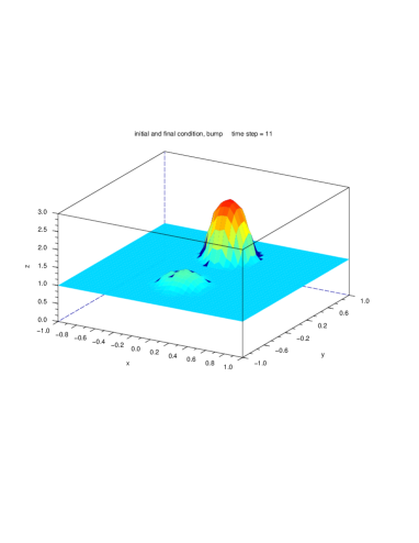
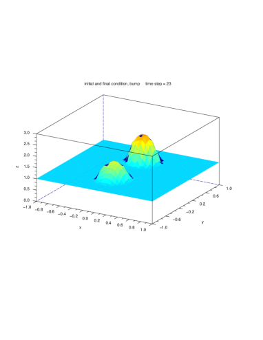
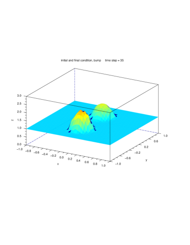
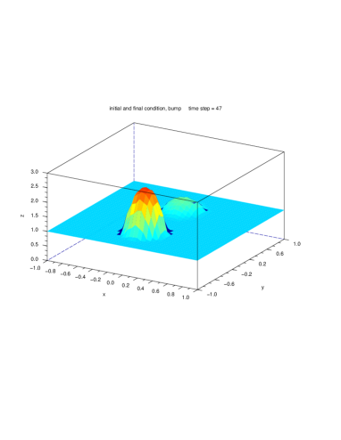
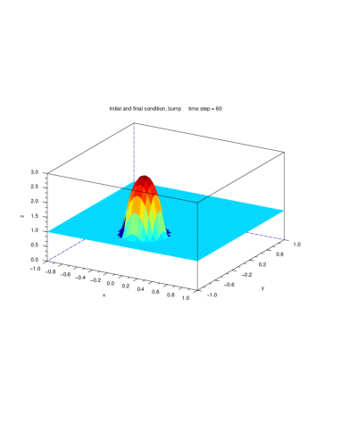
Figure 1: Bump transport for $\beta=1$

Then figures 2, 3, 4, and 5 describe the bump transport for $\beta=0.5$, $0.2$, $0.1$, and $0.05$.

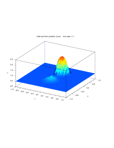
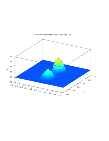
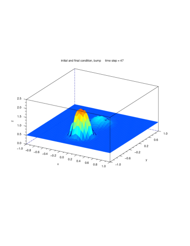
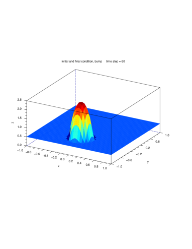
Figure 2: Bump transport for $\beta=0.5$

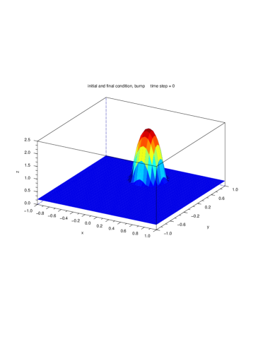
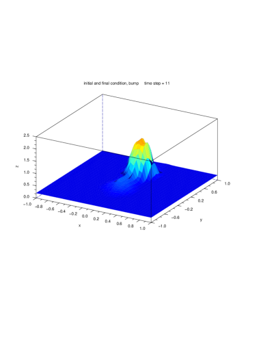
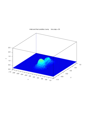
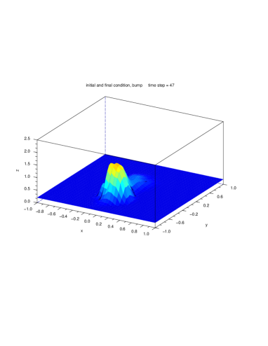
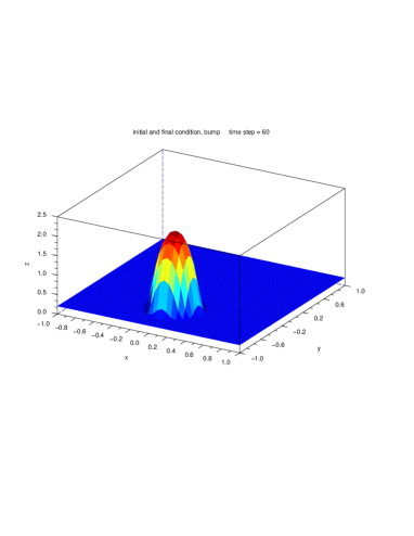
Figure 3: Bump transport for $\beta=0.2$

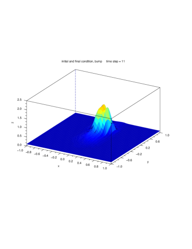
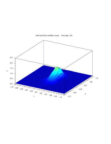
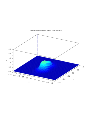
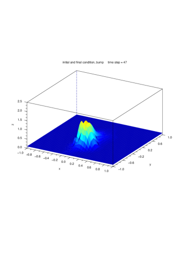
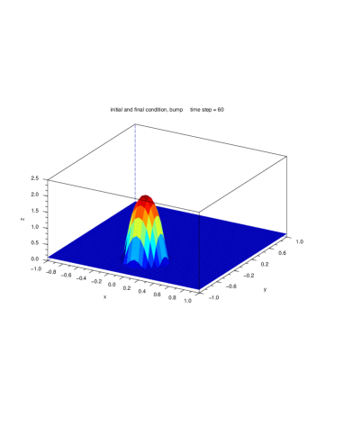
Figure 4: Bump transport for $\beta=0.1$

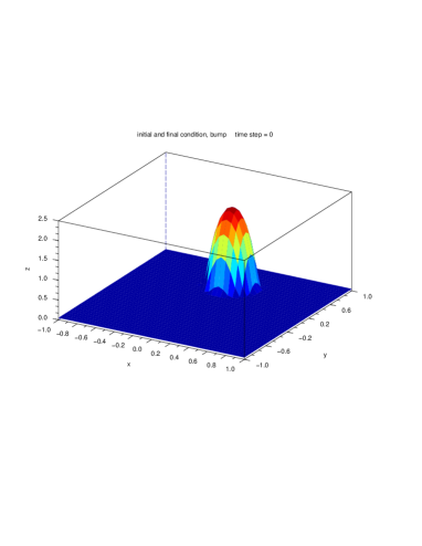
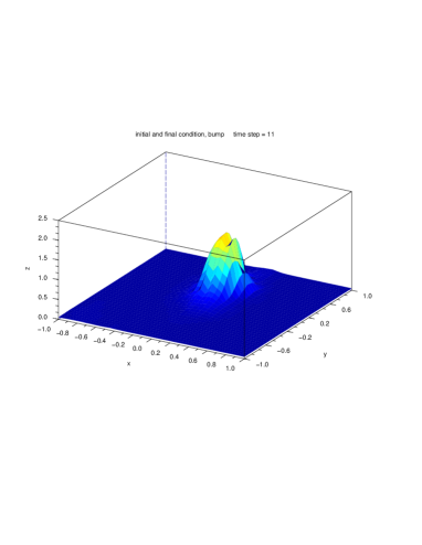
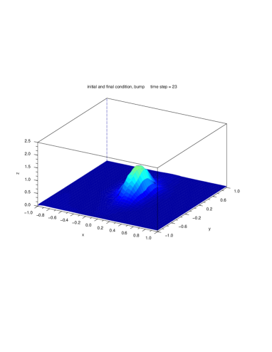
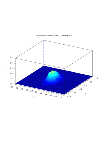
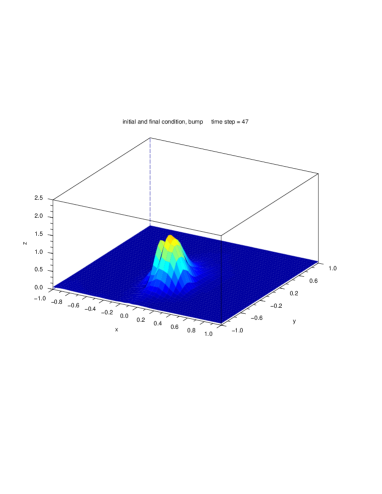
Figure 5: Bump transport for $\beta=0.05$

Remark that when $\beta$ is small, the linear system becomes very ill-conditioned. Indeed for $\beta\leq 0.1$ usual preconditioners like the classical IC0 one are useless. In this case the parallel Gram-Schmidt least squares preconditioner (DIAG + LS CGS OPT) developed in [18, 17, 19] is used. Then the linear system is solved in parallel using $48$ processors. The global tolerance for the iterative scheme developed in section 2 is set to $0.01$.

The number of iterations, and the CPU time for each value of $\beta$ is given in table 1. For $\beta<0.05$ the algorithm did not converge.

$\beta$	nb. iterations	CPU time [s]	residue
1	4	128	$8.62\,10^{-4}$
0.5	5	149	$9.23\,10^{-3}$
0.2	8	201	$4.41\,10^{-3}$
0.1	10	229	$9.47\,10^{-3}$
0.05	55	1019	$7.77\,10^{-3}$

Table 1: CPU time and number of iterations

4.2 The left ventricle motion

The iterative strategy described in Section 2 is then used to compute an approximated solution, and to reconstruct the systole to diastole images of a slice of a left ventricle. Ten time steps have been used to compute the solution, and 10000 degrees of freedom for the time-space least squares finite element. The approximated fixed point algorithm converges in about 10 iterations with an accuracy of about $10^{-4}$. In this case the usual IC0 preconditioner is sufficient; this is essentially due to the fact that there is no large region in the domain with a very low density $\rho$. In the next figure 6, the initial image and the final image are presented.

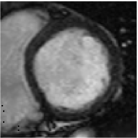
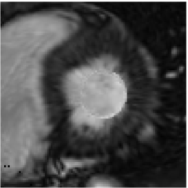
Figure 6: End of diastole of a left ventricular (a), of systole (b)

In the following figure 7, two intermediate times $1/3$ and $2/3$ are shown.

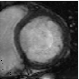
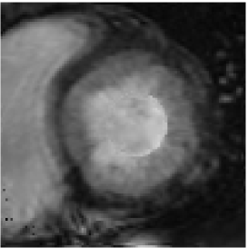
Figure 7: Time step 3 and 6

To summarize, in this work, we present a fixed point algorithm for the computation of the time dependent optimal mass transportation problem, allowing to handle the images tracking problem. The efficiency of the method has been tested with some 2D examples.

References

• [1] L. Ambrosio, Transport equation and Cauchy problem for BV vector fields. Invent. math. 158, 227-260, (2004).
• [2] J.P. Aubin, Viability theory. Birkhauser, (1991).
• [3] S. Angenent, S. Haker and A. Tannenbaum, Minimizing Flows for the Monge-Kantorovich Problem, SIAM J. Math. Anal. 35, 61–97, (2003).
• [4] G. Aubert, R. Deriche and P. Kornprobst, Computing optical flow problem via variational techniques. SIAM J. Appl. Math., 80, 156–182, (1999).
• [5] J. Benamou and Y. Brenier, A computational fluid mechanics solution to the Monge-Kantorovich mass transfer problem, Numer. Math., 84, 375–393, (2000).
• [6] J. Benamou,Y. Brenier and K. Guittet, The Monge-Kantorovich mass transfer and its computational fluid Mechanics formulation. Int. J. Numer. Math. Fluids 40, 21–30, (2002).
• [7] O. Besson and J. Pousin, Solutions for linear conservation laws with velocity fields in $\mathit{L}^{\infty}$. Arch. Rational Mech. Anal., 186, 159–175, (2007).
• [8] O. Besson and G. de Montmollin, Space-time integrated least squares: a time marching approach. Int. J. Numer. Meth. Fluids, 44, 525–543, (2004).
• [9] P.B. Bochev and M.D. Gunzburger, Least-Squares Finite Element Methods, volume 166, Applied Mathematical Sciences, Springer, 2009.
• [10] B. Dacorogna and J. Moser, On a partial differential equation involving the Jacobian determinant, Ann. Inst. Henri Poincaré, 7, 1–26, (1990).
• [11] B. Delhay, P. Clarysse and I.E. Magnin, Locally adapted spatio-temporal deformation model for dense motion estimation in periodic cardiac image sequences, In Functional Imaging and Modeling of the Heart, volume LNCS 4466, Salt Lake City, UT, USA, 393–402, (2007).
• [12] B. Delhay, J. Ltjnen, P. Clarysse, T. Katila, I. E. Magnin, A Dynamic 3-D Cardiac Surface Model from MR Images. Computers In Cardiology, (2005).
• [13] D. Gilbarg, N.S. Trundinger, Elliptic Partial Differential Equations of Second Order. Springer, (2001).
• [14] M. Lynch, O. Ghita and P. F. Whelan, Segmentation of the Left Ventricle of the Heart in 3D+t MRI Data Using an Optimized Non-Rigid Temporal Model, IEEE TMI Issue 2, 195–203, (2008).
• [15] M. Picq, Résolution de l’équation du transport sous contraintes. PhD thesis, INSA Lyon (2007).
• [16] J. Schaerer, P. Clarysse, and J. Pousin, A New Dynamic Elastic Model for Cardiac Image Analysis. In Proceedings of the 29th Annual International Conference of the IEEE EMBS, Lyon, France, 4488–4491, (2007).
• [17] J. Straubhaar. Preconditioners for the conjugate gradient algorithm using Gram–Schmidt and least squares methods. Internat. J. Comput. Math., 84(1):89–108, 2007.
• [18] J. Straubhaar. Préconditionnement de systèmes linéaires symétriques définis positifs. Application à la simulation numérique d’écoulements océaniques tridimensionnels. PhD thesis, Université de Neuchâtel, 2007.
• [19] J. Straubhaar. Parallel preconditioners for the conjugate gradient algorithm using Gram–Schmidt and least squares methods. Parallel Comput., 34(10):551–569, 2008.
• [20] C. Villani, Topics in optimal transportation. Amer. Math. Soc. Providence, Graduate Studies in Mathematics 58, (2003).