Geometrical Aspects on Parameter estimation of stochastic gravitational wave background: beyond the Fisher analysis
Abstract
The maximum likelihood method is often used for parameter estimation in gravitational wave astronomy. Recently, an interesting approach was proposed by Vallisneri to evaluate the distributions of parameter estimation errors expected for the method. This approach is to statistically analyze the local peaks of the likelihood surface, and works efficiently even for signals with low signal-to-noise ratios. Focusing special attention to geometric structure of the likelihood surface, we follow the proposed approach and derive formulae for a simplified model of data analysis where the target signal has only one intrinsic parameter, along with its overall amplitude. Then we apply our formulae to correlation analysis of stochastic gravitational wave background with a power-law spectrum. We report qualitative trends of the formulae using numerical results specifically obtained for correlation analysis with two Advanced-LIGO detectors.
pacs:
PACS number(s): 95.85.Sz 95.30.SfI Introduction
Nowadays, large-scale ground-based laser interferometers such as LIGO Harry:2010zz , Virgo Accadia:2011zzc and KAGRA (formerly LCGT) Kuroda:2011zz , are being upgraded or constructed to realize powerful second generation detectors. It is expected that we will succeed to directly detect gravitational waves (GWs) around 10-1000Hz in this decade. Subsequently, the Laser Interferometer Space Antenna (LISA) lisa (see also AmaroSeoane:2012km for eLISA/NGO) will explore a new window of GWs around 0.1-100mHz. At the lower frequency regime nHz, the pulsar timing arrays Manchester:2011ec ; Hobbs:2009yy have been significantly improving their sensitivities to GWs.
Under these circumstances, possibilities of GW astronomy have been actively discussed for these projects, and extracting parameters characterizing GWs is widely recognized as one of the most important tasks. To evaluate the accuracy of parameter estimation, the Fisher matrix approximation is a standard tool and often used in these studies thorne ; Finn:1992wt ; Cutler:1994ys ; jk . This method is quite simple to implement, but its performance is known to become worse at lower signal-to-noise ratios (SNRs) Vallisneri:2007ev . Unfortunately, a full numerical study mimicking actual data analysis requires a huge computational cost. To fill the gaps between these two methods, Vallisneri Vallisneri:2011ts recently proposed an interesting and efficient method to predict distributions of the parameter estimation errors expected for maximum likelihood analyses. He noticed that the mean densities of the local stationary points (peaks, valleys and saddle points) of a likelihood surface can be handled relatively concisely under fluctuations of the surface induced by the detector noises. This is because (i) the dependence of the relevant expressions on the noises is rather simple and (ii) only a small number of independent noise components is involved. In his work, it was suggested that the new method can well reproduce the costly results obtained by fully numerical methods. He also commented that the proposed method can be utilized to analyze multiple local peaks, including not global ones that could cause troubles at the actual parameter estimation. In this paper, we examine this direction, paying attention to geometrical properties of likelihood surfaces, not only their local peaks but also valleys and saddle points.
As a first step, our target is limited to a simple model where we estimate only one intrinsic parameter and the overall amplitude of the signal (thus at most two fitting parameters). While we cannot analyze important issues inherent to large dimensionalities of fitting parameters, our study would elucidate basic aspects of parameter estimation with the maximum likelihood method.
In this paper, we first present a formal analysis to write down the expected densities of local stationary points of a likelihood surface. Here we assume Gaussian noises, but do not specifically limit our analysis to GW observation. Then we apply our formal results to correlation analysis of stochastic GW background. We assume a power-law spectrum for the background and discuss estimation of the spectral index and the overall amplitude. Many theoretical models of the background predict power-law spectra, reflecting cosmological or astrophysical scale-free processes relevant for generation of GWs, and therefore the assumptions on the spectral shape would be reasonable at least in the frequency band of a detector (see e.g. Maggiore:1999vm ; Phinney:2001di ; Kuroyanagi:2008ye ; Nakayama:2008ip ; Alabidi:2012ex ). Therefore, the spectral index and the amplitude would be the primary parameters of a background and serve as the key information to discriminate its origin. Since the SNR of the correlation analysis increases with the observation time as Flanagan:1993ix ; Allen:1997ad , we initially need to deal with a low SNR data. This fact may reduce the validity of the Fisher matrix analysis for the early era of GW astronomy. Given these aspects, our simple analysis by the new method with one intrinsic parameter is not just a toy model, but firmly has a suitable and realistic application.
As a concrete model, we examine the correlation analysis with the two Advanced LIGO detectors and evaluate the expected number densities of the local stationary points of the maximum likelihood surface in our parameter space. These results would be useful to discuss the prospects of stochastic GW background measurements with LIGO, and also helps us to grasp qualitative trends of the formal expressions.
We find that, for moderate signal strength , there would be vanishingly low probabilities to have multiples peaks on the likelihood surfaces around the true parameters of the GW background. In contrast, false peaks arise mainly by noises at the distant parameter regions where the true signal loses correlation. They typically have low likelihood values and will be safely excluded by setting an appropriate threshold on the likelihood value. We also discuss biases of the fitting parameters estimated with the maximum likelihood method. For , the biases asymptotically decrease as relative to the true parameter and would be buried beneath the parameter estimation errors ().
This paper is organized as follows; in §II we briefly discuss parameter estimation with the maximum likelihood method. In §III, we provide formal expressions for densities of the local stationary points. §IV is devoted to link the results in §III to the correlation analysis for stochastic GW background. In §V, we evaluate the densities of the stationary points for the two Advanced LIGO detectors and report the observed trends. We also compare the traditional Fisher matrix approximation with the new predictions. §VI is a summary of this paper.
II parameter estimation
In this section, we briefly discuss a simplified model of data analysis, particularly estimation of characteristic parameters contaminated by instrumental noise. Our data are given by a real vector with its dimension , and each element ( runs from 1 to ) consists of the mean value and the noise as
| (1) |
Throughout this paper, the noise is presumed to have a Gaussian distribution with zero mean and variance . It is also assumed that each pair of the noise components has no correlation, i.e.,
| (2) |
where the bracket means the ensemble average.
We define the inner product between two real vectors and with their dimension by
| (3) |
The probability distribution function for the noise is expressed using this inner product as
| (4) |
where and . Hereafter, we omit the subscript of the vector component for simplicity, whenever we expect that the confusion of the vector component and the vector itself may not arise.
In this study, candidates of our target signal are assumed to have the form
| (5) |
where is the overall amplitude and is the template vector characterized by a single intrinsic parameter, . The template is chosen to be a unit vector, so that it satisfies the normalization condition
| (6) |
According to the definition described above, the amplitude parameter is identical to the optimal SNR of the data , and has a clear meaning. In particular, we assign and (t: suffix for the true value) for the parameters of the true signal as
| (7) |
where . While we basically consider the case in which , such as a positive-definite power spectrum in §IV, we will also provide relevant expressions for general cases with unconstrained signature of , which may be useful for the analysis of more general aspects, such as the gravitational-wave polarization.
Our primary task in the data analysis is to estimate the true parameter of the target signal from the contaminated data,
| (8) |
which we can observe in reality. A standard and efficient prescription is the likelihood analysis, in which template families are prepared to fit the data. In this study, the template is given by with two parameters , and we define the inner product
| (9) |
which is closely related to the distance 111The distance should be defined by . between the data and the template . For a given noise vector , we regard as a continuous function on the two dimensional plane , and search the point where the function takes the globally maximum value in the data analysis. Here, the subscript “bf” stands for “best fit.”
The inner product is a quadratic function of the amplitude , and can be written as
| (10) |
The first term is the only term dependent on , and we can always set this term to zero by appropriately choosing . Therefore, we initially search the index where the inner product takes its global maximum 222Actually, the global maximum of the function is at the parameter with maximum . But our concrete model for GW backgrounds analyzed in this paper has a physical requirement (as already assumed). Therefore, we mostly analyze the simple form instead of . But we briefly revisit this issue in §III., and assign the best-fit amplitude as
| (11) |
This procedure is essentially the same as the matched filtering analysis with the normalized templates and the Wiener filter (see e.g. thorne ). The simple relation Eq. (11) between the amplitude and the peak value turns out to be useful later. Hereafter, we omit the argument of and for simplicity. The subscripts “” and “” represent the dimensions of the fitting parameters (“” for the single parameter and “” for the two parameters ).
The estimated values depend on specific realization of the noise , and are scattered around the true values . Therefore, they should be regarded as statistical variables fluctuating in response to the realizations of the noise vector . Our primary interest in this paper is the probability distribution function of the estimated parameters .
At the global solution obtained for a given noise vector , the function meets the following relations required for a local peak,
| (12) |
as necessary conditions 333 The simple expressions in this paper are given for data analysis with a single intrinsic parameter . If there are totally intrinsic parameters , the local peaks of the function are the stationary points where all the eigenvalues of the Hesse matrix are negative.. However, the local relations Eq. (12) are not the sufficient conditions for the global maximum of the function , as it might have multiple peaks for a single realization of the noise . With multiple peaks, it is necessary to select the global maximum in actual data analysis.
Nevertheless, it was shown in Vallisneri:2011ts (see Fig.3 in the paper) that numerical results for distribution of the global peaks of likelihood surfaces can be reproduced well by a local expression that actually counts the stationary points of the surfaces. Based on this observation, the aims of this paper are (i) to geometrically develop an analytical framework for the local peak statistics in simplified one-dimensional cases, and (ii) to apply it for the correlation analysis of GW backgrounds, as a realistic example.
In our local approach, we unavoidably count the contribution of more than one peaks of the function . In general, it is difficult to analytically handle global properties of complicated functions (see e.g. adler ). On the other hand, between two adjacent peaks of a one-dimensional function, we must have a valley (local minimum) with the relations
| (13) |
because of the continuity of the function . These two are local conditions, and can be managed analytically. We thus analyze the distribution of the valleys that would supplementary help us to discuss the multiplicity of the solutions for the local peaks Eq. (12).
Next, based on the above discussions on the peaks and valleys of the one-dimensional function , we expand our considerations to the local geometry on the two-dimensional surface . Here, it should be noted that the cross section of the surface at a fixed parameter has a parabolic shape convex upward with . Therefore, no local minimum on the two dimensional surface appears. Indeed, the parabolic shape along the amplitude is the universal feature of any dimensional likelihood surface as long as normalized template families are adopted.
For a solution of the local peak conditions Eq. (12), we assign the corresponding amplitude by . Then, the function turns out to have a local peak at as easily seen from Eq. (10). In the same manner, we can assign the amplitude for a solution of the local valley conditions Eq. (13). Although the function becomes a saddle point (not a local minimum) at the point , we continue to use the suffix “vl” originally defined for the valleys of the one-dimensional function in this two-dimensional case.
Although we only deal with the real data in this paper, it is straightforward to expand our formalism for complex data with random Gaussian noises. For complex vectors and , the inner product Eq. (3) should be modified as
| (14) |
and the elements and should be modified to include both real and imaginary contributions of the noise, . The amplitude should also be regarded as a complex variable, and we can still make similar arguments for parameter estimation based on the relation
| (15) |
III Densities of local peaks
As commented earlier, our data contain the noise that results in fluctuating the positions of the local peaks. Now, let us consider an ensemble of the noise vectors whose probability distribution function is given by Eq.(4). For each realization of the noise vector , we can pick up all the local peaks for the fluctuated function . Here the total number of the local peaks is not necessarily unity. Next, for the ensemble of the noises vectors, we statistically handle the spatial distributions of the local peaks. In this manner we can evaluate the expected number of the local peaks in a small parameter range and express it in the form
| (16) |
Due to its definition, we can regard as the expected number density of the local peaks.
Similarly, we put the expected number of the local peaks for the function in a two dimensional region by
| (17) |
with the corresponding number density . In this section, basically following Vallisneri:2011ts , we derive analytical expressions as well as for the expectation values of the local peaks. Considering potential multiplicity of the local peaks, we call these functions as densities, rather than the probabilities (that should be normalized to unity).
Here it is important note that (i) the global peaks are sub-classes of the local peaks and (ii) our density distributions and would provide upper limits for the probability distributions of the global ones. In the same manner, we denote the expected number densities of local valleys (and saddles) by and .
In this section, we do not use the concrete form of the normalized template . Therefore, our results in this section can be generally applicable for estimation of a single parameter and the associated amplitude , through the relation (10) under presence of Gaussian noises.
III.1 formal expressions
First, we introduce the simplified notations () below
| (18) |
for the derivatives of the unit template vector with for .
For a given noise vector , we can count the number of the local peaks in the parameter range for the function as (see e.g. Vallisneri:2011ts ; adler ; Bardeen:1985tr )
| (19) |
where is the delta function and we defined the function
| (20) |
In Eq.(19), the delta function represents the condition for the extremum , and we temporarily recover the argument for the function in order to clarify its dependence on the noise. The function selects the sign appropriate for a peak, and also fixes the measure associated with the delta function. Taking account of the probability distribution of the noise , the expected number of the local peaks is given by
| (21) |
or equivalently
| (22) |
In the same manner, the density of the local valleys is given by
| (23) |
As for the two dimensional density distribution of the local peaks and saddles (with the subscript “vl”), we have similar expressions
| (24) |
and
| (25) |
The above expressions (22)(23)(24) and (25) are written as multidimensional integrals for the noise vector . However, for a given parameter , only the following three inner products and are relevant in Eqs.(24) and (25). For Eqs.(22) and (23), we need to deal with only the two combinations and .
The variables , and are specific linear combinations of the large-dimensional vector . Therefore, the actual dimensions of the integral can be reduced down to 3 or 2 Vallisneri:2011ts . If the each component of the noise vector is Gaussian, the probability distribution function is completely determined by their covariance matrix . From the definition of the inner product, we have
| (26) |
where we defined
| (27) |
From the normalization of the templates, we readily have and . We also define the product between the vector and the unit vector for the true index as
| (28) |
Integrating out irrelevant noise elements in Eq.(22), the density is given by
| (29) |
While we can directly manage this expression, the covariance between and is somewhat cumbersome for polynomial deformations 444We can use the functional freedom of the parameter to simplify the covariance matrix for the noises. More specifically, we introduce the new parameter with the relation Then we have and . Here the quantities with the prime ′ are given for the new parameter . The only non-trivial one is written with the original ones (for the parameter ) by . We can easily deal with the probability distribution function of the related noise matrix due to the simple structure of the correlation without using the additional vector . Once we derive the density for the new variable . The density for the original parameter is given by .. Below, we take a different route by introducing the new unit vector defined by
| (30) |
that satisfies and is orthogonal to the vector as .
The original vector is given by and as
| (31) |
We hereafter use instead of , and define the products and by
| (32) |
They are given by the products and as
| (33) |
and
| (34) |
We also introduce the new stochastic variable as
| (35) |
We have and . Then the covariance matrix between is given by
| (36) |
Taking inverse of the relevant parts of the matrix, we have the probability distribution functions as
| (37) |
and
| (38) |
From the formal expression (22), we eliminate the variables and using Eqs.(34) and (35), and obtain
| (39) |
By performing the -integral first, we find
| (40) |
with
| (41) | |||||
| (42) | |||||
| (43) |
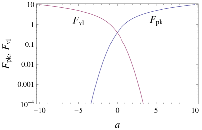
Here, the first factor originates from the delta function for a stationary point, and is closely related to the Fisher matrix prediction (see the next subsection). In Eq.(43) we used the complementary error function . In the same manner we obtain the density of the local valleys as
| (44) |
with
| (45) |
The two functions and are plotted in Fig.1. We can easily derive the following relations
| (46) |
We have for the relative abundances of the peaks and valleys. The number of peaks dominates that of the valleys at .
The two dimensional density profiles and can be evaluated similarly as
| (47) | |||||
| (48) |
and we have the following identity between and
| (49) |
due to the simple structure for the amplitude parameter .
While we have introduced the orthogonal vector to simplify the covariance noise matrix (36), we can directly reach Eqs.(40)(44) and (47) from the original expressions (22)(23) and (24).
We evaluate the mean value of the peak amplitude as follows
| (50) | |||||
| (51) |
Here the first term is the simple average of the product with respect to the noise . The second one is a positive definite term with a negative factor , and represents the bias caused by selecting only peaks. Due to the negative correlation between the two noise components and , the requirement for being a peak (related to ) introduces the bias for the product .
As mentioned earlier, at actual data analysis, we initially search the point where the product takes the global maximum. Even if our target points are shifted to the local peaks of the function , instead of the global peak, it is expected that the product would take relatively large values for local peaks around the true parameter but smaller values for those generated merely by statistical fluctuations at points distant from . In this manner, the magnitude of the product at a local peak would become in itself an useful indicator for our theoretical analysis purely based on local quantities. Here we introduce the notation for the value of at a local peak and distinguish it from the original one-dimensional function .
We thus consider the expected number of local peaks in the parameter range and the peak height , and denote it by . Following the arguments around Eqs.(19)-(22) we have
| (52) |
But the expression (52) is essentially the same as Eq.(24)
| (53) |
due to the simple correspondence between the estimated amplitude and the inner product as shown in Eq.(11). Therefore, we can use the density distribution also for the function . Once the curves and are given for two different values and , we can apply the relation (see Eq.(49)) to compare the relative densities of and by eye, based on the areas of the two curves.
The unimportant peaks due to noises at an index distant from the true value would mostly have low peak heights and would be efficiently removed by choosing an appropriate threshold on , as demonstrated later. To elucidate this, we define the density of local peaks above a given threshold by
| (54) |
As commented earlier, we first searched maximums of the function instead of , considering the requirement valid e.g. for the estimation of a power spectrum that is a positive definite quantity (as analyzed in the next section). If we literally evaluate the local peaks/valleys for the function without the prior , they are given with our expressions (47) and (48) as
| (55) |
respectively. Here is the step function. Similarly, the local peaks/valleys of the function are obtained as
| (56) |
Here, we should notice that the roles of peaks and valleys of the function interchange for the absolute value at . While we do not use these somewhat complicated expressions (55) and (56), these would be more adequate, depending on problems.
III.2 large SNR limit
It is well known that, with a large SNR, the distribution of the parameters estimated by the matched filtering is well approximated by the Fisher matrix predictions around their true values Finn:1992wt ; Cutler:1994ys ; Vallisneri:2007ev . In this subsection, we examine the profiles of our density distribution functions and at larger . Similar analyses were already done in Vallisneri:2011ts , but it would be instructive to directly examine our analytic expressions obtained in the previous subsection.
We first expand the fitting parameter around their true values and define the deviations as
| (57) |
Then, taking the leading order term with respect to , we obtain
| (58) |
and
| (59) |
where the product is evaluated at the point . With the asymptotic relation at , the expressions (40) and (47) for the local peaks can be approximated as
| (60) |
and
| (61) |
for small and and at .
Meanwhile we have the Fisher matrix for the two parameters and at their true values as
| (62) |
It is straightforward to confirm that the Fisher matrix predictions agree with our expressions (60) and (61) originally given for the local peaks. We hereafter denote the right-hand sides of these equations by and .
At , the Gaussian distribution is strongly localized around with the characteristic width . Therefore it would be advantageous to use the rescaled variable to analyze the shape of the function relative to . After some algebra, we can derive the following perturbative expression.
| (63) |
Here we have and the higher order term H.O. is given by a polynomial of whose coefficients are at most . The leading-order correction term is given by
| (64) |
Thus, with the rescaled variable , the difference asymptotically approaches the fixed function at . In the next section, we demonstrate this numerically.
In order to characterize the shape of the function , we evaluate its zeroth, first and second moments by taking integrals. Since is an odd function, we can derive the following results;
| (65) | |||||
| (66) | |||||
| (67) |
These would be used in §V.D. Due to the normalization condition (65), the right-hand-side of Eq.(66) can be regarded as the estimation bias of the primary parameter . In the same manner, we have the bias for the mean value for the overall amplitude
| (68) |
Note that the term is a second order correction relative to the true amplitude . The parameters estimated by the maximum likelihood method generally have biases from the second order (see Vitale:2010mr for a perturbative analysis) and those in Eqs.(66) and (68) agree with results obtained from perturbative expressions for the effects of the noises (e.g. Eq.(A31) in Cutler:1994ys ).
IV correlation analysis for stochastic GW backgrounds
Hereafter, we apply our formal studies to correlation analysis of gravitational wave background Flanagan:1993ix ; Allen:1997ad . In this section, we first describe basic aspects of the correlation analysis, and mention its correspondence to the data analysis prescription discussed in §II and III. Then we provide expressions that would be useful for numerically evaluating the local peak/valley densities for parameter estimation of GW backgrounds with power-law spectra.
IV.1 data correlation
We discuss observation of an isotropic stochastic GW background with two L-shaped detectors and in an observational period . The Fourier modes of two data streams are linear combinations of the responses to the background signal and the detector noises as
| (69) |
We assume that the detector noises and are stationary with no correlation between them (namely ). We define the noise spectra of the two detectors and in the following relations
| (70) |
The responses and to the GW background would have correlation that is characterized by the overlap reduction function as
| (71) |
where is the energy density of the GW background in the logarithmic frequency interval and normalized by the critical density of the universe (: the Hubble parameter hereafter fixed at 70km/sec/Mpc). The overlap reduction function depends strongly on the relative configuration of the two detectors and is given by the following angular integral Flanagan:1993ix ; Allen:1997ad
| (72) |
with the beam pattern functions and the spatial positions of detectors . We have the upper limit valid for co-aligned detectors.
In this article we study the situations where the observational data is dominated by the detector noises () as
| (73) |
(weak signal condition). Under this condition, the correlation analysis becomes an efficient approach to examine a weak GW background.
Following the prescription described in Seto:2005qy , we divide the observational frequency band into finite segments ( : the suffix for the segments) that have the widths and the central frequencies . The widths are selected to satisfy so that, in each segment, (i) there are a large number () of Fourier modes, and (ii) the frequency dependencies can be neglected () for the functions, such as , , and . These two conditions hold for the laser interferometers such as LIGO Harry:2010zz , Virgo Accadia:2011zzc , KAGRA Kuroda:2011zz , BBO Corbin:2005ny ; Harry:2006fi and DECIGO Seto:2001qf ; Kawamura:2006up , but not for the pulsar timing experiments which are sensitive at . Meanwhile, we have for independent data streams of LISA Prince:2002hp ; Krolak:2004xp .
To statistically amplify the target background signals and compress the data, we take the summation of the data products in each segment as
| (74) |
Here we decompose in terms of its mean value and statistical fluctuation with zero mean as
| (75) |
At this stage, we do not need to be aware of the relation between notations introduced here and in §II and III. From Eq.(71) the mean is given by
| (76) |
Note that the mean value of the summation is a real number even without the operator in Eq.(74). This is the reason why we took the real part of the product in Eq.(74) to dispose the irrelevant imaginary part of the fluctuation . With the weak signal condition, the fluctuation is dominated by the detector noises and its variance is given by
| (77) |
In the last expression, we had an additional factor 1/2 associated with the operator in Eq.(74). The product at a single frequency would not be Gaussian distributed. However, due to a large number of involved modes in a segment and the central limit theorem, the fluctuations for the compressed data can be regarded as Gaussian.
Given the noise level , we can evaluate the SNR of each segment as
| (78) |
Then the total SNR is given by a quadratic summation of all the segments
| (79) |
Note that the final expression (79) does not depend on the details of the segmentation, and agrees with those in the literature Flanagan:1993ix ; Allen:1997ad . The total SNR in Eq.(79) is also expressed as
| (80) |
with the product defined in Eq.(3). Now the vectors introduced in this section can be directly regarded as those in §II and III. Here, the dimension of the vectors is the number of the segments .
In this paper, as concrete models, we only deal with the background spectra given in a power-law form
| (81) |
in the frequency band observed by the detectors in interest. Here is the spectral index in the band, and serves as the single intrinsic parameter in the previous sections. For the mean value of the correlation analysis (see Eq.(76)), we define the unit vector whose components (including sign information) are given as
| (82) |
with the normalization condition . Introducing the additional parameter for the amplitude of a GW background, we express the mean value of the correlated data due to the background as 555While we have the physical requirement , we do not impose the corresponding (and also other) priors for simplicity.. We can now apply the formal expressions derived in §III.
In this paper, we only study the weak signal case with two available detectors. But the expression (79) can be extended for stronger GW backgrounds by the following replacement Allen:1997ad
| (83) |
For correlation analysis with more than two independent detectors, the optimal SNR is given by a summation of Eq.(79) with respect to all the possible pairs of detectors.
Hereafter, for notational simplicity, we omit the subscripts and for our two detectors, and use expressions, such as .
IV.2 shape function
As shown in Eqs.(40)(44) and (47), our expressions for the local peaks and valleys are given by the inner products and (see Eqs.(27) and (28) for their definitions). Here, note that, with Eqs.(33) and (34), the parameters and are written in terms of and . In this section, we provide simple formulae that would be easily applicable when numerically evaluating the basic ingredients and for the power law spectra , as in the next section.
Since and are defined by the inner products of two unit vectors and their derivatives with respect to the spectral indexes (see Eqs.(27) (28) and (82)), they should be generated from the integrals
| (84) |
and its (up to the fourth) derivatives with the parameter . Therefore, we define the following five functions ()
| (85) |
Here the frequency is a characteristic frequency in the observational band in interest, and should be set arbitrarily. For convenience at later discussions, we fix the normalization factor by the condition
| (86) |
or equivalently put
| (87) |
Once the lowest-order function is given numerically (e.g. with a fitting formula as in the next section), we can generate other ones (for ) by taking derivatives as
| (88) |
We call as the shape function. This function depends on the profile of the noise spectra , the overlap reduction function , and the selected frequency . Under the simple geometrical representation for the signal vector with the amplitude parameter , most of the principal information relevant for our analyses is included in the shape function.
Now we express the product in terms of . Here we need to call the functions only at , and define
| (89) |
to simplify our expressions. After some algebra, we can derive
| (90) |
These combinations do not depend on and , as expected from the simple geometric meanings of the normal vectors.
In order to evaluate related to the true vector , we similarly define the elements and by
| (91) |
Then we have
| (92) |
So far, we have used the parameter to represent the amplitude of the background. This is a geometrically natural choice. But, in some cases, it might be preferable to put the background spectrum in the form
| (93) |
and use the combination of the parameters for discussing prospects of correlation analysis, instead of the original one . Below, we summarize expressions related to these two parameterizations. From Eq.(79), the two amplitudes and are related by
| (94) |
Since the shape function is normalized as
| (95) |
we have
| (96) |
with a constant factor that is determined by the noise spectra and the overlap reduction function as
| (97) |
From the basic property of the delta function, the density of the local peaks in the parameter space is expressed with the density defined for the original space as
| (98) | |||||
| (99) |
V correlation analysis with the Advanced LIGO
In this section, we evaluate our analytical expressions for the two 4km Advanced-LIGO detectors, as a concrete example of correlation analysis for stochastic gravitational wave backgrounds. Throughout this section, we set the characteristic frequency at
| (100) |
for our power-law spectrum .
V.1 basic quantities
Our aim in this subsection is to provide the shape function and related quantities for the two Advanced LIGO detectors. These are the preliminary calculations used for our main results given in the following subsections.
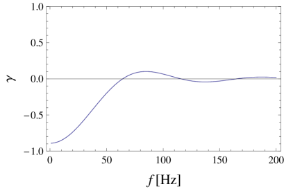
First, the overlap reduction function in Eq.(72) is expressed analytically as Flanagan:1993ix ; Allen:1997ad (see also Seto:2008sr ; Nishizawa:2009bf for polarized modes)
| (101) |
The parameter is the angle between the two detectors measured from the center of the Earth, and characterizes the orientations of the detectors relative to the great circle connecting the two sites. The variable is given by
| (102) |
with the distance (km: the radius of the Earth). The two functions and are written as
| (103) |
| (104) |
with the spherical Bessel functions . We have the upper limit and the equality here holds only for two co-aligned detectors (mod ) at a same place ( and ).
For the two LIGO detectors, the angular parameters are , and , and we show the function in Fig.2. Due to their arranged configuration, we have relatively large value at the low frequency regime . The magnitude decreases at Hz, where the wavelength of gravitational waves becomes comparable or smaller than the separation between the two detectors.
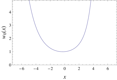
For the noise spectra of the Advanced LIGO detectors, we use a fitting formula for their broadband configuration given in Table.1. Now, the functions () can be numerically evaluated with Eq.(87), and the shape function is presented in Fig.3. Because of our choice at Hz, the curve is nearly flat around . For convenience at reproducing our numerical results below, we provide a fitting formula for the shape function
| (105) | |||||
valid in the range . While we use more accurate interpolation method for the functions throughout this paper, even the fourth derivative well approximates the accurate result with error less than 0.5% in the range .
| frequency regime [Hz] | noise spectrum |
|---|---|
| otherwise |
We also evaluate the factor defined in Eq.(97) and obtain the scaling formula
| (106) |
for the two Advanced LIGO detectors. This equation relates the amplitude of the spectrum with the SNR .
V.2 correlation functions
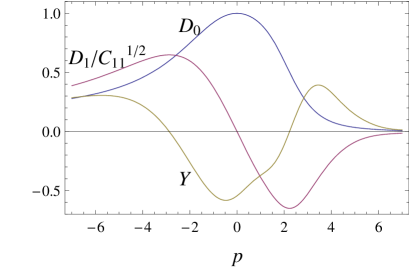
From the numerical results (), we can calculate the products and using the expressions in §IV. In this subsection, we evaluate various correlation functions that appear in our analytical expressions for the local peaks/valleys densities presented in §III. Hereafter we assume that the true GW background has a flat spectrum (namely, ).
As discussed in §II.B, the inner product between the data and the normalized template is given by the mean value and the noise part as
| (107) |
where we explicitly show the dependence on the spectral index as
| (108) |
The mean value is identical to the correlation between the true unit vector and the trial template . As shown in Fig.4, this function takes the maximum value at , and approaches 0 at larger . In the same figure, we also show the quantities and . These directly appear in the expressions for the peak/valley densities and (see Eqs.(40) and (44)), and also approach 0 at large . The parameter characterizes the relative abundances of the local peaks and valleys through the functions and , and they take similar densities at .
Around the true value , we have . At , we need a high- noise to make a valley by inverting the sign of the second derivative of the product against the background level (see Eq.(39) for a related expression). This results in a significant reduction of the valley density around , compared with the peak density , as shown in the next subsection.
In Fig.4, we took the plot range up to where the GW backgrounds become extremely blue or red, and, at these ends, it would be unreasonable to assume a single power-law spectrum in the whole LIGO band. But results in these regime would be instructive to see qualitatively how the correlation between the data and the templates affects the abundances of the local peaks and valleys.
The variance of the noise becomes unity , and its correlation at different points and is presented in Fig.5. The cross-section view at is identical to the function shown in Fig.4.
V.3 densities of local peaks/valleys
Now we evaluate the statistical formulae for the local peaks/valleys derived in §III.A. Hereafter, we use the expressions (40),(44),(47) and (48) associated with the local peaks/valleys of the function (not Eqs.(55) and (56) defined for ).
In Fig.6, we plot the local peak density for the intrinsic signal strengths and 8. For larger , the peak density shows stronger concentration around the true value . We can also observe increment of the density around where the ratio decreases again (see Fig.4) in eq.(40) with reflecting . Notice that the exponential term of the r.h.s of Eq.(40) takes the maximum value at and the function becomes a constant at . This increment of is mainly caused by the noise, as examined later.
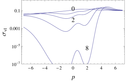
We show the density of the local valleys in Fig.6. This function is strongly suppressed by the Gaussian-like factor (see Eq.(45)) around the true value . Therefore, for signal strength , it is very unlikely that there exist multiple local peaks around , since we must have a valley between two peaks. We can further expect that the peak identified around is likely to be the global one that we want to identify at data analysis.
In order to support this from the viewpoint of the total numbers of local peaks/valleys around , we define the integrals (with the integration range selected somewhat arbitrarily) as
| (109) |
The results are shown in Fig.7. We have at , but at . The result suggests that, in principle, the spurious peaks due to the noise appear in the range . But the expected number of the peaks in the range becomes nearly unity at . The asymptotic slope is steeper than the weak bound given in Eq.(65).
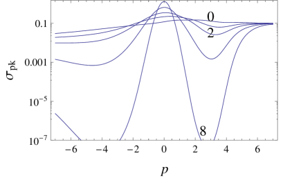
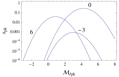
As commented earlier, the values at the local peaks themselves are the primary indicator at actual data analysis. The peak with the maximum value should be selected among multiple local peaks. The peaks existing around the true value would have relatively large values due to the underling correlation before the noise is added. We thus examine the distribution of the height of the local peaks identified at a given spectral index . In Fig.8 we plot examples of the profile (see Eq.(52)) for at the specific spectral indexes ,0 and 6. Even if two local peaks are simultaneously identified e.g. at and , the desired one would be appropriately selected on the ground of the magnitude , as far as so that peaks for true and spurious values of are likely to be distinguished (see Eq. (47)).
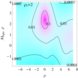
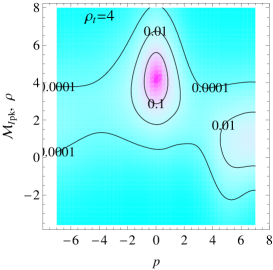
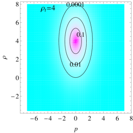
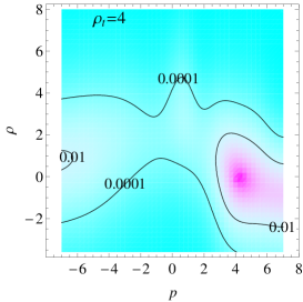
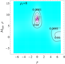
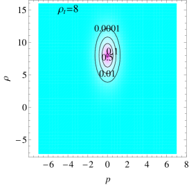
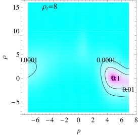
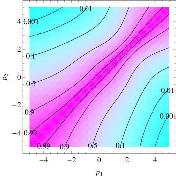
In the left panels of Fig.9, we show the two dimensional contour plots for the function (identical to and discussed later). We can observe high density region around , and an additional increment around and . The latter is due to the local peaks mainly caused by the noise. For , these two are well separated and the latter would not survive at the data analysis where we check the magnitude .
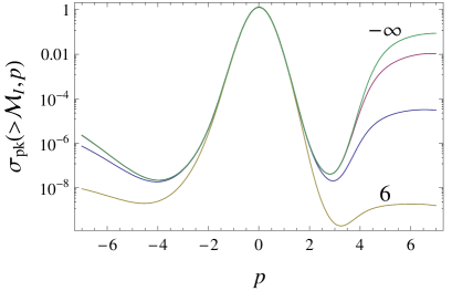
In order to show this explicitly, in Fig.10, we plot the local peak density above given threshold (see Eq.(54) for its definition). With the identity , the uppermost curve is the same as the unconstrained one given in Fig.8 for . The abundance of the local peaks around the true value is nearly the same for the four curves. But the local peaks at have the typical value and most of them are removed for the suitable threshold .
In Fig.9, the densities take their maximum values at the points with . This can be directly confirmed by putting in Eq.(47) with and , and using the monotonic shape of the function . This overestimation is closely related to the bias (see Eq.(68)) of the amplitude parameter discussed in the next subsection.
V.4 Fisher matrix predictions
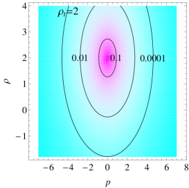
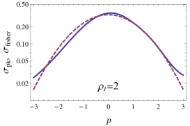
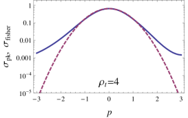
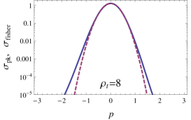
Here we compare our local peak density with the Fisher matrix prediction defined in Eq.(60). The examples are shown in Fig.11. At , the Gaussian-like profiles around the true value are similar for the two curves, and this indicates that the simple Fisher matrix prediction becomes a reasonable approximation in this regime.
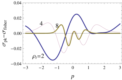
In Fig.12, we show the difference between two expressions. Since the local peak density works as an upper limit for the probability distribution function of the global peaks, the Fisher matrix predictions over estimates the probability distribution function at the spectral indexes with .
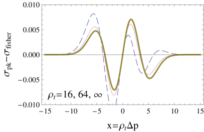
In Fig.13, we plot the function now using the rescaled parameter introduced in §III.B. As expected from the analytical evaluation, the difference approaches the leading order correction which is an odd function and characterized by two parameters and in the present case.
Next we calculate the mean and variance of the local peak distribution. To this end, we take the parameter range and renormalize the peak density as to regard it as a probability distribution function. We then evaluate the integrals
| (110) |
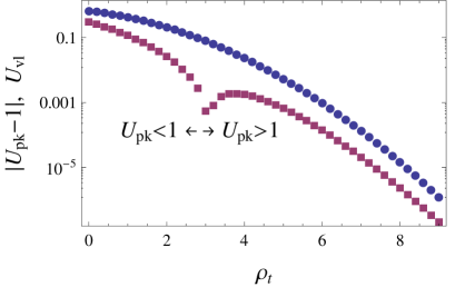
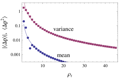
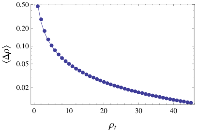
The results at various are shown in Fig.14, along with the leading order contributions () given in the left hand sides of Eqs.(66) and (67). Note that the mean value changes its sign around (from to ). The analytical curves show good agreements with the numerical ones at . Similarly, we evaluate the integral
| (111) |
for the mean bias for the amplitude parameter . In Fig.15, we plot the results with the asymptotic expression given in Eq.(68). These two also show a good agreement.
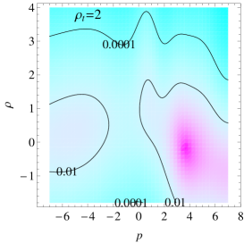
With the identity mentioned at the end of §III.A, the left panels in Fig.9 can be used to discuss the local peak distribution in the two dimensional parameter space . The overall behaviours of these figures were already described, and we do not repeat them again. But, in the middle column of Fig.9, we provide the Fisher matrix predictions. As for the one-dimensional case shown in Fig.11, the Fisher matrix predictions become good approximations for larger . In the right panels of Fig.9, we also show the density of saddle points . We can observe increment of the density around the regions where the local peak density is enhanced by the noises (especially for ). Since the intrinsic correlation is weak here, the preference of the sign is decreased and the peak/valley densities show similar patterns. In contrast, the saddle points are strongly suppressed around the true value , as mentioned earlier.
VI Summary
In this paper, we discussed a simplified model of data analysis where we estimate a single intrinsic parameter and the overall amplitude of a signal that is contaminated by Gaussian noises. The approach behind our study was recently proposed by Vallisneri Vallisneri:2011ts , and based on the fact that the local stationary points on the likelihood surfaces can be studied with a small number of independent noise components.
In this paper, we paid special attention to the local geometric aspects of the likelihood surfaces, including valleys and saddle points. With our analytic expressions derived owing to the simplified settings, we can see how the geometrical structure depend on the signal strength, the likelihood value, and correlation between the true and the trial templates. We expect that our qualitative results would provide us useful insights when dealing with more complicated problems of data analysis for GW astronomy (and beyond).
In the later half of this paper, we applied our formal expressions to correlation analysis of stochastic GW backgrounds. Considering ubiquitously realized scaling behaviours of cosmological processes (and also astrophysical ones related to GWs), it would be reasonable to assume a power-law spectrum for the background in the frequency regime of a GW detector and discuss accuracy of parameter estimation for the spectral index and the amplitude of the spectrum. Therefore, the correlation analysis for the background can be regarded as an exemplary as well as realistic case for applying our formal expressions. At the same time, this concrete example would conversely help us to see the qualitative trends of the formal results.
To link the correlation analysis with the formal results, we provided useful expressions, including ready-to-use fitting formulae for the two LIGO detectors. Then, we numerically evaluated the expected densities of the local peaks/valleys/saddle points of the likelihood surfaces. We find that the abundance of the local valleys is strongly suppressed around the true parameters, indicating prohibition of multiple peaks there. In contrast, at the region where the true signal lose correlation, there appears peaks and valleys mainly caused by the fluctuations of the noise. These false peaks would typically have low likelihood significance due to the lack of the underlying signal correlation. Therefore, they will be safely ruled out in the actual data analysis by setting an appropriate threshold on the value of the likelihood. At , the expansion around the Fisher matrix prediction to the first order in is found to approximate the exact results to a good accuracy. We also analyzed the biases for parameters estimated with the maximum likelihood method. At , our results show good agreements with those obtained in a perturbative method as second order corrections relative to the true parameters.
This work was supported by JSPS grants 20740151, 21684014, and 24540269.
References
- (1) G. M. Harry [LIGO Scientific Collaboration], Class. Quant. Grav. 27, 084006 (2010).
- (2) T. Accadia et al., Class. Quant. Grav. 28, 114002 (2011).
- (3) K. Kuroda [LCGT Collaboration], Int. J. Mod. Phys. D 20, 1755 (2011).
- (4) P. L. Bender et al. LISA Pre-Phase A Report, 1998.
- (5) P. Amaro-Seoane, S. Aoudia, S. Babak, P. Binetruy, E. Berti, A. Bohe, C. Caprini and M. Colpi et al., arXiv:1201.3621 [astro-ph.CO].
- (6) R. N. Manchester, AIP Conf. Proc. 1357, 65 (2011) [arXiv:1101.5202 [astro-ph.HE]].
- (7) G. Hobbs et al., Class. Quant. Grav. 27, 084013 (2010) [arXiv:0911.5206 [astro-ph.SR]].
- (8) K. S. Thorne, in 300 Years of Gravitation, ed. S.W. Hawking and W. Israel (Cambridge University Press, Cambridge, 1987), pp. 330-458.
- (9) L. S. Finn, Phys. Rev. D 46, 5236 (1992) [gr-qc/9209010].
- (10) C. Cutler and E. E. Flanagan, Phys. Rev. D 49, 2658 (1994) [gr-qc/9402014].
- (11) P. Jaranowski and A. Krolak, Living Rev. Relativity 8, 3 (2005).
- (12) M. Vallisneri, Phys. Rev. D 77, 042001 (2008) [gr-qc/0703086 [GR-QC]].
- (13) M. Vallisneri, Phys. Rev. Lett. 107, 191104 (2011) [arXiv:1108.1158 [gr-qc]].
- (14) M. Maggiore, Phys. Rept. 331, 283 (2000) [gr-qc/9909001].
- (15) E. S. Phinney, astro-ph/0108028.
- (16) S. Kuroyanagi, T. Chiba and N. Sugiyama, Phys. Rev. D 79, 103501 (2009) [arXiv:0804.3249 [astro-ph]].
- (17) K. Nakayama, S. Saito, Y. Suwa and J. Yokoyama, Phys. Rev. D 77, 124001 (2008) [arXiv:0802.2452 [hep-ph]].
- (18) L. Alabidi, K. Kohri, M. Sasaki and Y. Sendouda, arXiv:1203.4663 [astro-ph.CO].
- (19) E. E. Flanagan, Phys. Rev. D 48, 2389 (1993) [astro-ph/9305029].
- (20) B. Allen and J. D. Romano, Phys. Rev. D 59, 102001 (1999) [gr-qc/9710117].
- (21) J. M. Bardeen, J. R. Bond, N. Kaiser and A. S. Szalay, Astrophys. J. 304, 15 (1986).
- (22) R. J. Adler, The Geometry of Random Fields (Chichester, Wiley, 1981)
- (23) S. Vitale and M. Zanolin, Phys. Rev. D 82, 124065 (2010) [arXiv:1004.4537 [gr-qc]].
- (24) N. Seto, Phys. Rev. D 73, 063001 (2006) [gr-qc/0510067].
- (25) V. Corbin and N. J. Cornish, Class. Quant. Grav. 23, 2435 (2006) [gr-qc/0512039].
- (26) G. M. Harry, P. Fritschel, D. A. Shaddock, W. Folkner and E. S. Phinney, Class. Quant. Grav. 23, 4887 (2006) [Erratum-ibid. 23, 7361 (2006)].
- (27) N. Seto, S. Kawamura and T. Nakamura, Phys. Rev. Lett. 87, 221103 (2001) [astro-ph/0108011].
- (28) S. Kawamura et al., Class. Quant. Grav. 23 (2006) S125.
- (29) T. A. Prince, M. Tinto, S. L. Larson and J. W. Armstrong, Phys. Rev. D 66, 122002 (2002) [gr-qc/0209039].
- (30) A. Krolak, M. Tinto and M. Vallisneri, Phys. Rev. D 70 (2004) 022003 [Erratum-ibid. D 76 (2007) 069901] [gr-qc/0401108].
- (31) N. Seto and A. Taruya, Phys. Rev. D 77, 103001 (2008) [arXiv:0801.4185 [astro-ph]].
- (32) A. Nishizawa et al., Phys. Rev. D 79, 082002 (2009) [arXiv:0903.0528 [astro-ph.CO]].