The Clustering of Galaxies in the SDSS-III DR9 Baryon Oscillation Spectroscopic Survey: Testing Deviations from $\Lambda$ and General Relativity using anisotropic clustering of galaxies

Abstract

We use the joint measurement of geometry and growth from anisotropic galaxy clustering in the Baryon Oscillation Spectroscopic Survey (BOSS) Data Release 9 (DR9) CMASS sample reported by Reid et al. to constrain dark energy (DE) properties and possible deviations from the General Relativity (GR). Assuming GR and taking a prior on the linear matter power spectrum at high redshift from the cosmic microwave background (CMB), anisotropic clustering of the CMASS DR9 galaxies alone constrains $\Omega_{\rm m}=0.308\pm 0.022$ and $100\Omega_{\rm k}=5.9\pm 4.8$ for $w=-1$, or $w=-0.91\pm 0.12$ for $\Omega_{k}=0$. When combined with the full CMB likelihood, the addition of the anisotropic clustering measurements to the spherically-averaged BAO location increases the constraining power on dark energy by a factor of 4 in a flat CDM cosmology with constant dark energy equation of state $w$ (giving $w=-0.87\pm 0.05$). This impressive gain depends on our measurement of both the growth of structure and Alcock-Paczynski effect, and is not realised when marginalising over the amplitude of redshift space distortions. Combining with both the CMB and Supernovae Type Ia (SNeIa), we find $\Omega_{\rm m}=0.281\pm 0.014$ and $1000\Omega_{\rm k}=-9.2\pm 5.0$ for $w=-1$, or $w_{0}=-1.13\pm 0.12$ and $w_{\rm a}=0.65\pm 0.36$ assuming $\Omega_{k}=0$. Finally, when a $\Lambda$CDM background expansion is assumed, the combination of our estimate of the growth rate with previous growth measurements provides tight constraints on the parameters describing possible deviations from GR giving $\gamma=0.64\pm 0.05$. For one parameter extensions of the flat $\Lambda$CDM model, we find a $\sim 2\sigma$ preference either for $w>-1$ or slower growth than in GR. However, the data is fully consistent with the concordance model, and the evidence for these additional parameters is weaker than $2\sigma$.

1 Introduction

All currently available cosmological observations, including the latest datasets of CMB temperature and polarisation anisotropies (Komatsu et al., 2011), Supernovae Type Ia (SNeIa) magnitudes (Suzuki et al., 2012) and the distance ladder mapped by Baryon Acoustic Oscillation (BAO) peak signature in the clustering of galaxies (Anderson et al., 2012) are consistent with a simple cosmological model in which general relativity (GR) describes gravitational interactions on all scales and times, about 70 per cent of the Universe’s current energy density is in form of a Cosmological Constant as originally described by Einstein, and most of the remaining 30 per cent is in form of nonrelativistic “dark matter” (For a detailed review see e.g., Peebles & Ratra, 2003; Weinberg et al., 2012).

Ongoing and future observations have been designed to test if the cosmological constant needs to be replaced by a dynamical Dark Energy (DE), and if so, to measure the properties of this DE fluid. We should also be able to tell if GR describes the properties of gravity on cosmological scales or if it must be replaced by a yet unknown modified theory of gravity (MG) (see e.g., Albrecht et al., 2009; Zhao et al., 2009; Samushia et al., 2011; Wang et al., 2010). Observational effects of dynamic DE and MG are partially degenerate and careful data analysis should take into account both possibilities (Ishak, Upadhye & Spergel, 2006; Shapiro et al., 2010).

The clustering of galaxies provides a very powerful and robust test of both the nature of DE and MG. The shape of the measured correlation function (Reid et al., 2010) or the power-spectrum (Montesano, Sanchez & Phleps, 2011), analogously to the shape of the measured CMB power-spectrum (Larson et al., 2011), can be used to constrain basic cosmological parameters. Features within the clustering signal, particularly the BAO, allow the clustering to be used as a standard ruler. Additionally, although the statistical properties of galaxy clustering are expected to be isotropic, the measured clustering can be highly anisotropic, depending on how redshifts are translated to distances. The two main sources of this apparent anisotropy are redshift-space distortions (RSD; Kaiser, 1987) and the Alcock-Paczynski (AP; Alcock & Paczynski, 1979) effect.

RSD arise because peculiar velocities contribute to observed galaxies redshifts, but can not be corrected for when computing line-of-sight separations. On quasi-linear scales, the average pairwise galaxy peculiar velocity is negative, meaning that galaxies are on average falling towards the mass over-densities traced by neighbouring galaxies. These coherent motions appear as a “squashing” of the correlation function along the line-of-sight. The amplitude of the observed anisotropy can be used to infer the strength of the gravitational interaction at different scales and redshifts. (For a detailed review of RSD see Hamilton, 1998). RSD allow measurements of the amplitude of fluctuations in the velocity field, which in linear theory give a dependence on

$$f(z)\sigma_{8}(z)=\frac{d\sigma_{8}(z)}{d\ln a},$$ (1)

where $\sigma_{8}(z)$ is the overall normalisation of the matter density fluctuations.

The AP effect results from the fact that, to convert observed angular positions and redshifts of galaxies into physical positions, we must use a cosmological model on the observed lightcone. If the wrong model is used when computing the correlation function, the initial isotropy of the clustering signal will be distorted. The measured anisotropy of clustering can be used to infer the proper geometry and hence the true values of cosmological parameters. If we have a prior on the shape of the correlation function, the dilation of scales between the spherically averaged observed and model clustering statistics allows a measurement of

$$D_{V}(z)=\left[(1+z)^{2}D_{A}^{2}(z)\frac{cz}{H(z)}\right]^{1/3},$$ (2)

where $D_{\rm A}(z)$ is the physical angular diameter distance and $H(z)$ is the Hubble expansion rate (Eisenstein et al., 2005). Applying the AP test to the measured direction dependent clustering additionally allows the measurement of

$$F(z)=\frac{1+z}{c}D_{\rm A}(z)H(z).$$ (3)

This allows the degeneracy between radial and angular distances in BAO measurements to be broken and an accurate estimate of Hubble expansion rate at different redshifts to be derived.

Many RSD measurements have been made from a variety of galaxy surveys, including most recently the 2dFGRS (Percival et al., 2004), the VVDS (Guzzo et al., 2007), the 2SLAQ (da Angela et al., 2008), the SDSS-II (Cabre & Gaztanaga, 2009; Song et al., 2011b; Samushia et al., 2012), the WiggleZ (Blake et al., 2011a), and the 6dFGRS (Beutler et al., 2012) surveys. These measurements have in turn been used to set constraints on the cosmological growth rate.

Thus far geometric constraints from galaxy clustering have focused predominantly on spherically averaged power spectra or correlation functions. From such measurements, the BAO feature allows few percent-level distance measurements (for the latest constraints, see Percival et al., 2010; Blake et al., 2011b; Beutler et al., 2011; Padmanabhan et al., 2012; Anderson et al., 2012). By contrast, the AP test has received less attention, since better signal-to-noise data is needed to disentangle RSD and AP effects, and more careful modelling of anisotropic correlation function is required. The AP effect has been recently used to jointly measure $D_{A}$, $H$ and $f\sigma_{8}$ in three redshift bins from WiggleZ survey (Blake et al., 2012) and using the SDSS-II LRG sample (Chuang & Wang, 2012).

The Sloan Digital Sky Survey (SDSS; York et al., 2000) has mapped over one third of the sky using the dedicated 2.5-m Sloan telescope (Gunn et al., 2006). A drift-scanning mosaic CCD camera (Gunn et al., 1998) imaged sky in five photometric bandpasses (Fukugita et al., 1996) to a limiting magnitude of $r\simeq 22.5$. The ongoing Baryon Oscillation Spectroscopic Survey (BOSS; Schlegel, White & Eisenstein, 2009), which is a part of SDSS-III (Eisenstein et al., 2011), is measuring spectra of 1.5 million galaxies and 150,000 quasars selected from the multicolor SDSS imaging. The CMASS sample in the BOSS Data Release 9 (DR9) contains a catalog of $264\,283$ highly biased ($b\sim 2$) galaxies sampling an effective volume of about $0.77\ h^{-3}\ {\rm Gpc}^{3}$ with mean redshift of $z\sim 0.57$, allowing for best-to-date statistical uncertainty in the measurement of galaxy clustering (see White et al., 2011, for detailed description of early data).

This work is part of series of papers providing a comprehensive description of the galaxy clustering in the CMASS DR9 sample. Nuza et al. (2012) compared the clustering of CMASS DR9 galaxies to state of the art dark matter simulations and showed that they are compatible with $\Lambda$CDM model and GR. Ross et al. (2012) provided an up-to-date description of the CMASS DR9 data, a study of possible observational systematic effects and the methods to remove known systematics. Manera et al. (2012) presented 600 mock catalogs that match the observed volume of CMASS DR9 sample and are essential for determining the covariance matrix associated with the measured correlation functions and power spectra. Anderson et al. (2012) used these data to measure the BAO peak position to 1.7 per cent precision. Sanchez et al. (2012) derived cosmological constraints using the full shape of the measured spherically-averaged correlation function, while Reid et al. (2012) studied the anisotropic clustering of CMASS DR9 galaxies using the measured monopole and quadrupole moments of the correlation function (henceforth we shall simply refer to these as the monopole and quadrupole).

By adopting a sophisticated model for galaxy clustering in the quasi-linear regime, Reid et al. (2012) made accurate RSD and AP measurements from the direction-dependent clustering of CMASS DR9 galaxies to simultaneously measure growth and geometry at a redshift of $z=0.57$. We now extend this work to investigate the cosmological implications of these measurements. We show that information provided by the RSD-derived growth rate significantly enhances constraints on basic cosmological parameters compared to the case where only geometric measurements are used. We combine measurements of the growth rate, angular diameter distance and expansion rate with previous measurements to constrain properties of DE and gravity. In combination with CMB, $H_{0}$ and SNeIa data we are able to estimate values of basic cosmological parameters to very high precision and tightly constrain possible deviations from $\Lambda$CDM and GR (henceforth we will refer to the model in which the background expansion follows $\Lambda$CDM and the gravity is described by GR as $\Lambda$CDMGR).

The paper is organised as follows: in Sec. 2 we describe the CMASS DR9 AP and RSD measurements, in Sec. 3 we briefly review previous similar measurements, in Sec. 4 we describe different ways of looking for deviations from $\Lambda$CDMGR, and in Sec. 5 we present constraints on deviations form $\Lambda$CDMGR. We conclude and discuss our results in Sec. 6.

2 CMASS DR9 Measurements

Reid et al. (2012) used the measured anisotropic correlation function of galaxies in the CMASS DR9 sample to jointly estimate $D_{\rm V}(z=0.57)$, $F(z=0.57)$ and $f\sigma_{8}(z=0.57)$. To obtain these estimates they fitted the monopole and quadrupole in the range of scales $25{\rm Mpc}\ h^{-1}<s<160{\rm Mpc}\ h^{-1}$. The theoretical model correlation function was computed from the “streaming model” of Reid & White (2011). Linear theory predictions for the anisotropic correlation function cease to be accurate on relatively large scales (for the importance of nonlinear corrections see and different ways of modeling RSD in quasi-nonlinear regime see, e.g., de la Torre & Guzzo, 2012; Matsubara, 2011; Taruya, Nishimichi & Saito, 2010; Taruya, Saito & Nishimichi, 2011; Okamura, Taruya & Matsubara, 2011). Reid & White (2011) demonstrated that the “streaming model” used as the theoretical basis of our CMASS DR9 analysis reproduces the monopole and quadrupole measured in Nbody simulations with better than 2 per cent precision down to the scales of $25{\rm Mpc}\ h^{-1}$; better than the level demanded by DR9 data. Appendices B3 and B4 of Reid et al. (2012) further quantify the (small) theoretical errors, including uncertainties in the “Fingers-of-God”, using realistic mock galaxy catalogs. The shape of the linear real-space correlation function was marginalised over using a WMAP7 prior on parameters $\Omega_{\rm m}h^{2}$, $\Omega_{\rm b}h^{2}$ and $n_{\rm s}$. This triplet of parameters fixes relative clustering at different physical separations; the geometrical measurements of $D_{\rm V}$ and $F$ result from matching the measured shape of the galaxy correlation function to the shape fixed by CMB data while most of information about $f\sigma_{8}$ comes from the relative amplitudes of the measured monopole and quadrupole. Reid et al. (2012) considered a number of models with different assumptions about how the shape of the correlation function relates to the background geometry and growth. Most relevant to this paper is the model in which the shape of the correlation function is fixed by a WMAP7 prior but the expansion of the Universe at lower redshifts and the growth of structure since recombination are allowed to be arbitrary (Model $4$ in Reid et al. 2012). Joint estimates of $f\sigma_{8}$, $D_{\rm A}$ and $H$ recovered by applying this model are independent of assumptions about either the late-time behaviour of DE or the structure growth and can be used to constrain models with arbitrary DE Equation of State (EoS) and growth history as long as physics at recombination is unaltered and linear growth remains scale-independent. The Reid et al. (2012) measurements have already been used to constrain Galileon gravity (Appleby & Linder, 2012) and cosmic growth index (Hudson & Turnbull, 2012; Rapetti et al., 2012).

The most general way of testing DE and MG models against anisotropic clustering measurements made with the CMASS sample would be to fit predictions of the models to the measurements of monopole and quadrupole directly. We have checked that in all relevant cases simply assuming a 3-dimensional multi-variable Gaussian likelihood around the $f\sigma_{8}$, $D_{\rm V}$ and $F$ measurements of Model $4$ retains most of the constraining power of the data set and results in very similar constraints compared with exploring the full likelihood. In fact, while the likelihood of the measurements of Reid et al. (2012) is close to a multivariate Gaussian, it is slightly skewed towards higher values of $F$ and $f\sigma_{8}$. We have checked that the effect of the skewness on the derived likelihood of cosmological parameters is small and only affects regions of low likelihood (Appendix A). For the rest of the paper we will ignore this small effect.

Although the measurements of geometry and growth rate in Reid et al. (2012) were derived using a WMAP “shape” prior, the resulting estimates are not correlated with the WMAP parameters $\Omega_{\rm m}h^{2}$, $\Omega_{\rm b}h^{2}$ and $n_{\rm s}$. This allows us to combine these measurements with the WMAP likelihood without double-counting the CMB information. We have checked that combining Model $4$ measurements with WMAP data gives very similar likelihood surfaces as those calculated by jointly fitting the CMASS DR9 monopole and quadrupole and the CMB data. This approximation allows us to greatly speed up the calculation of likelihoods for a variety of cosmological models.

3 Previous measurements of growth and geometry from anisotropic clustering

The growth rate of structure has now been measured from the RSD signal in the galaxy clustering pattern, at a range of redshifts from $z\sim 0.1$ up to $z\sim 0.7$. Fig. 1 shows the most recent CMASS DR9 estimates of $f\sigma_{8}$ alongside previous measurements from other surveys that are used later on in our analysis. Measurements, $1\sigma$ errorbars and references to original publications are presented in Table 1.

Figure 1: The data points show the CMASS DR9 measurement of $f\sigma_{8}$ (circle) along with similar, low redshift, measurements (squares) and $1\sigma$ errorbars as presented in Table 1. The three stripes show theoretical predictions for different gravity models allowing for uncertainty in the background cosmological parameters, constrained using only the WMAP 7 data (Komatsu et al., 2011).

z	$f\sigma_{8}$	survey	reference
0.17	$0.51\pm 0.06$	2dFGRS	Percival et al. (2004)
0.22	$0.42\pm 0.07$	WiggleZ	Blake et al. (2011a)
0.25	$0.35\pm 0.06$	SDSS LRG	Samushia et al. (2012)
0.37	$0.46\pm 0.04$	SDSS LRG	Samushia et al. (2012)
0.41	$0.45\pm 0.04$	WiggleZ	Blake et al. (2011a)
0.57	$0.43\pm 0.03$	BOSS CMASS	Reid et al. (2012)
0.6	$0.43\pm 0.04$	WiggleZ	Blake et al. (2011a)
0.78	$0.38\pm 0.04$	WiggleZ	Blake et al. (2011a)
0.067	$0.42\pm 0.06$	6dFGRS	Beutler et al. (2012)
0.77	$0.49\pm 0.18$	VVDS	Guzzo et al. (2007)

Table 1: Compilation of RSD based $f\sigma_{8}$ measurements. Note that the 6dFGRS measurement Beutler et al. (2012) was too recent to be included in our analysis, while the measurement of Guzzo et al. (2007) was excluded due to more recent, stronger, measurements at similar redshifts.

The bands on Fig. 1 show theoretical predictions of GR, DGP (Dvali, Gabadadze & Poratti, 2000) and $f(R)$ (Buchdahl, 1970) theories of gravity when a WMAP7 prior is applied to cosmological parameters describing expansion of the Universe. For the DGP predictions we ignore the scale dependence of growth rate on large scales while for the $f(R)$ we use the model studied in Starobinsky (2007); the general $f(R)$ model has a clear GR limit and by tuning model parameters its predictions can be made arbitrarily close to the GR predictions.

Geometrical measurements are also available from the local Universe up to redshift of $z\sim 0.8$. Fig. 2 shows the most recent CMASS DR9 estimates of $D_{V}$ and $F$ along with similar results from other surveys. The numerical values of these estimates, $1\sigma$ errorbars and references to original publications are presented in Tables 2 and 3.

Figure 2: The data points show recent measurements of $D_{V}$ (left panel, squares) and $F$ (right panel, squares) described in Table 1 along with latest measurements from CMASS DR9 data (circle) with $1\sigma$ errorbars. Red stripes show theoretical prediction of spatially-flat $\Lambda$CDM within the uncertainty in basic cosmological parameters as measured by WMAP 7 data; Blue stripes show theoretical predictions of Einstein-deSitter model within the uncertainty in $H_{0}$ as measured by HST key project (Riess et al., 2011).

z	$D_{V}\ {\rm Mpc}^{3}$	survey	reference
0.106	$456\pm 27$	6dFGRS	Beutler et al. (2011)
0.35	$1380\pm 68$	SDSS LRG	Reid et al. (2010)
0.57	$2071\pm 44$	BOSS CMASS	Reid et al. (2012)
0.60	$2234\pm 115$	WiggleZ	Blake et al. (2011b)
0.35	$1356\pm 25$	SDSS LRG	Padmanabhan et al. (2012)
0.57	$2094\pm 34$	BOSS CMASS	Anderson et al. (2012)

Table 2: Constraints on $D_{V}$ from recent surveys shown in Fig. 2. We do not include the BAO measurements of Padmanabhan et al. (2012) or Anderson et al. (2012) in our analysis, as they are correlated with the measurements of Reid et al. (2010, 2012).

z	$F$	survey	reference
0.22	$0.28\pm 0.04$	WiggleZ	Blake et al. (2011c)
0.41	$0.44\pm 0.07$	WiggleZ	Blake et al. (2011c)
0.57	$0.67\pm 0.026$	BOSS CMASS	Reid et al. (2012)
0.60	$0.68\pm 0.06$	WiggleZ	Blake et al. (2011c)
0.78	$0.97\pm 0.12$	WiggleZ	Blake et al. (2011c)

Table 3: AP constraints on $F$ from recent surveys shown in Fig. 2.

The bands on Fig. 2 show theoretical predictions of the spatially-flat $\Lambda$CDM model when a WMAP 7 prior is applied to the relevant cosmological parameters, and the Einstein-DeSitter (EdS) model ($\Omega_{\rm m}=1$) with $H_{0}=73.8\pm 2.4{\rm km/Mpc}/s$ (as measured by Riess et al. 2011).

4 Modelling deviations from $\Lambda$CDMGR

The standard cosmological model comprises three main assumptions: first, the Universe on large scales is homogeneous and isotropic, secondly, DE is Cosmological Constant and thirdly, gravity is described by GR on all scales. In this model the background geometry of the Universe can be fully described by three numbers that can be chosen to be the current relative energy densities of nonrelativistic matter $\Omega_{\rm m}$ and cosmological constant $\Omega_{\Lambda}$ and the current value of Hubble expansion rate $H_{0}$. The angular diameter distance and Hubble expansion rate at any redshift are given by

$$D_{A}(z) =\frac{c}{H_{0}(1+z)}\chi\left(\displaystyle\int_{0}^{z}\frac{dz^{\prime}}{E(z^{\prime})}\right),$$ (4)

$$H(z) =H_{0}E(z),$$ (5)

where

$$\chi(x)=\left\{\begin{array}[]{l l}x&\mbox{if }\Omega_{\rm k}=0\\ \frac{1}{\sqrt{\Omega_{\rm k}}}\sinh\left(\sqrt{\Omega_{\rm k}}x\right)&\mbox{if }\Omega_{\rm k}>0\\ \frac{1}{\sqrt{-\Omega_{\rm k}}}\sin\left(\sqrt{-\Omega_{\rm k}}x\right)&\mbox{if }\Omega_{\rm k}<0\end{array}\right.,$$ (6)

the quantity $\Omega_{\rm k}=1-\Omega_{\rm m}-\Omega_{\Lambda}$ is the relative energy density of spatial curvature and

$$E(z)=\sqrt{\Omega_{m}(1+z)^{3}+\Omega_{\rm k}(1+z)^{2}+\Omega_{\Lambda}}.\\$$ (7)

When the three basic cosmological parameters are fixed the growth of matter overdensities in GR to linear order in overdensities follows the growth equation

$$\frac{d^{2}G}{d\ln a^{2}}+\left(2+\frac{d\ln H}{d\ln a}\right)\frac{dG}{d\ln a}=\frac{3}{2}\Omega_{\rm m}(a)G,$$ (8)

where $a=1/(1+z)$ is the scale factor and the growth factor $G(a)=\delta(a)/\delta(a_{\rm ini})$ shows by how much the overdensities have grown compared to some arbitrary initial time $a_{\rm ini}$. In a spatially-flat $\Lambda$CDMGR model the growth rate $f=d\ln G/d\ln a$ can be well approximated by a fitting formula $f(a)=\Omega_{\rm m}(a)^{0.55}$ (Peebles, 1980).

4.1 Parametrizing deviations from GR

A large number of viable alternatives to GR have been suggested within the scientific community, each with its own theoretical justifications and advantages (for a recent review of MG see, e.g., Clifton et al., 2012). The deviations from GR are usually constrained in terms of phenomenological parameterisations, with two main approaches, either parametrizing the observables (such as $f$ and $G$) or the perturbation equations (Eq. 8).

The most widely used parameterisation for the growth rate $f$ allows for deviations from GR through (Wang & Steinhardt, 1998)

$$f=\Omega_{\rm m}(a)^{\gamma},$$ (9)

where $\gamma$ is a free parameter that mildly depends on background geometry. In GR this dependence can be approximated well by

$$\gamma=0.55+0.05[1+w(z=1)]\ {\rm if}\ w>-1,$$ (10)

$$\gamma=0.55+0.02[1+w(z=1)]\ {\rm if}\ w<-1.$$ (11)

(Linder, 2005). More accurate expressions for $\gamma$ as a function of cosmological parameters and redshift that take into account higher order terms in $1-\Omega_{\rm m}$ and curvature and are correct at sub-percent level have been proposed (see e.g., Linder & Cahn, 2007; Ishak & Dossett, 2009). In GR we expect to find a value of $\gamma\simeq 0.55$. Higher values of $\gamma$ would be indicative of a slower growth of structure than in GR and vice versa.

An alternative way of parameterising deviations from GR is to phenomenologically modify the linear equations for dark matter perturbations instead of parametrizing the solutions as in Eq. (9). To describe the most general deviations from GR two scalar functions are necessary to modify the temporal and spatial parts of perturbed Einstein’s equations and many different choices for these functions have been proposed in literature (see e.g., Bertschinger, 2006; Caldwell, Cooray & Melchiorri, 2007; Amendola, Kunz & Sapone, 2008; Amin, Wagoner & Blandford, 2008).

We consider the parameterisation in which the Eq. (8) is modified to

$$\frac{d^{2}G}{d\ln a^{2}}+\left(2+\frac{d\ln H}{d\ln a}\right)\frac{dG}{d\ln a}=\frac{3}{2}\Omega_{\rm m}(a)G\mu(a),$$ (12)

where $\mu(a)$ parametrizes the time-dependent deviation from GR and could also be a function of scale. Eq. (12) is valid when the dark matter is cold and DE does not cluster on the scales of interest. The function $\mu(a)$ is expected to be equal to unity in GR at all times and, inspired by the DGP model, the time dependence of $\mu(a)$ is sometimes parametrized by

$$\mu(a)=1+\mu_{\rm s}a^{s}.$$ (13)

Large values of $\mu_{\rm s}$ correspond to a stronger time dependence for the effective Gravitational Constant (see e.g., Song et al., 2011a; Zhao et al., 2011). Parameter $s$ describes the time-evolution of the modification. The $s=0$ case corresponds to a simple rescaling of the Newton Constant with $\mu_{0}=(G_{\rm eff}-G_{\rm GR})/G_{\rm GR}$ while for $s>0$, the deviation from GR is time dependent and becomes more pronounced at late times. Larger values of $s$ correspond to increasingly recent deviations from GR; therefore $\mu_{\rm s}$ is less well constrained for larger values of $s$.

Besides modifications to Eq. (8), MG theories can also induce a gravitational slip $\eta=\Phi/\Psi$, which is a ratio of longitudinal to Newtonian scalar potentials; in the absence of anisotropic sources, $\eta$ is expected to be equal to unity (see, e.g., Daniel et al., 2009). The growth rate data alone are not sensitive to gravitational slip and would have to be combined with an observable such as weak lensing observations, that depend on $\Psi$, to yield constraints on both $\mu_{s}$ and $\eta$ functions simultaneously (see e.g., Song et al., 2011a; Zhao et al., 2011).

If the amplitude of density perturbations is known accurately at some earlier time (for example from CMB temperature anisotropy data at recombination), and the background expansion history is relatively well known, the growth rate measurements at low redshifts can be used to strongly constrain deviations from GR. Even small modifications to the strength of gravitational interaction can build up and result in significantly different predictions for $f(z)\sigma_{8}(z)$ at late times; the constraints are stronger for models in which modifications set in earlier.

Fig. 3 shows $f(z)\sigma_{8}(z)$ predictions for different MG models. To help to visualise the constraining power of current RSD measurements some of the measurements presented in Table 1 are also plotted.

Figure 3: The data points show some of the measurements presented in Table 1 with $1\sigma$ errorbars; the circle denotes the most recent CMASS DR9 measurement. The thick solid line shows the GR prediction, the thin solid lines show predictions for $\gamma=$ 0.45, 0.50, 0.60 and 0.65 (top to bottom), and the thin dashed lines show predictions for $\mu_{1}=$ 0.2, 0.1, -0.1 and -0.2 (top to bottom). $\Omega_{\rm m}(z=0)$ and $\sigma_{8}$ at recombination are kept fixed to their WMAP7 best-fit values.

4.2 Parametrizing deviations from $\Lambda$

Deviations from a Cosmological Constant are most often parametrized by $w_{0}$ and $w_{\rm a}$, where the time dependence of the EoS of DE is approximated as

$$\frac{p_{\rm DE}}{\rho_{\rm DE}}=w_{0}+w_{a}\frac{z}{1+z}$$ (14)

(Chevallier & Polarski, 2001; Linder, 2003) where $w_{0}=-1$ and $w_{\rm a}=0$ give the $\Lambda$CDM limit. In this parameterisation, Eq. (7) is modified to

$$E(z)=\sqrt{\Omega_{m}(1+z)^{3}+\Omega_{\rm k}(1+z)^{2}+\Omega_{\Lambda}W(z)},$$ (15)

where

$$W(z)=(1+z)^{3(1+w_{0}+w_{\rm a})}\exp\left(\frac{-3w_{\rm a}z}{1+z}\right).$$ (16)

The change to the DE model modifies both the background expansion and the growth of perturbations with respect to the $\Lambda$CDMGR model. This allows us to use both geometric and growth rate measurements to constraint the model parameters. To illustrate the sensitivity of Reid et al. (2012) measurements of geometry and growth to DE model parameters we plot them on fig. 4 along with theoretical predictions for different values of $w_{0}$. To derive theoretical predictions we set $\Omega_{\rm k}$ and $w_{\rm a}$ to zero and fixed the distance to the CMB and amplitude of fluctuations at the last scattering surface. In reality each line on fig. 4 corresponds to a band due to uncertainties in remaining cosmological parameters such as $\Omega_{\rm m}h^{2}$. When these uncertainties are properly taken into account the absolute error in $w_{0}$ resulting from $D_{\rm V}(z=0.57)/r_{\rm s}$ is of order of $0.24$ instead of $0.1$ as a naive inspection of fig. 4 may suggest. Fig. 4 also shows that changing the value of $w_{0}$ has an opposite effect on $f\sigma_{8}$ and $F$. Since the actual measurements are strongly positively correlated their combination results in a much stronger constraint on $w_{0}$ than what their individual marginalised errors imply.

Figure 4: The data points show the estimates of $f(z)\sigma_{8}(z)$, $D_{\rm V}/r_{\rm s}$ and $F$ from Reid et al. (2012) with $1\sigma$ errorbars. Solid lines correspond to theoretical predictions for different values of $w_{0}$ when $w_{\rm a}$ and $\Omega_{\rm k}$ are set to zero while the distance to the last scattering surface and $\sigma_{8}$ at recombination are kept fixed to their wMAP7 best-fit values.

4.3 Constraining the DE potential

A more general way of describing deviations from $\Lambda$ is to constrain an effective Lagrangian of the field responsible for the accelerated expansion (see e.g., Jimenez, Talavera & Verde, 2012; Bloomfield & Flanagan, 2012). If we assume that DE can be effectively described by a scalar field that is minimally coupled to gravitation, the Cosmological Constant will correspond to a scalar field with flat potential $V(\phi)={\rm const}$. Observational data can be used to constrain higher order terms in a Taylor expansion around the flat potential (see e.g., Jimenez et al., 2012).

Instead of considering a general potential $V(\phi)$ as in Jimenez et al. (2012) we look at specific scalar field dark energy models. We study two representative theories: a slowly-rolling scalar field that has a tracker solution (Peebles & Ratra, 1988) and a pseudo Nambu-Goldstone boson (PNGB) in an oscillating potential (Frieman et al., 1995). Both of these models can result in a late-time accelerated expansion of the Universe and have been shown to be compatible with current data (see e.g., Samushia, 2009; Dutta & Sorbo, 2008).

If the scalar field is minimally coupled to gravity its evolution is governed by a Klein-Gordon type equation in the expanding Universe,

$$\ddot{\phi}+3H(z)\dot{\phi}-\frac{dV(\phi)}{d\phi}=0,$$ (17)

where $V(\phi)$ is the self-interacting potential and the time-dependent energy density of the scalar field,

$$\rho_{\phi}=\frac{1}{2}\dot{\phi}^{2}+V(\phi),$$ (18)

contributes to the Friedmann equations.

For the slowly-rolling tracker field, following Ratra & Peebles (1988), we will consider an inverse power-law self-interacting potential of the form $V(\phi)\propto\phi^{-\alpha}$ and will assume that it does not cluster on the scales of relevance. The quantity $\alpha$ is a positive constant that parametrizes the steepness of scalar field potential. In the limit of $\alpha\rightarrow 0$, the potential becomes flat and the model approaches a cosmological constant; higher values of $\alpha$ correspond to stronger time-evolution. The $\alpha$ parameter has been constrained before using compilation of data sets and found to be less than 0.7 at the $1\sigma$ confidence level (Samushia, 2009).

For the PNGB, following Frieman et al. (1995), we will consider an oscillating potential of the form $V=M^{4}\left[1+\cos(\phi/f)\right]$, where $M$ and $f$ are free parameters related to the energy scales of explicit and spontaneous symmetry breaking respectively. This model possesses technical naturalness and can naturally incorporate both the small value of cosmological constant and the small mass of the scalar field today. Theoretical predictions of this model have been compared to data (see e.g., Waga & Frieman, 2000; Ng & Wiltshire, 2001; Kawasaki, Moroi & Takahashi, 2001); to be consistent with current observations the PNGB field has to be sitting on the top of oscillatory potential or rolling down very slowly and the mass of the scalar field must be larger than $\sim M_{\rm pl}/3$ (Dutta & Sorbo, 2008).

Even though the dynamics of scalar field models can often be very well described by a pair of $w_{0}$, $w_{\rm a}$ parameters, fitting data directly to physical models has several advantages. The $w_{0}$-$w_{\rm a}$ parameterisation implicitly imposes a theoretical prior that all values of those parameters are equally likely. By directly examining specific DE models we can include the information that some values of $w_{0}$ and $w_{\rm a}$ are easier to procure than the others. This approach also sometimes reduces the number of independent parameters, improving the constraining power of the data.

4.4 Model-independent properties of DE

The $\Lambda$CDM paradigm leads to a number of interesting conclusions about the late time Universe:

• The expansion of the Universe must be accelerating.

• The Universe at present must be dominated by DE; the contribution of nonrelativistic matter being subdominant.

• The Cosmological Constant must be a relatively recent phenomenon, quickly declining in importance at higher redshifts.

Whether or not Universe exhibits these properties can be checked with observational data without referring to a specific DE model.

The acceleration of the kinematic expansion of the Universe can be described by the “deceleration parameter” $q(z)$, which is defined as

$$q(z)\equiv-\frac{\ddot{a}a}{\dot{a}^{2}}=\frac{d\dot{a}(z)}{dz}\frac{1+z}{\dot{a}(z)}.$$ (19)

Negative values of $q$ indicate an accelerated expansion and vice versa.

The ${\rm Om}$ parameter, defined as

$${\rm Om}(z)\equiv\frac{\left[H(z)/H_{0}\right]^{2}-1}{(1+z)^{3}-1}=\frac{\dot{a}^{2}(1+z)^{2}/H_{0}^{2}-1}{(1+z)^{3}-1},$$ (20)

is expected to be constant (equal to the present day matter density $\Omega_{\rm m}$) in spatially-flat $\Lambda$CDM Universe (Sahni, Shafieloo & Starobinsky, 2008) and can also be used to test acceleration even if the value of $\Omega_{\rm m}$ is not known. In a universe dominated by DE, $\Omega_{\rm m}$ is expected to be less than the critical value irrespective of DE model.

Finally, the fact that DE becomes relevant very suddenly at low redshifts can be tested by looking at the ratio of energy densities of DE to nonrelativistic matter

$$\frac{\rho_{\rm DE}(z)}{\rho_{\rm m}(z)}=\frac{H(z)^{2}/H_{0}^{2}-\Omega_{\rm m}(1+z)^{3}}{\Omega_{\rm m}(1+z)^{3}}.$$ (21)

In Sec. 5.4 we will use the geometric part of our measurements in combination with previous similar measurements tabulated in Tables 2 and 3 to reconstruct these model-independent quantities.

5 Measuring deviations from $\Lambda$ and GR

We use the correlated estimates of $f\sigma_{8}$, $D_{\rm V}/r_{\rm s}$ and $F$ from Reid et al. (2012) to constrain parameters describing deviations from $\Lambda$CDMGR. We use the Monte Carlo Markov Chain (MCMC; see e.g., Tanner, 1996) method to explore likelihood surfaces. We do this by making use of publicly available cosmomc code (Lewis & Bridle, 2002) that uses camb to compute power-spectra for the CMB and matter fluctuations (Lewis, Challinor & Lasenby, 2000). The CosmoMC software was modified to support a time-dependent DE EoS (Fang, Hu & Lewis, 2008), the SNLS dataset (Conley et al., 2011), the measurements of growth and geometry from Reid et al. (2012) and general measurements of growth rate.

5.1 Constraining deviations from GR

For modified gravity we measure parameters $\gamma$, or $\mu_{\rm s}$ and $s$, as described in Section 4.1. We assume that the background evolution of the Universe follows the predictions of spatially-flat $\Lambda$CDM with basic cosmological parameters additionally constrained by SNeIa (Conley et al., 2011) and CMB (Komatsu et al., 2011) data. We also combine the measurements of Reid et al. (2012) with previous measurements of the growth factor. These measurements are somewhat heterogeneous. Most were made by assuming a fixed fiducial cosmological model, while Samushia et al. (2012) and Reid et al. (2012) marginalize over the shape. Models with varying levels of complexity have been used to address the problem of nonlinear contamination from structure growth and real to redshift space mapping. In this section we will ignore these differences and will treat the reported measurements and errorbars as a Bayesian likelihood for $f\sigma_{8}$ at the redshift of interest.

Fig. 5 shows two-dimensional constraints on parameters $\gamma$ and $\Omega_{\rm m}$. Using only the CMASS DR9 measurement of growth rate we obtain $\gamma=0.75\pm 0.09$ when $\Omega_{\rm m}$ and $H_{0}$ are marginalised over; when previous measurements of the growth rate from Table 1 are added we find $\gamma=0.64\pm 0.05$, an 8 percent measurement. The addition of previous measurements of the growth rate brings the best fit value closer to the GR expected value of $\gamma=0.55$. In both cases GR is about $2\sigma$ from the best fit. Hudson & Turnbull (2012) were able to get a slightly stronger measurement of $\gamma$ by combining RSD data with a low redshift peculiar velocity data from Turnbull et al. (2012) and Davis et al. (2011). Rapetti et al. (2012) find a constraint on $\gamma$ at a similar level of precision, although their best-fit value is closer to the GR prediction.

Figure 5: Confidence levels ($1\sigma$ and $2\sigma$) for joint fits to parameters $\gamma$ and $\Omega_{\rm m}$. Solid lines show results for CMASS DR9 estimate of growth rate only, while dashed lines show results with previous estimates of growth rate added. In both cases the growth rate measurements are combined with CMB and SNeIa data. The dotted line shows the expected value in GR.

A similar two-dimensional likelihood contour plot of $\mu_{1}$ ($s=1$ is fixed) and $\Omega_{\rm m}$ is presented in Fig. 6. With CMASS DR9 measurements we obtain $\mu_{1}=-0.24\pm 0.11$ when $\Omega_{\rm m}$ and $H_{0}$ are marginalised over; after adding previous measurements of growth rate the constraint improves to $\mu_{1}=-0.17\pm 0.07$. The GR predicted value of $\mu_{1}=0.0$ is again about $2\sigma$ from the best fit.

Figure 6: Confidence levels ($1\sigma$ and $2\sigma$) for joint fits to parameters $\mu_{1}$ ($s=1$) and $\Omega_{m}$. Solid lines show results for CMASS DR9 estimate of growth rate only, while dashed lines show results with previous estimates of growth rate added. In both cases the growth rate measurements are combined with CMB and SNeIa data. The dotted line shows the expected value in GR.

A summary of constraints on MG parameters is presented in Table 4.

parameter	CMASS DR9 only	CMASS DR9 + other $f\sigma_{8}$
$\gamma$	$0.75\pm 0.09$	$0.64\pm 0.05$
$\mu_{1}$	$-0.24\pm 0.11$	$-0.17\pm 0.07$

Table 4: Constraints on parameters describing deviation from GR from CMB, SNeIa and growth rate data.

The constraining power of the growth rate data is strongly augmented by the fact that the initial amplitude of fluctuations at $z\sim 1000$ is very tightly constrained by CMB data. This CMB prior on the initial amplitude of the density fluctuations, which is degenerate with the optical depth to the last scattering surface, allows us to convert our low redshift measurements of $f(z)\sigma_{8}(z)$ into pure measurements of growth rate $f(z)$ that has a much stronger discriminative power. The detection of lensing effect on the power-spectrum of temperature and polarisation anisotropies from ongoing Planck satellite will enable a more robust determination of the amplitude of primordial fluctuations (see e.g., Zaldarriaga & Seljak, 1998; Stompor & Efstathiou, 1999; Amblard, Vale & White, 2004) which in turn will further boost the constraining power of RSD measurements on MG parameters.

One of the key assumptions in the Reid et al. (2012) analysis is that physics at recombination is very close to the “standard” model prediction, so that the CMB prior on the shape and amplitude of the primordial fluctuations can be used. This assumption breaks down for the $\mu_{\rm s}$ parameterisation, for low values of $s$ that result in the rescaling of Newton’s constant at earlier times. Modification of gravity at the last scattering surface will change the likelihood of observed CMB anisotropies and will not be consistent with the assumptions under which the measurements of Reid et al. (2012) were derived.

Figure 7: Confidence levels ($1\sigma$ and $2\sigma$) for joint fits to parameters $\mu_{\rm s}$ and $s$. Grey areas show parts of the parameter space for which the effective Newton’s constant at last scattering surface is modified by greater than 10 per cent.

Fig. 7 shows our constraints in $\mu$-$s$ space. Current CMB data provides a 10 per cent constraint on Newton’s constant at high redshift, which is expected to be reduced to a 1.5 per cent constraint with Planck data (Galli et al., 2009). The region of parameter space excluded by this limit is shown by the grey shading in Fig. 7. For the remaining area, we ignore the effect of the $<10$ per cent change in Newton’s constant on the primordial power spectrum.

Another important assumption in Reid et al. (2012) is that the growth is scale independent. In many MG theories such as $f(R)$, the growth of density fluctuations is in fact strongly scale dependent (see e.g., Clifton et al., 2012). Interpreting the growth rate data in the light of these models is not trivial since the measurements were made assuming a scale independent growth (even though Reid et al. 2012 accounts for the scale dependence of power-spectrum due to nonlinear evolution). Testing these models with the growth rate data would require refitting the model to the measured anisotropic clustering while properly accounting for all the scale dependencies, which is outside of the scope of this paper. Our results could be considered as constraints at an effective scale, corresponding to those fitted by Reid et al. (2012).

5.2 Constraining deviations from $\Lambda$

For DE we consider parameters $w_{0}$ and $w_{\rm a}$, as described in Section 4.2. We will define the following models:

$\Lambda$CDM,

where $w_{0}=-1.0$, $w_{\rm a}=0.0$ and $\Omega_{\rm k}=0.0$;

wCDM,

where $w_{0}$ is free but $w_{\rm a}=0.0$ and $\Omega_{\rm k}=0.0$;

$w_{0}w_{\rm a}$CDM,

in which both $w_{0}$ and $w_{\rm a}$ are free and $\Omega_{\rm k}=0.0$;

O$\Lambda$CDM,

as $\Lambda$CDM but with free spatial curvature;

OwCDM,

as wCDM but with free spatial curvature.

To demonstrate the constraining power and degeneracy directions resulting from our anisotropic measurements we first combine them with a WMAP7 prior on the shape of the primordial power-spectrum and amplitude only. We do this by using WMAP7 data to fit for a correlated joint likelihood of $\Omega_{\rm m}h^{2}$ and the amplitude of matter fluctuations $\sigma_{8}$ at the CMB last scattering surface, with other parameters marginalized over. As we keep the amplitude of fluctuations fixed at the last scattering surface, the WMAP7 prior results in different values of $\sigma_{8}(z=0)$ for different sets of parameters $\Omega_{\rm m}$ and $w_{0}$. Fig. 8 shows resulting constraints for $\Lambda$CDM and wCDM models.

Figure 8: Confidence levels ($1\sigma$ and $2\sigma$) resulting from CMASS DR9 measurements and the WMAP7 shape and primordial amplitude prior. The solid lines show joint constraints from growth rate $f\sigma_{8}$ and geometrical measurements $D_{\rm V}$ and $F$, while the dotted lines show constraints from geometrical measurements only. The dashed line on left panel denotes the spatially-flat Universe, while the same line on the right panel denotes a cosmological constant (i.e. both lines show the locus of $\Lambda$CDM models). In both panels, $w_{\rm a}=0$.

For the O$\Lambda$CDM model we find $\Omega_{\rm m}=0.308\pm 0.022$ and $100\Omega_{\rm k}=5.9\pm 4.8$. In wCDM we obtain $w_{0}=-0.91\pm 0.12$. Fig. 8 clearly demonstrates how strongly complementary the RSD measurement of growth rate are to the geometric measurements. With our geometric and growth measurements alone, supplemented by WMAP7 shape and amplitude prior, we are able to constrain $\Omega_{\rm m}$ with a 7 per cent precision and $w_{0}$ with a 14 per cent precision.

Next, we combine BOSS measurements with the full WMAP7 likelihood, so that the angular diameter distance to the last scattering surface is also used. To strengthen these constraints we will also combine the CMASS DR9 data with SNeIa (Conley et al., 2011), and $H_{0}$ Riess et al. (2011) data sets. Table 5 presents the mean values and $1\sigma$ errors of cosmological parameters with different model assumptions and combination of these data sets. Fig. 9 presents the results for O$\Lambda$CDM and wCDM models when CMASS DR9 results are combined with full WMAP7 likelihood as well as either SNeIa or $H_{0}$ data.

Figure 9: Confidence levels ($1\sigma$ and $2\sigma$) resulting from CMASS DR9 measurements combined with full WMAP7 likelihood, SNLS3 data of SNeIa and the estimate of Hubble constant. The solid line on the left panel denotes the spatially-flat Universe, while the same line on the right panel denotes a cosmological constant (i.e. both lines show the locus of $\Lambda$CDM models). In both panels, $w_{\rm a}=0$.

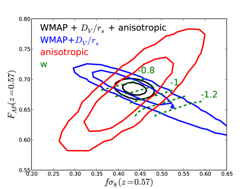
Figure 10: Constraints from Reid et al. (2012) on the anisotropic galaxy clustering parameters $f\sigma_{8}$ and $F_{AP}$ at $z=0.57$ are shown in red. The blue contour projects the combined constraints from WMAP and the spherically-averaged BAO position from BOSS, $D_{V}/r_{s}$ at $z=0.57$; dashed green lines indicate the mean value of $w$ in the region allowed by WMAP$+D_{V}/r_{s}$; the black contour combines the anistropic measurement with the CMB and spherically-averaged BOSS BAO position, resulting in a factor of $\sim 4$ improvement in the constraint on $w$.

Cosmological model	Data set	$\Omega_{\rm m}$	1000$\Omega_{\rm k}$	$H_{0}$	$w_{0}$	$w_{a}$
$\Lambda$CDM	CMB + CMASS + SNeIa	0.285 $\pm$ 0.014	0	68.9 $\pm$ 1.1	-1	0
$\Lambda$CDM	CMB + CMASS	0.291 $\pm$ 0.014	0	68.5 $\pm$ 1.2	-1	0
$\Lambda$CDM	CMB + CMASS + $H_{0}$	0.281 $\pm$ 0.013	0	69.5 $\pm$ 1.1	-1	0
O$\Lambda$CDM	CMB + CMASS + SNeIa	0.281 $\pm$ 0.014	-9.2 $\pm$ 5.0	67.7 $\pm$ 1.3	-1	0
O$\Lambda$CDM	CMB + CMASS	0.288 $\pm$ 0.017	-8.5 $\pm$ -5.4	67.4 $\pm$ 1.3	-1	0
O$\Lambda$CDM	CMB + CMASS + $H_{0}$	0.277 $\pm$ 0.014	-6.0 $\pm$ 4.9	68.8 $\pm$ 1.3	-1	0
wCDM	CMB + CMASS + SNeIa	0.292 $\pm$ 0.015	0	68.0 $\pm$ 1.4	-0.94 $\pm$ 0.05	0
wCDM	CMB + CMASS	0.313 $\pm$ 0.017	0	65.9 $\pm$ 1.5	-0.87 $\pm$ 0.05	0
wCDM	CMB + CMASS + $H_{0}$	0.291 $\pm$ 0.015	0	68.2 $\pm$ 1.4	-0.93 $\pm$ 0.05	0
OwCDM	CMB + CMASS + SNeIa	0.285 $\pm$ 0.017	-8.2 $\pm$ 5.5	67.4 $\pm$ 1.5	-0.98 $\pm$ 0.05	0
OwCDM	CMB + CMASS	0.307 $\pm$ 0.022	-3.9 $\pm$ 6.8	65.9 $\pm$ 1.6	-0.90 $\pm$ 0.07	0
OwCDM	CMB + CMASS + $H_{0}$	0.285 $\pm$ 0.018	-3.7 $\pm$ 5.7	68.2 $\pm$ 1.5	-0.95 $\pm$ 0.07	0
$w_{0}w_{\rm a}$CDM	CMB + CMASS + SNeIa	0.280 $\pm$ 0.018	0	68.8 $\pm$ 1.6	-1.13 $\pm$ 0.12	0.65 $\pm$ 0.36
$w_{0}w_{\rm a}$CDM	CMB + CMASS	0.313 $\pm$ 0.037	0	66.2 $\pm$ 2.8	-0.86 $\pm$ 0.34	-0.14 $\pm$ 1.04
$w_{0}w_{\rm a}$CDM	CMB + CMASS + $H_{0}$	0.261 $\pm$ 0.037	0	71.2 $\pm$ 2.3	-1.29 $\pm$ 0.19	1.02 $\pm$ 0.48

Table 5: Estimates of basic cosmological parameters for different models and combinations of data sets.

When we assume a cosmological constant and fix the spatial curvature to zero ($\Lambda$CDM), we obtain a 5 per cent constraint on $\Omega_{\rm m}$ and a 2 per cent constraint on Hubble constant from the joint fit to CMB data, CMASS geometric measurements and SNeIa data. When the values of $w_{\rm a}$ and $\Omega_{\rm k}$ are fixed to zero, $w_{0}$ can be measured with a precision of 5 per cent.

These results are consistent with the results reported in Anderson et al. (2012) who use only the position of the BAO peak and Sanchez et al. (2012) who use the full shape of the monopole. Our measurements are derived from the same sample but use additional information from the shape and the amplitude of the quadrupole. This allows us to get significantly stronger constraints with the CMASS data only (see Fig. 8). When CMASS data is combined with other data sets this improvement is somewhat mitigated but still present. When combined with CMB data and for the $\Lambda$CDM model our measurements improve constraints on $\Omega_{\rm m}$ by about 18 per cent relative to the BAO only results reported in Anderson et al. (2012). The central values are consistent within $1\sigma$. The biggest improvement is on the DE parameter $w_{0}$ ($-0.87\pm-0.05$ compared with $-0.87\pm 0.24$ in wCDM model), where we find a factor of four improvement over BAO only results even after combining the BAO measurements with WMAP7. Fig. 10 illustrates why including the information from anisotropic BOSS clustering improves the constraint on $w$ so much, even though Fig. 4 shows that the marginalized one-dimensional constraints on $f\sigma_{8}$ and the Alcock-Paczynski parameter $F$ are individually not very constraining on $w$. The anisotropic BOSS constraint (red) is nearly perfectly perpendicular to the degeneracy direction opened by $w$ in the $f\sigma_{8}(z=0.57)-F_{AP}(z=0.57)$ plane for the data combination of WMAP7 with the BOSS measurement of $D_{V}(z=0.57)/r_{s}$. When combined with CMB data our measurements of growth and geometry prefer $w_{0}>-1$ at about $2\sigma$ confidence level. When SNeIa or $H_{0}$ data is added the agreement with $\Lambda$CDM becomes better.

5.3 Constraining the effective potential of scalar-field dark energy

We also constrain parameters of scalar field dark energy models, as described in Section 4.3, for spatially-flat cosmological models.

Fig. 11 shows constraints on the parameter $\alpha$ describing the potential of the slowly rolling scalar field and parameters $M$ and $f$ describing the potential of PNGB field from our geometric and growth measurements combined with WMAP 7 shape and amplitude prior. For both models we assume a spatially-flat Universe. We also assume a uniform theoretical prior $0<f/\sqrt{M_{\rm pl}}<1$ and $M/\sqrt{M_{\rm pl}H_{0}}$, where $M_{\rm pl}$ is the Planck mass.

The resulting constraints on basic scalar field parameters are presented in Table 6. In both cases the $\Lambda$CDM limit of the scalar field theories provides a good fit to the data. The $\alpha$ parameter is constrained to be less than 0.48 at $1\sigma$ confidence level, which is slightly better compared to the previously reported best constraint (Samushia, 2009). $M$ is needs to be at least 88 per cent of the Planck mass. For comparison previous studies used SNeIa data to constrain $M$ to be more than third of the Plank mass (Dutta & Sorbo, 2008). The $\Lambda$CDM limits of PNGB model ($\phi_{0}/f=0.0$) and power-law model ($\alpha=0$) provide a good fit to data.

Figure 11: Confidence levels ($1\sigma$ and $2\sigma$) for joint fits to parameters $\Omega_{m}$ and $\alpha$ for the inverse-power law model (left panel) and parameters $M$ and $f$ for the PNGB model (right panel) adopting the CMASS DR9 measurements of $D_{\rm V}$ and $F$ and the WMAP7 shape prior. On the right panel, the shaded area corresponds to the region allowed at $2\sigma$. Without adding the growth rate information the PNGB constraints are weak. The dotted line shows $1\sigma$ contour from geometric measurements only, almost all of the remaining phase space is allowed at $2\sigma$.

parameter	most likely value	$1\sigma$ confidence level
$\alpha$	$0.16$	$<0.48$
$M/\sqrt{M_{\rm pl}H_{0}}$	$1.0$	$>0.9$
$\phi_{0}/f$	$0.11$	$<1.17$

Table 6: Most likely values and $1\sigma$ confidence level constraints on parameters describing scalar field dark energy from our geometric and growth measurements and CMB shape and distance prior.

5.4 Constraining model-independent properties of DE

To reconstruct the model-independent properties of the late-time Universe, as described in Section 4.4 we will use the geometric Reid et al. (2012) measurements in combination with the previous AP constraints presented in Table 3. These estimates were derived using different fitting methods, measurements and range of scales. We ignore these differences in our analysis and will treat the reported measured values and their errorbars as Bayesian likelihoods of $D_{\rm V}$ and $F$ at the redshifts of interest.

If we assume that the Universe is well described by a FRW metric, the Hubble rate and expansion rate and the relationship with distances can be written without a reference to a particular DE model; they can be expressed purely as functions of $\dot{a(z)}$ through

$$D_{A}(z)=\frac{c}{(1+z)}\displaystyle\int_{0}^{z}\frac{dz^{\prime}}{\dot{a}(z^{\prime})(1+z^{\prime})},$$ (22)

$$H(z)=\dot{a}(z)(1+z).$$ (23)

where the scale factor $a$ is normalised such that $a=1$ today and dot denotes a time derivative.

Different methods for the model-independent reconstruction of the expansion history and properties of DE have been proposed in the past (see e.g., Alam, Sahni & Starobinsky, 2007; Turner & Huterer, 2007; Daly & Djorgovski, 2007; Shafieloo & Clarkson, 2010; Crittenden et al., 2012, and references therein). The most popular approach is to parametrize the dimensionless coordinate distance in the integral in Eq. (22) by a polynomial and express the scale factor through its first and second derivatives. Blake et al. (2011c) used the method of Shafieloo et al. (2006) to reconstruct the comoving distance from SNeIa data, which, combined with their measurements of $F$, enabled an estimate of $H(z)$.

We will adopt an alternate approach that does not require taking derivatives of the quantities reconstructed from data, which has been shown to introduce artificial oscillations in reconstructed variables (Lazkoz, Salzano & Sendra, 2012). We assume that $a^{3}H^{2}(a)=a\dot{a}^{2}\equiv y(a)$ is a smooth function of the scale factor, so that it can be approximated by a third order polynomial. We have checked that this approximation holds to a percent level for all conventional DE models for wide range of redshifts; for $\Lambda$CDM this expansion is exact up to the radiation dominated era. Eqs. (23) can be rewritten in terms of $y(a)$ as

$$D_{A}(a)=ca\displaystyle\int_{a}^{1}\frac{a^{\prime 3/2}da^{\prime}}{\sqrt{y(a^{\prime})}},$$ (24)

$$H(a)=\sqrt{\frac{y(a)}{a^{3}}}.$$ (25)

We map $y(a)=\displaystyle\sum_{i=0}^{3}y_{i}a^{i}$ into $D_{\rm V}$ and $F$ using Eqs (24) – (25) and compare the results to geometric measurements. We compute a likelihood of polynomial coefficients of the expansion of $\mathcal{L}(a_{i})$ and map it onto the likelihood of deceleration parameter $q(z)$ which is defined in Eq. (19) by

$$\mathcal{L}^{\rm q}(q)=\mathcal{L}(y[a_{i}]).$$ (26)

The left panel of Fig. 12 presents the results of the reconstruction of $q(z)$ using our geometric measurements from the CMASS DR9 data combined with previous similar geometric measurements from 6dFGRS, SDSS-II and WiggleZ surveys. The reconstruction uses only the geometric measurements, shape prior from WMAP7 data and theoretical priors of spatially-flat FRW metric and smoothness of $a^{3}H^{2}(a)$. The recovered deceleration parameter is less than zero at redshifts $z<0.3$ and more than $3\sigma$ from $q=0.5$ as predicted by EdS model. Lampeitl et al. (2010) were able to derive a much stronger constraint of $q=-0.34\pm 0.18$ using SNeIa data only, however they had to assume constant $q$ while we allow $q$ to have non-zero higher derivatives.

Figure 12: Confidence levels ($1\sigma$ and $2\sigma$) for the deceleration parameter as a function of redshift and ${\rm Om}(z)$ reconstructed from the compilation of geometric measurements in tables 2 and 3. $H_{0}$ is marginalised over with an HST prior. The dotted line in the left panel demarcates accelerating expansion (below the line) from decelerated expansion (above the line). The dashed line in both panels shows the expectation for an EdS model.

The right panel of Fig. 12 presents a similar reconstruction of ${\rm Om}(z)$ parameter. The reconstructed ${\rm Om}(z)$ is consistent with being constant and is more than $5\sigma$ from the EdS predicted value of ${\rm Om}(z)\equiv 1$. Our reconstructed $q(z)$ and ${\rm Om}(z)$ are consistent with those reconstructed by Blake et al. (2011c); our results are smoother as a function of redshift because of the different reconstruction method used.

Our geometric measurements can be used to derive an estimate of Hubble expansion rate at $z=0.57$, since

$$H(z)=c\frac{(zF^{2})^{1/3}}{D_{\rm V}}.$$ (27)

This measurement of $H(z)$ combined with an independent measurement of $H_{0}$ can be used to estimate the increase in the fractional energy density of DE with respect to nonrelativistic matter from $z=0.57$ to present day. If we assume a flat FRW background and two dominant components $\Omega_{\rm m}$ and $\Omega_{\rm DE}$ then

$$\frac{\rho_{\rm DE}(z)}{\rho_{\rm m}(z)}=\frac{H(z)^{2}/H_{0}^{2}-\Omega_{\rm m}(1+z)^{3}}{\Omega_{\rm m}(1+z)^{3}}.$$ (28)

Combining our estimate of $H(z=0.57)$ with the Riess et al. (2011) measurement of $H_{0}$ and a WMAP 7 prior of $\Omega_{\rm m}h^{2}=0.1334\pm 0.0056$ we find $\rho_{\rm DE}(z=0)/{\rho_{\rm m}(z=0)}=3.09\pm 0.32$ and $\rho_{\rm DE}(z=0.57)/{\rho_{\rm m}(z=0.57)}=0.67\pm 0.13$. This means that the fractional contribution of DE to the total has increased by a factor of $\sim 4.7$ since $z=0.57$, lending support to the notion that expansion dominated by DE is a relatively recent occurrence.

5.5 Is there an evidence for deviations from flat LCDMGR?

As discussed in Reid et al. (2012) the observed galaxy clustering when combined with CMB data is fully consistent with LCDMGR expectations. Nevertheless, several of our fits to one-parameter extensions of flat LCDMGR ($\gamma$, $\mu_{1}$, and $w_{0}$) indicate a $\sim 2\sigma$ preference for values away from the fiducial. The data, however, demand these extra parameters at a much lower significance than $2\sigma$: the difference in the best fit $\chi^{2}$ values between flat LCDMGR and these one-parameter model extensions is only $\sim$2.5. A similar effect has been observed for the effective number of Neutrinos ($N_{\rm eff}=3$ in the standard model of particle physics), where the Bayesian posterior likelihood resulting from the CMB data has been shown to prefer $N_{\rm eff}>3$ at high confidence level. The Gonzalez-Morales et al. (2011), however, showed that in this case the priors imposed on cosmological parameters have a strong effect on the posterior likelihood of $N_{\rm eff}$ and after removing this prior-dependency the preference for the deviation from $N_{\rm eff}=3$ is much lower.

6 Conclusions

We have used the Reid et al. (2012) measurements of angular distance, Hubble expansion rate and growth rate derived from the anisotropic clustering of BOSS CMASS DR9 galaxies to place constraints on deviations from the standard cosmological model that assumes a $\Lambda$CDM background with structure formation driven by GR. The geometric measurements of $D_{\rm V}$ and $F$ are complementary to similar measurements from the BAO peak position (Anderson et al., 2012) and the full shape of the correlation function (Sanchez et al., 2012) and strengthen existing constraints on parameters describing the time-dependence of DE energy density. The RSD measurement of $f\sigma_{8}$ was shown to provide an additional constraint on the parameters describing deviations from GR and helped to significantly tighten DE constraints derived from geometric measurements. We now highlight our findings by using them to answer fundamental questions about our Universe.

How much do RSD measurements enhance the geometric measurements?
When GR is assumed the RSD measurements of growth break parameter degeneracies present when using purely geometric measurements, and consequently significantly tighten constraints on basic cosmological parameters. The addition of growth rate information improves constraints on $\Omega_{\rm m}$ by 18 per cent relative to the case where only BAO peak position data is used. The improvement is most dramatic for the $w_{0}$ parameter constraints, which improve by a factor of four compared to BAO only results (see Table 5).

Does GR provide a good description of data?
When $\Lambda$CDM is assumed our measurements of growth and geometry show a $2\sigma$ preference for models in which the growth of structure is weaker compared to GR. Adding previous RSD measurements at other redshifts brings the best-fit closer to GR value but still prefers somewhat weaker growth. This results from the fact that most RSD measurements of $f(z)\sigma_{8}(z)$ with high signal-to-noise are below GR predictions (see Fig. 1).

Does the Cosmological Constant provide a good description of data?
Assuming GR, our measurements of growth and geometry show a $2\sigma$ preference for $w>-1$. When combined with SNeIa data, the best-fit is closer to the cosmological constant model and the discrepancy is lowered to about $1\sigma$. It should be noted that, for DE as well as GR, the $2\sigma$ preference means a preference in terms of relative Bayesian likelihood.

How well can the DE scalar field potential be constrained?
We demonstrated that our measurements of growth and geometry, when combined with CMB information, provide strong constraints on scalar field DE model parameters. The constraints obtained are better than previously reported from different combinations of data sets. The flat potential (Cosmological Constant) provides a good fit to data.

Has the expansion of the Universe accelerated recently?
We employed a model-independent approach that relies on very few general assumptions to reconstruct the “deceleration parameter” at low redshifts. We showed that current AP measurements provide $2$ to $3\sigma$ evidence for the accelerated Universe at low redshifts. Much stronger measurements of $q(z)$ exist in the literature, but they depend on additional assumptions about the nature of DE.

Did DE emerge as a dominant component only very recently?
Our estimate of $H(z=0.57)$ combined with an estimate of $H_{0}$ suggest that energy density of DE relative to nonrelativistic matter was about 4.5 times lower at $z=0.57$.

Is the standard $\Lambda$CDMGR model still valid?
Measurements of growth and geometry from CMASS DR9 sample allow for a very strong test of MG and DE. When combined with WMAP7 data they show a $2\sigma$ preference for either weaker gravity or $w>-1$. However, in terms of absolute $\chi^{2}/{\rm dof}$, the simple $\Lambda$CDMGR model still provides a good fit to the data.

Appendix A NonGaussianity in posterior likelihood

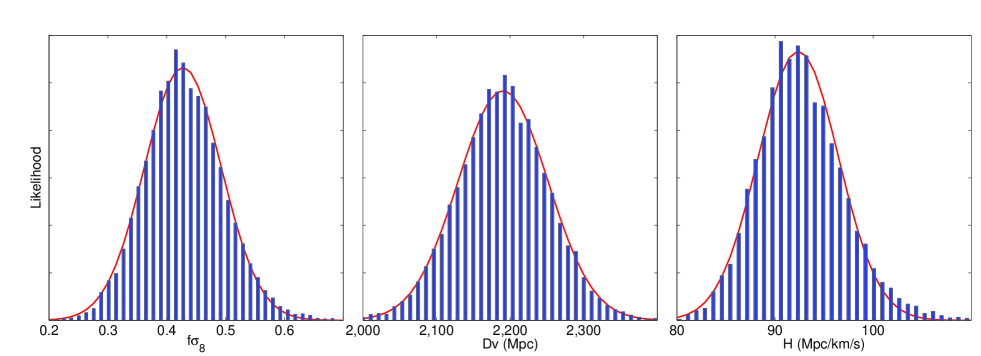
Figure 13: Marginalized one-dimensional posterior likelihood of parameter $f\sigma_{8}$, $D_{A}$ and $H$ from Reid et al. (2012) used in our analysis (The likelihood is in arbitrary units). The bars show the real distribution, while the solid line represents the Gaussian approximation that we use.

Figure 13 shows the marginalized one-dimensional posterior likelihood of parameters $f\sigma_{8}$, $D_{A}$ and $H$ used in our analysis. Our multivariate Gaussian approximation to the likelihood works very well everywhere except for the tails of the likelihood where it deviates from the empirical likelihood by not accounting from for small positive skewness in $f\sigma_{8}$ and $H$. We have checked that the derived likelihood of modified gravity and dark energy parameters does not change at 1 and 2$\sigma$ confidence levels when the Gaussian approximation is used instead of the whole likelihood.

References

- Amblard, Vale & White (2004) Amblard A., Vale C., White M., 2004, New Astron., 9, 687
- Amendola, Kunz & Sapone (2008) Amendola L., Kunz M., Sapone D., 2008, Cosmology Astropart. Phys., 4, 13
- Amin, Wagoner & Blandford (2008) Amin M.A., Wagoner R.V., Blandford R.D., 2008, MNRAS, 390, 131
- Anderson et al. (2012) Anderson L., et al., 2012, preprint, [arxiv:1203.6594]
- Alam, Sahni & Starobinsky (2007) Alam V., Sahni A., Starobinsky A., 2007, JCAP, 11, 0702
- Albrecht et al. (2009) Albrecht A., et al., 2009, “Findings of the Joint Dark Energy Mission Figure of Merit Science Working Group”, [arxiv:0901.0721]
- Alcock & Paczynski (1979) Alcock C., Paczynski B., 1979, Nature, 281, 358.
- da Angela et al. (2008) da Angela J., et al., 2008, MNRAS, 383, 565
- Appleby & Linder (2012) Appleby S.A., Linder E.V., 2012, JCAP, 08, 026
- Bertschinger (2006) Bertschinger E., 2006, ApJ, 648, 797
- Beutler et al. (2011) Beutler F., et al., 2011, MNRAS, 416, 3017
- Beutler et al. (2012) Beutler F., et al., 2012, MNRAS, 423, 3430
- Blake et al. (2011a) Blake, et al., 2011a, MNRAS, 415, 2876
- Blake et al. (2011b) Blake, et al., 2011b, MNRAS, 418, 1707
- Blake et al. (2011c) Blake C., et al., 2011c, MNRAS, 418, 1725
- Blake et al. (2012) Blake C., et al., 2012, MNRAS, 425, 405
- Bloomfield & Flanagan (2012) Bloomfield J.K., Flanagan E.E., 2012, JCAP, 10, 039
- Buchdahl (1970) Buchdahl H.A., 1970, MNRAS, 150, 1
- Cabre & Gaztanaga (2009) Cabre A., Gaztanaga E., 2009, MNRAS, 393, 1183
- Caldwell, Cooray & Melchiorri (2007) Caldwell R., Cooray A., Melchiorri A., 2007, PRD, 76, 023507