A flavor model in RS1
Abstract
Randall Sundrum models provide a possible explanation of (gauge-gravity) hierarchy, whereas discrete symmetry flavor groups yield a possible description of the texture of Standard Model fermion masses. We use both these ingredients to propose a five-dimensional extension of the Standard Model where the mass hierarchy of the four-dimensional effective field theory is obtained only using localizations parameters of order 1. We consider a bulk custodial gauge symmetry group together with an Abelian group: the model turns out to yield a rather minimal extension of the SM as it only requires two brane Higgs fields to provide the desired Yukawa interactions and the required spontaneous symmetry breaking pattern. In fact, the presence of an extra-dimension allows the use of the Scherk-Schwarz mechanism to contribute to the breaking of the bulk custodial group down to the SM gauge symmetry. Moreover, no right-handed neutrinos are present and neutrino masses are generated radiatively with the help of a bulk charged scalar field that provides the Lepton-number violation. Using experimental inputs from the Global Neutrino Analysis and recent Daya Bay results, a numerical analysis is performed and allowed parameter regions are displayed.
pacs:
11.30.Hv, 12.15.Ff, 14.60.PqI Introduction
The Standard Model (SM) gauge group is a priori consistent with a large flavor group that is not observed experimentally and Yukawa couplings and mixings are introduced to comply with such experimental evidence Cabibbo:1963yz . However, the pattern of fermion masses and mixing angles and the nature of the neutrino mass (whether Dirac or Majorana) is not constrained by the gauge symmetry and it is thus natural to go beyond the SM to seek for a theoretical explanation of the observed masses and angles and of their hierarchies. To date a promising direction towards the understanding of flavor physics in the SM – notably of fermion mass matrices and mixing – has been the study of particular textures (in the quark sector), such as the Nearest Neighbor Interactions (NNI) texture Branco:2010tx ; Harayama:1996am ; NNI and the Fritzsch type textures Fritzsch:1977vd , and the introduction of flavor symmetry groups that constrain the structure of the fermion mass matrix to reproduce the desired texture. The mixing in the lepton sector has also given strong support to the idea of an underlying flavor symmetry and many flavor symmetry groups have been proposed so far Altarelli:2010gt ; Ishimori:2010au ; Altarelli:2010fk ; of them discrete groups have proved to be quite successful and we keep exploring such direction in the present work.
Although the aforementioned approach, involving (discrete) flavor groups, provides a possible description of the pattern of fermion masses and mixing angles, it seems not to be able to explain the hierarchy(ies) among the different species of fermionic masses. i.e., the flavor symmetry explains the number and location of the ”zeros” in the textures for the fermion mass matrices, but not the relative size among the non-zero entries. In other words it appears that, in order to obtain experimentally suitable values for such physical quantities, one needs to allow for parameters of quite different order of magnitude. Such hierarchy problems have proved to be quite hard, in the framework of four-dimensional non-supersymmetric theories. On the other hand in the context of extra-dimensions, several models – with flat or warped extra-dimensions – were proposed as solutions to hierarchy problems, mostly focusing on the gauge-gravity hierarchy. In particular the Randall-Sundrum model 1 (RS1) Randall:1999ee has drawn a great deal of attention as it provides a possible description of the TeV-Planck hierarchy with a small (Planck size) extra-dimension and treats the TeV scale as a derived scale. The geometry of such space is a slice of five-dimensional Anti-de Sitter space, a warped product between four-dimensional space, and an extra dimension with the topology of an interval whose extrema are the fixed points of a orbifold symmetry. The space thus ”ends” on two flat four-dimensional planes (branes) located at the extrema of the extra dimension. Extra-dimensional models, especially Randall-Sundrum models, have also been explored in the context of the SM physics as fermion masses might be explained in terms of the overlaps between the extra-dimensional profiles of fermions and Higgs(es) Grossman:1999ra ; ArkaniHamed:1999dc ; Gherghetta:2000qt ; Huber:2000ie ; Huber:2003tu .
It is then interesting to consider the possibility of merging both scenarios – flavor symmetries and hierarchy from extra dimensional settings – in a single setup and to determine if a viable model can be constructed. This work presents one such case. To do this we use a minimally-extended version of the SM that incorporates a discrete flavor group, and that reproduces fermion mass patterns as well as mixing angles in both the quark and lepton sectors. The model is minimal in the sense that it contains the SM matter fields only (in particular, it does not add right-handed neutrinos), an extended Higgs sector composed of two Higgs SU(2) doublets, a Lepton number violating scalar, and the smallest Abelian group that renders the NNI textures for the quark mass matrices, namely the cyclic group .
The model is detailed in the forthcoming section, however let us stress here that such approach was already taken by other groups. For example, in Chen:2008qg , a realization of the so-called Lepton Minimal Flavor Violation scenario was obtained in the framework of RS with right-handed neutrinos. There it was found that the first Kaluza-Klein (KK) mass scale could be as low as TeV. Along similar lines, but for the quark sector and providing a solution to the issue of flavor changing neutral currents in extra dimensional settings, the work in Bauer:2011ah extends the strong sector in the bulk with an additional SU(3), broken down to Quantum Chromodynamics (QCD) by boundary conditions that render the model safe, even for a KK scale of TeV. Closer to our approach is the work by Kadosh and Pallante Kadosh:2010rm , where an flavor symmetry is introduced in a RS setup. The main difference with our model is that, unlike Kadosh:2010rm , we use a flavor group that reproduces the mixing matrices in both the quark and lepton sectors automatically, without the need of introducing additional flavon fields to generate non-zero entries and/or further suppressions. This makes our model more economical in terms of additional fields and more tractable, specially in the scalar sector. Another important difference is that in our model neutrino masses are generated radiatively and there is no need to introduce right-handed neutrinos, as mentioned above.
The gauge and Yukawa sectors of our model are presented in section II, where the expressions for the mass matrices in both the lepton and quark sectors are described and explicitly shown. Section III shows the numerical analysis and results for both sectors and some remarks about the scalar potential and flavor changing neutral currents. Finally we present the conclusions. An appendix has been included in order to maintain the discussion in the paper self contained.
II Model
The five-dimensional field theory we consider is a higher-dimensional extension of the SM and lives in the RS1 background. Such space is a slice of AdS5 space of Planck-size curvature, where the fifth dimension is taken to be an orbifolded circle of radius , and fields are odd or even under the action of the orbifold, i.e. under reflection . In other words the extra dimension has the topology of a line that stretches between and and the latter are fixed points of the orbifold, where two flat 3-branes, one with positive and the other with negative tension, are accommodated. The brane located at is referred to as the ”UV brane”, whereas the brane located at is referred to as the ”IR brane”. The bulk line element is thus given by
| (1) |
with being (proportional to) the AdS curvature, and the TeV-Planck hierarchy is realized provided . Such geometry is realized with a negative bulk cosmological constant and with the aforementioned brane tensions: all three are of Planck size. Moreover, all the fields we deal with have vacuum expectation values (vevs) of order at most TeV, and we may thus neglect their backreaction to the geometry (1).
The five-dimensional model we consider has a gauge-symmetry group that includes the Standard Model custodial symmetry in order to suppress excessive contributions to the Peskin-Takeuchi parameter Peskin:1990zt ; Agashe:2003zs , augmented with a discrete Abelian group , hence . All the fields of our model are charged under and, with the exception of the Higgs fields, are all bulk fields, along the lines of what is done in Agashe:2003zs . This setup thus enjoys a very nice interpretation in terms of AdS/CFT correspondence as only the Higgs fields are seen as TeV-scale composites of the strongly-coupled sector of the four-dimensional theory and, since all other fields are bulk fields, all the phenomenology of the model is addressable from the weakly-coupled five-dimensional model.
The matter content of the model involves (three families of) left-handed quark doublets and lepton doublets along with two copies of right-handed quark doublets, and , and one copy of right-handed lepton doublets, ; the zero-modes of ”tilded” fields will be projected out from the IR brane by Scherk-Schwarz gauge-symmetry breaking Agashe:2003zs and only their KK modes are eventually non-zero on the brane. We then use two Higgs fields and that are bi-doublets of and are confined to the IR brane. Lastly, we introduce a bulk singlet scalar field charged under hypercharge and lepton number that participates in neutrino mass generation. The charge assignment for all such fields is similar to the one given in Aranda:2011rt , namely
| (2) | |||||
| (3) |
for the quark sector, with , and ,
| (4) | |||||
| (5) |
for the lepton sector, with and , and
| (6) |
for the scalars with , and . The main difference with Aranda:2011rt is that the left-handed up-type and down-type quarks have the same charges; the reason is dictated by the fact that we are using Higgs bi-doublets confined on the IR brane. These fields transform as under gauge transformations (, where are the Pauli matrices) and, as explained later, are responsible for the spontaneous breaking of on the IR brane. In other words the vevs of are singlets
| (7) |
so that ¿, with , and and thus enter on equal footing in the Yukawa lagrangian and must then have the same charges.
It is easy to check that (7) is invariant under the diagonal part of , namely
| (8) |
and thus preserves .
II.1 Gauge-symmetry breaking
The bulk (custodial) gauge symmetry must be broken down to the SM gauge group on the four-dimensional effective action at TeV scale and usual electroweak spontaneous symmetry breaking must also be accounted for. We realize this in the same way as in Agashe:2003zs ; Kadosh:2010rm by orbifold Scherk-Schwarz projection, i.e. by assigning independent orbifold charges to a field at the two different ends of the interval, and with canonical spontaneous breaking.
We can impose on the bulk fields a charge assignment. For scalar fields this corresponds to the field transformations
| (9) | |||||
| (10) |
with and being the fixed points of . For 5D spinors, single valuedness of the lagrangian upon the action of requires
| (11) |
We can fix and decompose the 5D 4-spinor as with being left-handed (right-handed) Weyl spinors, in the 4D sense. At the fixed points, i.e. setting in (11), we thus have that the left-handed Weyl spinor has charges and the corresponding right-handed Weyl spinor has charges 666Henceforth, when referring to the fermionic charges, we will indicate the charges associated to the left-handed part of the doublet.. Below we mostly only care about the extra-dimensional zero-modes, whose profiles are summarized in Appendix A. We thus have that the fermion left-handed zero mode (100) only exists for charges whereas the right-handed zero mode exists for . In other words, other non-trivial orbifold projections lift the mass of the zero-mode. For vector fields, whose would-be zero-modes are constant, we again have that only allows for massless zero modes and other charge assignments lift the mass and thus realize the low-energy symmetry breaking.
In our model we break gauge symmetry down to on the UV brane via Scherk-Schwarz mechanism, i.e. we assign to the electrically charged vector bosons of , and to the neutral gauge boson. Since the former couple the upper and lower parts of the right-handed fermion doublets, single-valuedness of the bulk lagrangian requires that if the upper part is even, on the UV brane, the lower part must be odd and viceversa. Hence, in order to have zero-modes for both the upper and lower parts of the right-handed quarks, we need to double the number of right-handed fields Agashe:2003zs in the quark sector, as already mentioned above. The charge assignment for such fields thus reads
| (12) |
for the quark sector, and
| (13) |
for the leptonic sector. A vev on the UV brane then provides the breaking Agashe:2003zs .
On the IR brane the vevs of the Higgs bi-doublets provide the spontaneous breaking . Hence finally the superposition of all such breakings only leaves untouched. In fact
| (14) |
with being the generators of (above the tensor product is left implied.)
II.2 Yukawa Sector
II.2.1 Quarks
The mass terms for the quarks come from the following Yukawa interactions on the IR brane
| (15) | |||||
where is the Planck-scale and are dimensionless parameters assumed of that, together with the quark extradimensional profiles, generate the effective four-dimensional Yukawa couplings. The charge assignments for the quark and scalar fields then induce the desired Yukawa NNI textures (writing separately each scalar contribution)
| (22) |
which after electroweak symmetry breaking lead to the following quark mass matrices
| (23) |
with denoting the vevs. The are the effective four-dimensional Yukawa couplings that depend on the fermion extradimensional profiles overlap with the Higgs bi-doublets at the IR boundary. Thus, under the zero mode approximation (ZMA) (see Appendix for the KK decomposition and the explicit fermion profiles), each of the Yukawa terms above looks like
where , , and , are family indices accordingly chosen (note also the inclusion of a canonically-normalizing factor for the Higgs bi-doublet). The effective Yukawa coupling, given by the product inside the curly brackets, depends on two quark localization – parameters
| (25) |
where since the left handed components of the and quarks form an doublet. In order to extract the – parameters that lead to experimentally allowed observables, we follow the Harayama parametrization in reference Harayama:1996am , which is a transformation of the up – and down – type quark mass matrices to a basis such that these display the NNI form without modifying the mass eigenvalues nor the CKM matrix entries. Once parametrized in that form and following Aranda:2011rt , we make the assumption that the and entries in are equal leading to
| (26) |
where are free parameters and
| (27) | |||||
| (28) | |||||
| (29) | |||||
| (30) |
with
| (31) |
are real matrices arising from the phase factorization of
| (32) |
with being diagonal phase matrices such that , and . Therefore, four parameters , and have to be chosen to fit the CKM matrix,
| (33) |
where diagonalize
| (34) |
We show the numerical results that reproduce the experimental values in section III.
II.2.2 Charged Leptons
The charged lepton masses are similarly obtained from the Yukawa interactions on the IR brane
| (35) |
After EWSB we obtain
| (36) |
The analog of Eq. (25) for charged leptons is
| (37) |
We can parametrize the matrix 777We do not assume as we did in the quark sector. following again Harayama:1996am , and so has dependence on both dimensionless parameters and
| (38) |
where and are the analogs of and for charged leptons and
| (39) |
Observe we can have two different solutions: the plus (minus) case is obtained taking the plus (minus) and minus (plus) signs in and respectively. Depending on which solution we choose we have two different regions for the mathematically allowed values of and , Region I (plus case) and II (minus case) respectively. Each region is constrained by the non – negative real values of an .
The matrix allows us to obtain the lepton – parameters by comparison to Eq. (36). Under the assumption that the phases in the charged lepton sector are zero, there are only two parameters left, and , whose actual values will be set by the neutrino sector results.
II.2.3 Neutrino sector
Since there are no right-handed neutrinos present in the model, neutrino masses are generated radiatively 888Using the well known dimension five Weinberg operator leads to unacceptable large values for the neutrino masses. This could be remedied by allowing unnatural small values of the dimensionless parameters, in contradiction to the philosophy of the general scenario. We therefore stick to the 4D renormalizable argument in Aranda:2011rt and consider the radiative mechanism. as in Aranda:2011rt . In the present extradimensional setting this mechanism is going to set two of the lepton -parameters. As can be noted in the next section, their values turn out to be , as any localization – parameter must be.
The radiative mechanism introduces a cubic Lepton number violating scalar interaction among the two SU(2)L doublets and the charged scalar , as well as the Zee operator coupling the left-handed lepton doublet to the singlet charged scalar Zee:1980 ; Babu:1988qv . The Randall-Sundrum geometry enhances this cubic scalar interaction as well as the Zee operator with factors proportional to the extradimensional profiles of the fermions and, if allowed to propagate through the bulk, those of the scalars. In the scenario where both scalar Higgs doublets are confined to the IR brane and the scalar singlet is a bulk field, the cubic scalar operator is an interaction on the TeV brane which looks like
| (40) |
where , are SU(2) indices and is antisymmetric and with mass dimension . Under the ZMA approach this term acquires the form
| (41) |
with the dimensionless antisymmetric coupling of (note also the inclusion of a canonically-normalizing factor for each one of the Higgs doublets). Thus, for an UV-peaked bulk field (whose approximated profile and normalization factor are shown in appendix A) the effective cubic operator acquires the form
| (42) |
where
| (43) |
has the correct mass dimension: and . An UV-peaked bulk (again in the ZMA) also modifies the Zee operator
| (44) |
(where and antisymmetric by the Pauli principle) and leaves it as
| (45) |
where is now dimensionless (and antisymmetric). The effective Zee operator then looks like
| (46) |
where is dimensionless and given by
| (47) |
Following the expressions in Aranda:2011rt for the 4D Majorana neutrino mass matrix and replacing the effective Yukawa and scalar couplings, we find that the Majorana neutrino mass matrix entries are
| (48) | |||||
| (49) | |||||
| (50) | |||||
| (51) | |||||
| (52) | |||||
| (53) | |||||
| (54) |
where (accounting for the scalar loop factor) is a function depending on the scalar masses of the charged Higgs, , and of the singlet scalar through
| (55) |
The parameters , , , and belong to the Yukawa matrix for charged leptons
and the entries , are those of the matrix .
Now, since and are antisymmetric we can rewrite the neutrino mass matrix entries as
| (56) | |||||
| (57) | |||||
| (58) | |||||
| (59) | |||||
| (60) | |||||
| (61) |
where is a common factor with dimension of inverse of mass
| (62) |
and
| (63) |
III Numerical Analysis
III.1 Lepton sector
To perform the numerical analysis in the lepton sector we used the experimental data at from the global neutrino data analysis in Schwetz:2011zk
| (64) |
with and normal (inverted) hierarchy and the recently Daya Bay results (confirmed at ) An:2012eh
| (65) |
which can be rewritten as
| (66) |
By convenience in the analysis we also define the following range for the neutrino squared mass differences ratio (at )
| (67) |
obtained by summing in quadrature the relative errors of and . The constraint over the sum of neutrino masses, eV presented recently in RiemerSorensen:2011fe is also considered.
The charged leptons masses used in the analysis are those given by the central values in PDG
| (68) | |||||
| (69) | |||||
| (70) |
As in reference Kadosh:2010rm we take the 5D scale to be where TeV is the reduced Planck mass, and the effective scale TeV generated by . For the other parameters involved in the neutrino mass sector we take TeV (recall this is the mass of the charged Higgses in the loop), , , and . Note that since is UV-peaked its mass is taken to its natural value of . We note however that the model can reproduce the neutrino sector even in the case of a very light -field (or even an IR-peaked field) due to the fact that only enters through the common factor in Eq. (62), and thus does not affect the diagonalization. Its only possible effect is in the absolute size of the neutrino mass matrix entries and it corresponds to acceptable changes of .
From the expressions for the neutrino mass matrix entries we observe that the only coefficients involved are and , and are taken to be and (this is only a choice and corresponds to similar values used in Kadosh:2010rm ). We also observe that all these parameters are contained in the factor, together with the parameter , and in consequence they do not affect the diagonalization matrix. Thus, the lepton mixing matrix defined by , where and are the diagonalization matrices in the charged lepton and neutrino sectors respectively, only depends on and the charged leptons mass matrix entries.
We use the standard parametrization of the given in PDG
| (71) |
where
| (72) |
with , and where is the Dirac-CP violating phase in the neutrino sector which we assume is zero. is a diagonal phase matrix containing the two Majorana CP violating phases.
The first step in our analysis consists of a scan over the mathematically allowed regions for the and parameters of the charged lepton mass matrix that lead to positive values for and in Eq. (II.2.2). The next step is to scan over values for values that lead to the allowed neutrino mass differences ratio and mixing angles. Finally, once the ranges for , and values that give the right angles and ratios are determined, we fit the values (or ) required to obtain the neutrino masses satisfying the constraint over the sum of neutrino masses RiemerSorensen:2011fe .
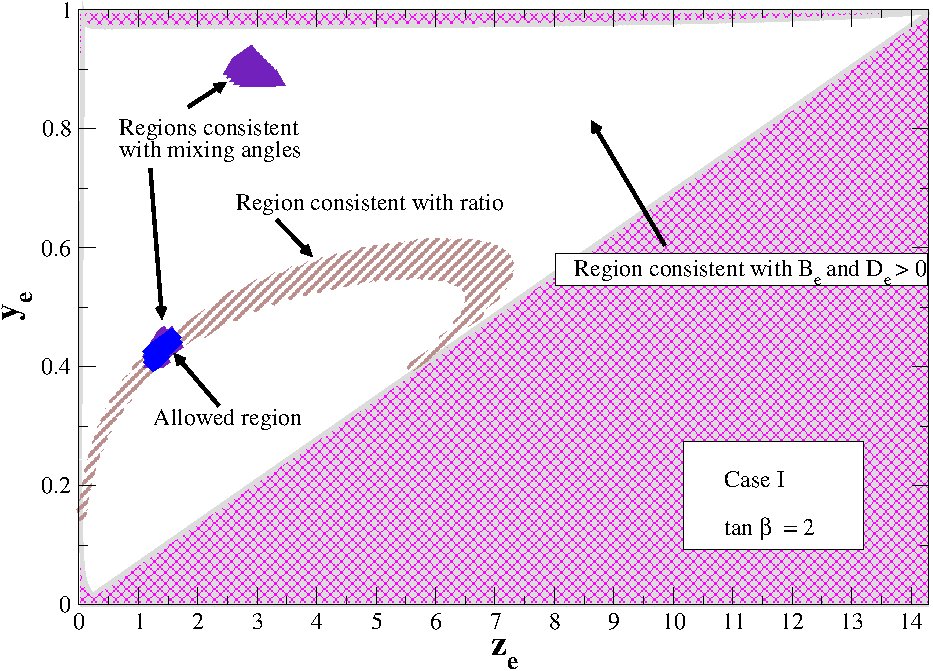
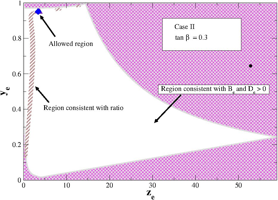
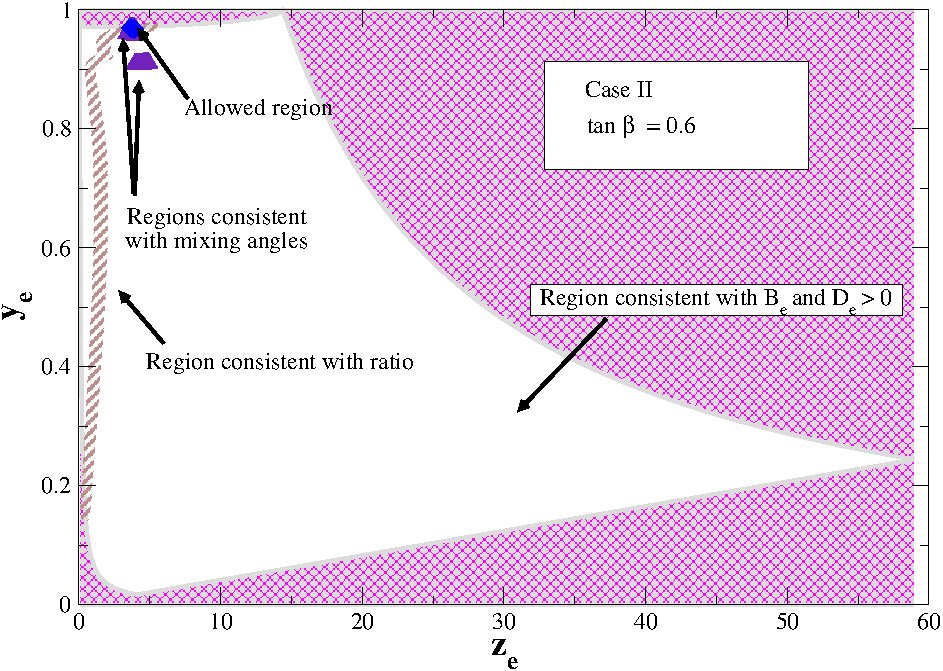
Performing the scan over values from to (in steps of ) and from to (in steps of ) we find that in Region I (plus case) the only value that works is while in Region II (minus case) and give acceptable values.
Figure 1 shows the parameter space obtained in this process. Note that in all cases there is a large region in the plane consistent with positive values for and . However the allowed region, consistent with all experimental information, is considerably reduced to small ranges in this parameter space. In the plots we label by allowed region the region of parameter space consistent with all experimental data, including the constraint on the sum of neutrino masses RiemerSorensen:2011fe .
We note that, as found in Aranda:2011rt , only inverted hierarchy for the neutrino masses is obtained in this model and that the resulting Majorana phases are found to be .
It is important to note that throughout the analysis all the have been taken to be of . In fact, except for and which are used in the fit and take values of in all cases, all other are set equal to . The same is true for all the profile – coefficients: all are of .
III.2 Quark sector
In Aranda:2011dx the values for the parameters , and leading to a correct CKM matrix were found to be , , and . The corresponding mass matrices (in TeV) read
| (76) | |||||
| (80) |
Comparing these matrices with Eq. (23) and using the values for found to work in the neutrino sector, we performed a fit to the – profile parameters and ’s. We find that it is possible to obtain solutions with all parameters of . In particular, for , experimental agreement is found for at least the following set of values , , , , , , and all other ’s equal to .
Thus, using dimensionless parameters of order one and dimensionful parameters associated to the scale of the setup, we find that it is possible to reproduce all observed masses and mixing angles in both the quark and lepton sector. Furthermore we accomplish this with a minimal set of additions and only left-handed neutrinos. It is important to recall that all results presented in this work have been obtained under the ZMA scheme and thus neglecting (although safely (Kadosh:2010rm, )) possible contributions from KK modes. Yet another possible source of contributions that must be investigated corresponds to contributions from higher order operators consistent with the gauge and flavor symmetries. In our case, the smallest higher order operators that could contribute are of the general form (and similarly for leptons). We find that the gauge and flavor invariant contributions, denoted by , to the zero entries in the mass matrices satisfy , where the denote the values of the non-zero entries. For the case , corresponding to contributions to the non-zero entries, we find . Thus, these contributions can be safely ignored.
Before concluding we make some remarks to be taken in full consideration in a future work. Our model has a potentially interesting scalar phenomenology that requires a complete study, including its vacuum stability and possible collider signals. Another important and related phenomenological issue is the presence of flavor changing neutral current (FCNC) effects. In our model there are two different possible contributions to FCNC that must be taken into consideration. The first one comes from the fact that we are dealing with a two (flavored) Higgs doublet model in which each Higgs couples to both the up and down quark sector. This can result in tree-level FCNC Atwood:1996vj ; Azatov:2009na that need to be analyzed and will induce constraints on the parameter space in the scalar potential. The second possibility is associated to the presence of mixing between the degrees of freedom of the effective 4D theory and their KK excitations. This is a problem that all extra dimensions models have to face. One has to guarantee that the corrections induced by this mixing will keep the agreement with observations forcing a lower bound, of order a few TeV, on the KK scale. In our model, the use of a custodial symmetry allows to consider a lower bound on the first KK mass to that imposed by electroweak precision measurements Agashe:2003zs (see also Chen:2008qg ; Bauer:2011ah ; Casagrande:2010si ). Furthermore if the flavor pattern of the Yukawa couplings holds in the 5D theory due to a flavor symmetry, an increased alignment between the 4D fermion mass matrix and the Yukawa and gauge couplings is obtained suppressing the amount of flavor violation induced by the interactions with KK states. Moreover, as pointed out in Kadosh:2010rm , a bulk flavor symmetry might also induce a cancellation of observable phases, therefore the dominant new physics contributions to the neutron and electron dipole moments and/or to will vanish.
IV Conclusions
A five-dimensional warped extension of the Standard Model is considered, where the space-time background is taken to be the Randall-Sundrum model 1, i.e. a warped extra-dimension of Planck size in an Anti-de Sitter bulk. We consider a Zero-Mode Approximation for the four-dimensional effective action one obtains as a dimensional reduction of the higher-dimensional theory and that, in the present case, constitutes an extension of the SM. In the model we study above almost all the fields in the 4D effective action are zero modes of bulk fields, in particular each left- respectively right-handed fermion mode has its five-dimensional counterpart; only the Higgs fields are purely four-dimensional and live on the IR brane (i.e. on the 4D plane located at the orbifold fixed point ) and, unlike the bulk fields, have no KK excitations. Bulk fermion fields come about with a (Planck size) mass term parametrized by a real number which determines the shape of the extra-dimensional profile of the field. The Yukawa interaction between Higgses and fermions is given in terms of overlapping integrals of zero-mode profiles for the fields involved and thus depends upon the aforementioned real parameters along with numerical coupling constant (hermitian) matrices ’s. In order to obtain a NNI-type quark mass matrix, we advocate the presence of a discrete symmetry upon which all fields are charged: the cyclic group is the smallest Abelian group consistent with the aforementioned texture. Also for the charged lepton sector the discrete symmetry fixes the form of mass matrix in a similar way as for the quark sector. For the quark sector (and similarly for the charged lepton sector) the numerical analysis goes as follows: first we consider the mass matrix parametrized à la Harayama in order for it to display NNI form. The diagonalization of the real squared counterpart of the previous mass matrix leaves four parameters that can be fixed using the experimental values for the CKM. In turn, this allows to fix the entries of the mass matrix itself and, by comparison of such entries with the ones foreseen by the overlaps of extra-dimensional profiles, one can obtain the compactification parameters ’s and the Yukawa dimensionless entries ´’s. All these parameters turn out to be of . For the charged leptons the parametrization goes slightly different and the (real) mass matrix depends upon two free parameters only constrained by the reality of the mass matrix: allowed parameter regions satisfying such constraints, as well as all experimental data, are graphically displayed. In the neutrino sector we choose not to introduce right-handed neutrinos in the model and generate neutrino masses radiatively. This is accomplished with the help of a bulk charged scalar field whose zero-mode is peaked on the UV brane (located at the fixed point ): such field also mediates the lepton number violation. With scalar field masses chosen to be TeV for the charged Higgses in the loops, and TeV, experimental data taken from global neutrino data analysis and Daya Bay results are matched by setting all parameters and parameters to values of . Although a complete phenomenological study of the model is under preparation, some comments regarding the scalar phenomenology of the model as well as its possible contributions to FCNC were also briefly discussed.
Acknowledgements.
OC is grateful to the University of Colima and the INFN Bologna for hospitality and support while parts of this work were completed. CA, AA, and ADR thank the Universidad Autónoma de Chiapas for its hospitality while part of this work was done. The work of OC was partly funded by SEP-PROMEP/103.5/11/6653. AA acknowledges support from CONACYT under the program Estancias de Consolidación, grant No. 145378.Appendix A On the zero mode profiles
We briefly review the computation of zero-mode profiles for some bulk fields, on the RS1 background considered above; we basically follow what is done in Pomarol00 ; Huber:2000ie . A bulk field satisfies a second order differential equation of the form
| (81) |
where , and ; note that compared to Pomarol00 ; Huber:2000ie ’s we redefined for the right-handed mode. Above and thus and . Upon Kaluza-Klein decomposition one gets
| (82) |
with and orthonormality conditions
| (83) |
so that
| (84) |
Here we only concentrate on the zero modes for which .
Vector field
For the vector field it is immediate to realize that the only possible zero-mode profile is constant and since the measure is also trivial in this case, we simply have .
Scalar field
For a bulk scalar field we have
| (85) |
that admits solutions
| (86) |
and the normalization factor is given by
| (89) |
where in the last expression we took into account that and , . Hence, including the measure factor the zero-mode profiles read
| (92) |
so that for the profile is peaked about the IR brane () and for the profile is peaked about the UV brane ().
Fermionic field
For a bulk fermionic field we follow Huber:2000ie with the aforementioned renaming of parameter for the right-handed mode. Hence
| (93) |
and
| (94) |
with
| (97) |
Hence, including the measure factor the zero-mode profiles read
| (100) |
so that for the profile is peaked about the IR brane () whereas for the profile is peaked about the UV brane ().
References
- (1) N. Cabibbo, Phys. Rev. Lett. 10, 531-533 (1963); M. Kobayashi, T. Maskawa, Prog. Theor. Phys. 49, 652-657 (1973).
- (2) G. C. Branco, D. Emmanuel-Costa, C. Simoes, “Nearest-Neighbour Interaction from an Abelian Symmetry and Deviations from Hermiticity,” Phys. Lett. B690, 62-67 (2010). [arXiv:1001.5065 [hep-ph]].
- (3) K. Harayama, N. Okamura, Phys. Lett. B387, 614-622 (1996). [hep-ph/9605215].
- (4) T. Ito, N. Okamura, M. Tanimoto, Phys. Rev. D58, 077301 (1998). [hep-ph/9711454]; T. Ito, M. Tanimoto, Phys. Rev. D55, 1509-1514 (1997). [hep-ph/9603393]; E. Takasugi, M. Yoshimura, Prog. Theor. Phys. 98, 1313-1323 (1997). [hep-ph/9709367]; Z. Berezhiani, A. Rossi, JHEP 9903, 002 (1999). [hep-ph/9811447]; G. C. Branco, M. N. Rebelo, J. I. Silva-Marcos, Phys. Lett. B597, 155-165 (2004). [hep-ph/0403016]; K. S. Babu, [arXiv:0910.2948 [hep-ph]]; G. C. Branco, L. Lavoura and F. Mota, Phys. Rev. D 39, 3443 (1989); G. C. Branco, D. Emmanuel-Costa, R. Gonzalez Felipe, H. Serodio, Phys. Lett. B670, 340-349 (2009). [arXiv:0711.1613 [hep-ph]]; G. C. Branco, D. Emmanuel-Costa and R. Gonzalez Felipe, Phys. Lett. B 477, 147 (2000) [arXiv:hep-ph/9911418]; H. Fritzsch, Z. -z. Xing, Y. -L. Zhou, Phys. Lett. B697, 357-363 (2011) [arXiv:1101.4272 [hep-ph]].
- (5) H. Fritzsch, Phys. Lett. B73, 317-322 (1978).
- (6) G. Altarelli, F. Feruglio, [arXiv:1002.0211 [hep-ph]].
- (7) H. Ishimori, T. Kobayashi, H. Ohki et al., Prog. Theor. Phys. Suppl. 183, 1-163 (2010). [arXiv:1003.3552 [hep-th]].
- (8) G. Altarelli, arXiv:1011.5342 [hep-ph].
- (9) L. Randall and R. Sundrum, Phys. Rev. Lett. 83, 3370 (1999) [hep-ph/9905221].
- (10) Y. Grossman and M. Neubert, Phys. Lett. B 474, 361 (2000) [hep-ph/9912408].
- (11) N. Arkani-Hamed and M. Schmaltz, Phys. Rev. D 61, 033005 (2000) [hep-ph/9903417].
- (12) T. Gherghetta and A. Pomarol, Nucl. Phys. B 586, 141 (2000) [hep-ph/0003129].
- (13) S. J. Huber and Q. Shafi, Phys. Lett. B 498, 256 (2001) [hep-ph/0010195].
- (14) S. J. Huber, Nucl. Phys. B 666, 269 (2003) [hep-ph/0303183].
- (15) M. -C. Chen and H. -B. Yu, Phys. Lett. B 672, 253 (2009) [arXiv:0804.2503 [hep-ph]].
- (16) M. Bauer, R. Malm and M. Neubert, Phys. Rev. Lett. 108, 081603 (2012) [arXiv:1110.0471 [hep-ph]].
- (17) A. Kadosh and E. Pallante, JHEP 1008, 115 (2010) [arXiv:1004.0321 [hep-ph]].
- (18) M. E. Peskin and T. Takeuchi, Phys. Rev. Lett. 65, 964 (1990).
- (19) K. Agashe, A. Delgado, M. J. May and R. Sundrum, JHEP 0308, 050 (2003) [hep-ph/0308036].
- (20) A. Aranda, C. Bonilla and A. D. Rojas, Phys. Rev. D 85, 036004 (2012) [arXiv:1110,1182 [hep-ph]].
- (21) A. Zee, Phys. Lett. B 93, 389 (1980) [Erratum-ibid. B 95, 461 (1980)].
- (22) K. S. Babu and V. S. Mathur, Phys. Rev. D 38, 3550 (1988).
- (23) T. Schwetz, M. Tortola, J. W. F. Valle, New J. Phys. 13, 109401 (2011). [arXiv:1108.1376 [hep-ph]].
- (24) F. P. An et al. [DAYA-BAY Collaboration], Phys. Rev. Lett. 108, 171803 (2012) [arXiv:1203.1669 [hep-ex]].
- (25) S. Riemer–Sorensen, C. Blake, D. Parkinson, T. M. Davis, S. Brough, M. Colless, C. Contreras and W. Couch et al., arXiv:1112.4940 [astro-ph.CO].
- (26) K. Nakamura et al.(PDG), JP G 37, 075021 (2010) and 2011 partial update for the 2012 edition (pdg.lbl.gov)
- (27) A. Aranda, C. Bonilla, R. Ramos and A. D. Rojas, Phys. Rev. D 84, 016009 (2011) [arXiv:1105.6373 [hep-ph]].
- (28) T. Gherghetta and A. Pomarol, Nucl. Phys. B 586, 141 (2000) [hep-ph/0003129].
- (29) D. Atwood, L. Reina and A. Soni, Phys. Rev. D 55, 3156 (1997) [hep-ph/9609279].
- (30) A. Azatov, M. Toharia and L. Zhu, Phys. Rev. D 80, 035016 (2009) [arXiv:0906.1990 [hep-ph]].
- (31) S. Casagrande, F. Goertz, U. Haisch, M. Neubert and T. Pfoh, JHEP 1009, 014 (2010) [arXiv:1005.4315 [hep-ph]].