Quantum Information Processing and Relativistic Quantum Fields

Abstract

It is shown that an ideal measurement of a one–particle wave packet state of a relativistic quantum field in Minkowski spacetime enables superluminal signalling. The result holds for a measurement that takes place over an intervention region in spacetime whose extent in time in some frame is longer than the light crossing time of the packet in that frame. Moreover, these results are shown to apply not only to ideal measurements but also to unitary transformations that rotate two orthogonal one–particle states into each other. In light of these observations, possible restrictions on the allowed types of intervention are considered. A more physical approach to such questions is to construct explicit models of the interventions as interactions between the field and other quantum systems such as detectors. The prototypical Unruh-DeWitt detector couples to the field operator itself and so most likely respects relativistic causality. On the other hand, detector models which couple to a finite set of frequencies of field modes are shown to lead to superluminal signalling. Such detectors do, however, provide successful phenomenological models of atom-qubits interacting with quantum fields in a cavity but are valid only on time scales many orders of magnitude larger than the light crossing time of the cavity.

1 Introduction

In a typical quantum information processing scheme classical agents use a quantum system to encode, process and communicate information (classical bits). A demand to be made of a description of a quantum information processing (QIP) protocol, then, is: show me the bits. In other words it must be understood how the classical bits are encoded physically in the quantum system and how they are read out. A qubit is a two-dimensional quantum system which can be a building block of the total quantum system which is used to perform the information processing task. In a typical protocol external agents feed bits into the system by preparing some of the qubits in one quantum state or another and read bits out at the end by making measurements on some (other) of the qubits. Intermediate steps may involve the performance of unitary transformations and other sorts of operations on the qubits by the agents. So a related demand is: show me the physical qubits. This is particularly important in relation to entanglement. After all, given any pure state, $|\psi\rangle$, in a 4-dimensional Hilbert space, there is an isomorphism from that Hilbert space to a tensor product of two 2-dimensional spaces – two ‘qubits’ – in which $|\psi\rangle$ is mapped to a maximally entangled state as expressed in the product basis. These ‘qubits’ will generally be useless for QIP because they will not correspond to any physically accessible two-dimensional systems that can be manipulated by external agents. Thus, in assessing the relevance of calculations of measures of entanglement between qubits for QIP, it is necessary to determine whether and how external agents can intervene upon them.

The satisfaction of these demands to identify how bits are encoded into and read out from useful qubits and how those qubits can be operated upon physically becomes particularly challenging when investigating QIP in a relativistic spacetime, taking into account the locations in spacetime of the actions of the external agents on the quantum system. An obvious framework for such investigations is relativistic quantum field theory. Here, progress is hampered by the lack of a universally applicable rule for calculating the probabilities of the outcomes of ideal measurements on a relativistic quantum field in a collection of spacetime regions. Indeed, a straightforward relativistic generalisation of the non-relativistic formula for these probabilities leads to superluminal signalling [1].

We review this generalised rule. We work in the Heisenberg (Interaction) Picture. Let ${\mathcal{O}}_{i}$, $i=1,\dots n$ be a collection of regions in a globally hyperbolic spacetime. Let $\preceq$ be a relation on the regions defined by $\mathcal{O}_{j}\preceq\mathcal{O}_{k}$ iff some point in $\mathcal{O}_{j}$ is in the causal past of some point in $\mathcal{O}_{k}$. The transitive closure of this relation is taken and the resulting relation denoted by the same symbol $\preceq$. If the resulting relation is acyclic – i.e. $\mathcal{O}_{j}\preceq\mathcal{O}_{k}$ and $\mathcal{O}_{k}\preceq\mathcal{O}_{j}$ implies $j=k$ – then it is a partial order and there exists a linear ordering of the regions which is compatible with the partial order. In other words there is an assignment of labels $i=1,\dots n$ to the regions such that $\mathcal{O}_{j}\preceq\mathcal{O}_{k}$ implies $j\leq k$. We assume from now on that the regions and the labelling satisfy this condition. To each region $\mathcal{O}_{i}$ there corresponds an algebra of observables. Consider, then, for each $i$, the measurement of an observable $A_{i}$ in the algebra associated to region $\mathcal{O}_{i}$ and consider a particular possible outcome of that measurement corresponding to a (Heisenberg) projection operator, $P_{i}$ say, onto the relevant eigenspace of the observable. The probability of obtaining those particular outcomes to the sequence of measurements in the regions $\mathcal{O}_{i}$ is proposed to be [1]

$${\textrm{Tr}}\left(P_{n}\dots P_{1}\rho P_{1}\dots P_{n}\right)$$ (1)

where $\rho$ is the initial state.

One of the assumptions inherent in Sorkin’s proposal for the probability (1) is that the measurement of $A_{i}$ is achieved by means of procedures that take place entirely within $\mathcal{O}_{i}$. Since, if the intervention were located anywhere outside $\mathcal{O}_{i}$ that would imply further restrictions on the possible locations of the other regions $\mathcal{O}_{j}$: they shouldn’t overlap with the location of the operation of measuring $A_{i}$ for example. We will refer to region $\mathcal{O}_{i}$ therefore as the “intervention region” in which the external agents act upon the field to effect the measurement of $A_{i}$. Note that the intervention region, $\mathcal{O}_{i}$ can be larger but not (presumably) smaller than any minimal region in which observable $A_{i}$ is defined. For example, $A_{i}$ could belong to the algebra of observables associated to a region $\mathcal{N}_{i}$ which is a proper subset of $\mathcal{O}_{i}$, but the the measurement intervention could be being made throughout $\mathcal{O}_{i}$.

In the nonrelativistic theory, an ideal measurement is “idealized” in more than one way. It is assumed to result in the precise collapse of the state into an eigenstate of the observable and it is assumed to be achievable by an external intervention whose extent in time is negligible compared to the characteristic timescale of the unitary evolution of the system being intervened upon. Then, a mathematical model of a “Von Neumann” measurement in which a quantal detector is coupled formally to the nonrelativistic system can be constructed which comes arbitarily close to achieving such an ideal measurement. In adopting (1) as the relativistic analogue of the nonrelativistic formula, the “collapse to an eigenstate” aspect of an ideal measurement is being preserved but the “short time extent compared to evolution of system” aspect is clearly not being assumed from the outset – there is no restriction on the temporal extent of the regions, a priori. The results of Sorkin and those reported here can be interpreted as showing that for certain, seemingly physically meaningful “observables” of a relativistic quantum field theory, constructing a realistic Von Neumann type measurement model is impossible.

2 Impossible measurements of wave packets

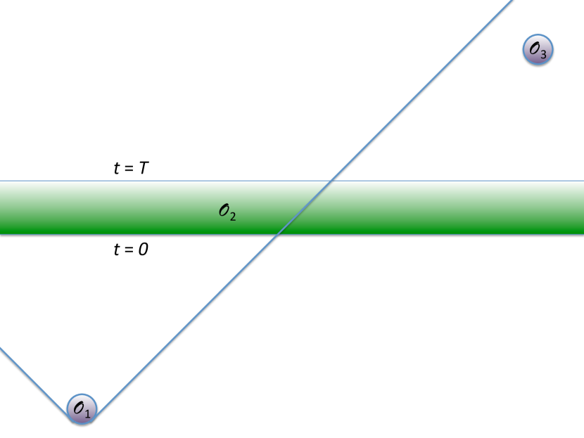
Figure 1: The three intervention regions. In region 1 (a small open ball around spacetime point $X$) we apply a local unitary transformation $e^{i\lambda\hat{\phi}(X)}$. In region 3 (a small open ball around spacetime point $Y$) we measure $\hat{\phi}(Y)$. In region 2 (a slab of spacetime between $t=0$ and $t=T>0$), we consider both ideal measurements of one-particle states and unitary rotations between distinct one-particle states.

Henceforth, we will explicitly consider $(d+1)$-dimensional Minkowski space with a mostly plus metric convention, and a free massless scalar field $\hat{\phi}(x)$, though much of what follows will apply with little or no modification for free massive fields and the general conclusions are relevant in globally hyperbolic spacetimes. Using the formula (1), the following protocol will generally result in superluminal signalling [1]. There are three intervention regions: $\mathcal{O}_{1}$ is a (small open ball around) spacetime point $X^{\mu}$ where $X^{0}\leq 0$, $\mathcal{O}_{2}$ a slab of spacetime between $t=0$ and $t=T>0$ and $\mathcal{O}_{3}$ is a (small open ball around) spacetime point $Y^{\mu}$ spacelike to $X$ and with $Y^{0}\geq T$. See Figure 1. The interventions in these regions are, respectively, a unitary transformation $e^{i\lambda\hat{\phi}(X)}$ where $\lambda$ is a real number, a measurement of $B:=|1\rangle\langle 1|$ where $|1\rangle$ is a one particle state and a measurement of $\hat{\phi}(Y)$.

We pause here to elucidate the meaning of the “measurement of $B$”. $B$ is a projection operator with eigenvalues $1$ and $0$ and what is being measured – putatively – is whether the system is in (Heisenberg) state $|1\rangle$. This observable, which corresponds to a time independent operator, $B$, in the Heisenberg picture, corresponds to a time dependent operator in the Schroedinger picture. For example, if the state corresponds to a one-particle wavepacket – as we will consider in what follows – the observable $B$ corresponds to different positions for the particle at different times as the wavepacket evolves. What is being assumed via formula (1) applied to the protocol described above is that the measurement is achieved by interventions within the slab $\mathcal{O}_{2}$ and the collapse to the eigenstate of $B$ has occurred by the hypersurface $t=T$ so that the measurement at $Y$ with $Y^{0}\geq T$ can take place.

According to (1), the expected value of the outcome of the measurement of $\hat{\phi}(Y)$ depends on $\lambda$ indicating a superluminal signal the strength of which is quantified by [1]

$$S(X,Y):=-{\textrm{Im}}\left(\psi(X)^{*}\psi(Y)\right)$$ (2)

where $\psi(\xi):=\langle 0|\hat{\phi}(\xi)|1\rangle$ is the “one–particle wave-function.” $S(X,Y)$ is the derivative of the expected outcome of the measurement of $\hat{\phi}(Y)$ w.r.t. $\lambda$, at $\lambda=0$, which may be obtained directly by setting $\alpha=0,\beta=1$ in equation (4) of [1]. Fixing spacetime point $X$ so that $\psi(X)$ is real and nonzero, we obtain ${\textrm{Im}}\left(\psi(Y)\right)$ as a measure of the strength of the superluminal signal.

It is straightforward to show that this can be nonzero when the state $|1\rangle$ is a one particle state with a precise $d$-momentum, $\mathbf{k}$. (Spatial $d$-vectors will be written in boldface.) Moreover, in this case the wave-function satisfies $\psi(Y^{\mu}+\xi^{\mu})=\psi(Y^{\mu})$ where $\xi^{\mu}$ is any null vector proportional to the $(d+1)$-momentum, $k^{\mu}=(|\mathbf{k}|,\mathbf{k})$. So the superluminal signal remains no matter how large $T$, no matter how long the measurement-intervention takes. We conclude that an ideal measurement of this single momentum one–particle state is impossible, if superluminal signalling is forbidden (and assuming that the interventions at $X$ and $Y$ can be done). Such a result is not surprising, given the nonlocal character of a fixed momentum state: it is defined on an entire spacelike hypersurface. What might be more surprising is that similar conclusions can be drawn for ideal measurements of localised one–particle wave packet states as we will now show.

Consider the Gaussian one–particle state

$$|1_{d}\rangle:=(\pi\sigma^{2})^{-\frac{d}{4}}\int\,d^{d}{k}\,e^{-\frac{(\mathbf{k}-\mathbf{k}_{0})^{2}}{2\sigma^{2}}}a^{\dagger}_{\mathbf{k}}|0\rangle$$ (3)

where $a^{\dagger}_{\mathbf{k}}$ is the creation operator for a one particle state with $d$-momentum $\mathbf{k}$, $\mathbf{k}_{0}$ is the mean momentum, $\sigma$ is the spread in momentum space and $|\mathbf{k}_{0}|\gg\sigma$.

Consider first $d=1$ and let $k_{0}^{\mu}=k_{0}(1,1)$ where $k_{0}>0$, so the packet is moving in the positive space direction. Then for any null vector $\xi^{\mu}\propto k_{0}^{\mu}$ we have:

$$\begin{array}[]{ll}\psi(Y^{\mu}+\xi^{\mu})&=\langle 0|\hat{\phi}(Y^{\mu}+\xi^{\mu})|1_{1}\rangle\\ &=(\pi\sigma^{2})^{-\frac{1}{4}}\int_{-\infty}^{\infty}\frac{dk}{4\pi|k|}e^{-\frac{(k-k_{0})^{2}}{2\sigma^{2}}}e^{ik_{\mu}(Y^{\mu}+\xi^{\mu})}\,.\end{array}$$ (4)

To avoid the pole at the origin, let us modify the wavepacket slightly, allowing it to have support in momentum space only for $k>\epsilon>0$ where $\epsilon$ is small. Then for all momenta contributing to the integral we have $k_{\mu}\xi^{\mu}=0$ and, hence,

$$\psi(Y^{\mu}+\xi^{\mu})=\psi(Y^{\mu})\,.$$ (5)

In $1+1$ dimensions, when the packet has support only on momenta in the positive spatial direction, it holds its form, does not spread and the superluminal signal persists undiminished for arbitrary intervention time, $T$: $Y$ can be chosen in the support of the packet and such that $Y^{0}=T$ and ${\textrm{Im}}(\psi(Y))\neq 0$. Note that this result holds for any packet with support only on positive momenta – the approximately Gaussian form is not necessary.

The quantum theory of a massless scalar field in $1+1$ dimensional Minkowski spacetime is unphysical, not least because it suffers from an infrared divergence, so we turn our attention to $3+1$ dimensions. The same conclusion obtained in $1+1$ dimensions about persistence of the signal holds in $3+1$ dimensions if the wavepacket is completely spatially delocalised in the directions transverse to the direction of motion of the packet which is in the positive $z$-direction, say. In other words, the packet has support in momentum space on fixed values of the momentum in the $x$ and $y$ directions and a spread of positive values of the momentum in the $z$ direction. In the more physical case, when the packet is localised in all three spatial dimensions and described by the state $|1_{3}\rangle$ in (3), the amplitude of the envelope of the packet will decay due to diffraction into the transverse directions. Thus, in $3+1$ dimensions the particular measure of the superluminal signal, ${\textrm{Im}}(\psi(Y))$, decays as $Y^{0}=T$ – the intervention time – increases. To make this concrete, let us consider the Gaussian packet $|1_{3}\rangle$ peaked at $\mathbf{k}_{0}=(0,0,k_{0})$ and calculate $\psi(Y)$ for arbitrary points in the $z-t$ plane, $Y=(t,0,0,z)$. Then $\psi(Y)$ can be evaluated in closed form [3, § 3.953]:

$$\begin{array}[]{cl}\psi(Y)=\langle 0|\hat{\phi}(t,0,0,z)|1_{3}\rangle&=(\pi\sigma^{2})^{-\frac{3}{4}}\int\frac{d^{3}k}{(2\pi)^{\frac{3}{2}}\sqrt{2|\mathbf{k}|}}e^{-\frac{(\mathbf{k}-\mathbf{k}_{0})^{2}}{2\sigma^{2}}}e^{ik_{\mu}Y^{\mu}}\\ &=\frac{e^{-k_{0}^{2}/2\sigma^{2}}}{4\pi^{\frac{3}{4}}}\frac{e^{v_{-}^{2}/4}D_{-\frac{3}{2}}\left(v_{-}\right)-e^{v_{+}^{2}/4}D_{-\frac{3}{2}}\left(v_{+}\right)}{k_{0}\sigma^{-2}+iz},\end{array}$$ (6)

where $v_{\pm}=i\sigma\left[t\pm(z-ik_{0}/\sigma^{2})\right]$ and $D_{\nu}(z)$ is the parabolic cylinder function.

In Figure 2, the imaginary part of $\psi(t,0,0,z)$ for the Gaussian $1-$particle state with $\mathbf{k}_{0}=(0,0,10)$ and $\sigma=1$ is plotted as a function of $z$ for $t=0,10,20$. It can be seen that the amplitude of the packet envelope remains non-negligible for values of $t=Y^{0}$ which are a few times the spatial width of the packet. If we choose $X$ to be at the origin, $X^{\mu}=(0,0,0,0)$, then at each of the representative times, points in the right hand half of the support of the packet are spacelike to $X$. Therefore $Y$ can be spacelike to $X$, in the support of the packet and such that $Y^{0}=$ few$\times$(spatial extent of packet) and the measure of the superluminal signal $\textrm{Im}(\psi(Y))$ is non-negligible. Indeed, if we let $z=t+\delta$ with $0<\delta<1/\sigma$, such that $Y$ is spacelike to $X$ but still inside the support of the wavepacket, then the asymptotic expansion of (6) for large $t\gg k_{0}/\sigma^{2}$ gives [4]:

$${\textrm{Im}}(\psi(Y))\sim\gamma\sqrt{k_{0}/\sigma}\cos(k_{0}\delta)t^{-1}$$ (7)

where $\gamma$ is a constant of order $\mathcal{O}(10^{-1})$. It follows that the envelope of the superluminal signal $\textrm{Im}(\psi(Y))$ falls off like $t^{-1}$.

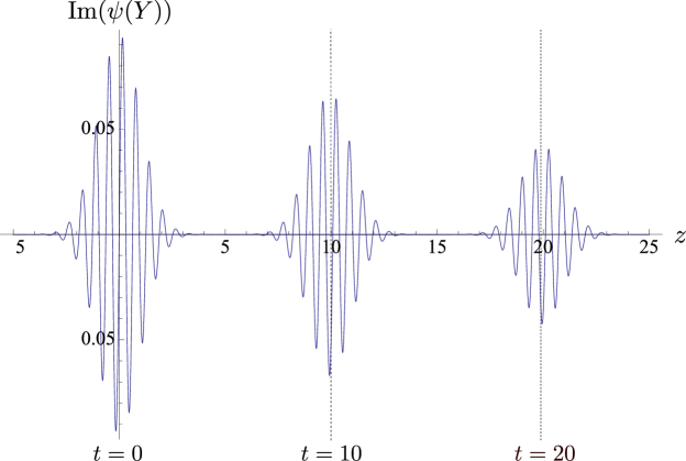
Figure 2: The imaginary part of $\psi(t,0,0,z)$ for the Gaussian $1-$particle state with $\mathbf{k}_{0}=(0,0,10)$ and $\sigma=1$, plotted as a function of $z$ for different values of $t=0,10,20$.

We conclude that one or more of the three interventions – the unitary kick at $X$, the ideal measurement of the wavepacket between $t=0$ and $t=T=$few$\times$(spatial size of packet), or the measurement of $\hat{\phi}(Y)$ – is impossible. The measurement of the wavepacket is the most questionable but to begin to address these questions properly we need to model the interventions physically.

The same no-go results apply to unitary transformations: an intervention by an external agent that produces a nonlocal unitary transformation on the state of the field, for example, a unitary transformation that rotates the state from one 1–particle state to an orthogonal 1–particle state, can enable superluminal signalling. Consider the $2-$dimensional Hilbert space $\mathcal{H}$ spanned by two 1–particle states $|1\rangle$ and $|1^{\prime}\rangle$. This space is a subspace of the Fock space $\mathcal{F}=\mathcal{H}\oplus\mathcal{H}^{\perp}$ of the scalar field and $\mathcal{H}^{\perp}$ denotes its orthogonal complement. The field starts in a state $|\psi\rangle=A|1\rangle+B|1^{\prime}\rangle$. Consider the same 3 intervention regions, $\mathcal{O}_{1}$, $\mathcal{O}_{2}$ and $\mathcal{O}_{3}$, as before. A local unitary operation $e^{i\lambda\hat{\phi}(X)}$ is done at $X$ followed by a unitary operation $U$ done in $\mathcal{O}_{2}$ where

$$\!U=e^{i\theta}(C|1\rangle\!\langle 1|+D|1\rangle\!\langle 1^{\prime}|-D^{*}|1^{\prime}\rangle\!\langle 1|+C^{*}|1^{\prime}\rangle\!\langle 1^{\prime}|)+\mathbf{1}^{\perp}\,,\vphantom{\int}$$ (8)

$|C|^{2}+|D|^{2}=1$ and $\mathbf{1}^{\perp}$ is the identity operator on $\mathcal{H}^{\perp}$. Finally, $\hat{\phi}(Y)$ is measured at $Y$. The expected value of the measurement of $\hat{\phi}(Y)$ is

$$\langle\hat{\phi}(Y)\rangle=\langle\psi|e^{-i\lambda\hat{\phi}(X)}U^{\dagger}\hat{\phi}(Y)Ue^{i\lambda\hat{\phi}(X)}|\psi\rangle\,.$$ (9)

Differentiating w.r.t. $\lambda$ and setting $\lambda=0$ we find that the superluminal signal is nonzero if the following expression is nonzero:

$$2{\textrm{Im}}\langle\psi|\hat{\phi}(X)U^{\dagger}\hat{\phi}(Y)U|\psi\rangle\,.$$ (10)

For $A=1$, $B=0$, $C=0$ and $D=-1$ we find

$$\langle\psi|\hat{\phi}(X)U^{\dagger}\hat{\phi}(Y)U|\psi\rangle=\psi(X)^{*}\psi^{\prime}(Y)+\psi^{\prime}(X)\psi(Y)^{*}$$ (11)

where $\psi(\xi)=\langle 0\,|\hat{\phi}(\xi)|\,1\rangle$ and $\psi^{\prime}(\xi)=\langle 0\,|\hat{\phi}(\xi)|\,1^{\prime}\rangle$ are the one particle wave functions.

If the one particle states are single momentum states, this is easily worked out. Let us work in a box of side length $L$, so that

$$\hat{\phi}(X)=L^{-\frac{d}{2}}\sum_{\mathbf{k}}\frac{1}{\sqrt{2\omega_{\mathbf{k}}}}\left[a_{\mathbf{k}}^{\vphantom{\dagger}}u^{\vphantom{\dagger}}_{\mathbf{k}}(X)+a_{\mathbf{k}}^{\dagger}u^{*}_{\mathbf{k}}(X)\right]$$ (12)

where $u_{\mathbf{k}}(X)=e^{ik_{\mu}X^{\mu}}$. Let $|1\rangle=a_{\mathbf{k}}^{\dagger}|0\rangle$ and $|1^{\prime}\rangle=a_{\mathbf{k}^{\prime}}^{\dagger}|0\rangle$. Then the signal (10) evaluates to

$$\!\!\!\!\!\!\frac{L^{-d}}{\sqrt{\omega_{\mathbf{k}}\omega_{\mathbf{k}^{\prime}}}}\left[\sin(k^{\prime}_{\mu}Y^{\mu}-k_{\mu}X^{\mu})-\sin(k_{\mu}Y^{\mu}-k^{\prime}_{\mu}X^{\mu})\right].$$ (13)

This can be nonzero for spacelike separated $X$ and $Y$. For example, for $\mathbf{k}=-\mathbf{k}^{\prime}$ we obtain

$$-\frac{2L^{-d}}{\omega_{\mathbf{k}}}\sin\left[\omega_{\mathbf{k}}(Y^{0}-X^{0})\right]\cos\left[\mathbf{k}\cdot(\mathbf{Y}+\mathbf{X})\right],$$ (14)

which is nonzero for choices of spacelike separated $Y$ and $X$ for which $Y^{0}-X^{0}$ is arbitrarily large. If $|1\rangle$ and $|1^{\prime}\rangle$ are wave packet states, the spreading of the packets becomes relevant. However, similarly to the previous calculation, $X$ can be chosen in the support of $\psi$ at $t=0$ and $Y$ in the support of $\psi^{\prime}$ at $t=T$ and there will be superluminal signalling for $T=$few$\times$(width of packet). Unitary transformations that would apparently not violate relativistic causality are those which are products of unitaries that are perfectly localised at spacetime points on a spacelike hypersurface, e.g. $e^{i\int d^{d}xf({\mathbf{x}})\hat{\phi}(t,\mathbf{x})}$.

3 Different rules

The preceding observations show that modelling external interventions on quantum fields as ideal measurements and unitary transformations in a straightforward generalisation of the text-book, operational rules for nonrelativistic quantum theory fails. One response could be to put restrictions on the use of the formula (1) for the probabilities of outcomes of a collection of measurements.

Restricting the regions. One could require that the relation $\preceq$ between the intervention regions, $\mathcal{O}_{i}$, is already a partial order before the transitive closure is taken [1]. In the protocol considered above that would require $X$ to be in the causal past of $Y$ and any signalling would then be causal by fiat. This leaves the question, “What is the probability of a certain sequence of outcomes of measurement-interventions in regions which are not partially ordered?” without any answer, though there seems to be no physical reason why the relative positions of the regions in spacetime should affect agents’ ability to do measurements in them. Other, even more restrictive conditions on the regions $\mathcal{O}_{i}$ might be considered. For example, one might require that for every pair $(\mathcal{O}_{j},\mathcal{O}_{k})$ such that $j<k$, either the two regions are entirely spacelike to each other or every point of $\mathcal{O}_{j}$ is in the causal past of every point of $\mathcal{O}_{k}$ [1]. Once again, such rules would be silent on how to make predictions when the interventions on quantum fields take place in regions that do not satisfy these conditions.

Restricting the observables. Alternatively one could leave the regions unrestricted and use the criterion that no superluminal signalling is allowed to place conditions on the observables to which (1) is to apply, the approach taken in [5, 6, 7, 8]. Beckman et al. [9] comprehensively analyse the restriction that causality places on “quantum operations” – including ideal measurements and unitary transformations as special cases – on bipartite systems with tensor product Hilbert spaces.

In quantum field theory, a particularly important example of a physical quantity that cannot be measured by an ideal measurement without causing superluminal signalling is a non-abelian Wilson loop [10]. This seems to leave non-abelian gauge theory with no physical, gauge invariant “measureables” at all! In scalar field theory, the situation seems not to be so dire. There is a class of observables which, should they be measurable by ideal measurements, would not causal superluminal signals: integrals over spacelike hypersurfaces of local field operators and their conjugate momentum operators, such as those considered in [11]. At least, this is the conclusion one would draw by analogy with the result for a bipartite, tensor product system that an ideal measurement of a sum of local observables does not violate causality. For completeness, let us demonstrate this result. Let $H=H_{1}\otimes H_{2}$ be a tensor product Hilbert space and let $A$ and $B$ be self-adjoint operators on $H_{1}$ and $H_{2}$ respectively. Suppose the system is initially in state $\rho_{0}$ and we consider the following protocol: a local unitary operation, $U_{1}$ on $H_{1}$, followed by a measurement of $X=A+B$. We use the observation [1] that the effect of a measurement of $X$ on the state is achieved by application of the unitary operator $e^{i\lambda X}$ with a random value of $\lambda$. $A$ and $B$ commute and so $e^{i\lambda X}=e^{i\lambda A}e^{i\lambda B}$ which is a product of local unitaries which commute. Now consider the operation $U_{1}$ followed by application of $e^{i\lambda A}e^{i\lambda B}$ followed by a partial trace over $H_{1}$, all on the state $\rho_{0}$. The reduced state for $H_{2}$ does not depend on $U_{1}$.

This result suggests that in QFT no violation of relativistic causality would result from the ideal measurement of the (Heisenberg) observable $a_{\mathbf{k}}(t)+a_{\mathbf{k}}^{\dagger}(t)=a_{\mathbf{k}}e^{-i\omega_{\mathbf{k}}t}+a_{\mathbf{k}}^{\dagger}e^{i\omega_{\mathbf{k}}t}$, where $\omega_{\mathbf{k}}$ is the frequency for momentum $\mathbf{k}$, which may be written as

$$a_{\mathbf{k}}(t)+a_{\mathbf{k}}^{\dagger}(t)=\int d^{d}x\,\hat{\phi}(t,{\mathbf{x}})F(\mathbf{x})+\int d^{d}x\,\hat{\pi}(t,{\mathbf{x}})G(\mathbf{x})$$ (15)

where $\hat{\pi}$ is the canonical momentum of $\hat{\phi}$, and

$$\begin{array}[]{ll}F(\mathbf{x})=(2\omega_{\mathbf{k}})^{\frac{1}{2}}(2\pi)^{-\frac{d}{2}}\cos\mathbf{k}\cdot\mathbf{x}\\ G(\mathbf{x})=\left(\frac{2}{\omega_{\mathbf{k}}}\right)^{\frac{1}{2}}(2\pi)^{-\frac{d}{2}}\sin\mathbf{k}\cdot\mathbf{x}\,.\end{array}$$ (16)

To make the single momentum states normalised by working in a box of side length $L$, we could replace the $(2\pi)$ by $L$ in (16) and (16). Although this observable is defined on the whole constant time hypersurface at $t$ it is a sum of truly local terms on the hypersurface. It is “essentially local” but not “localised” and therefore unlikely to be useful for QIP in Minkowski space. Localised smearings, such as those considered in [11], have a better chance of being useful.

Another example of a more localised observable is $b(t)+b^{\dagger}(t)$ where $b^{\dagger}(0)$ is defined by $b^{\dagger}(0)|0\rangle=|1\rangle$, a one particle wave packet state. If

$$b^{\dagger}(0)=\int d^{d}k\,\tilde{\psi}(\mathbf{k})\,a^{\dagger}_{\mathbf{k}}$$ (17)

then the one particle wave function is

$$\psi(t,\mathbf{x})=\int d^{d}k\,(2\omega_{\mathbf{k}})^{-\frac{1}{2}}(2\pi)^{-\frac{d}{2}}e^{i\mathbf{k}\cdot\mathbf{x}}e^{-i\omega_{\mathbf{k}}t}\tilde{\psi}(\mathbf{k})$$ (18)

and

$$b(t)+b^{\dagger}(t)=\int d^{d}x\,\left(\hat{\phi}(t,{\mathbf{x}})J(\mathbf{x})+\hat{\pi}(t,{\mathbf{x}})K(\mathbf{x})\right)$$ (19)

where

$$\begin{array}[]{lcrlll}J(\mathbf{x})&=&\int\frac{d^{d}k}{(2\pi)^{\frac{d}{2}}}\left(\frac{\omega_{\mathbf{k}}}{2}\right)^{\frac{1}{2}}&\left[e^{i\mathbf{k}\cdot\mathbf{x}}\tilde{\psi}(\mathbf{k})+{\textrm{c.c.}}\right]\\ K(\mathbf{x})&=&-i\int\frac{d^{d}k}{(2\pi)^{\frac{d}{2}}(2\omega_{\mathbf{k}})^{\frac{1}{2}}}&\left[e^{i\mathbf{k}\cdot\mathbf{x}}\tilde{\psi}(\mathbf{k})-{\textrm{c.c.}}\right].\end{array}$$ (20)

$K(\mathbf{x})$ is (twice) the imaginary part of $\psi(0,\mathbf{x})$ but $J(\mathbf{x})$ is not its real part.

We see that for $b(t)+b^{\dagger}(t)$ to be localised, $\tilde{\psi}(\mathbf{k})$ must be such that $K$ and $J$ have bounded support in space. $K$ will do so if the one-particle wavefunction $\psi$ at $t=0$ does but requiring $J$ to have bounded support imposes an additional constraint and it is not clear that both constraints can be exactly satisfied. If it is sufficient for $K$ and $J$ to be exponentially small outside a bounded region of space then the Gaussian wave packet state (3) will do, but, strictly, to measure $b(t)+b^{\dagger}(t)$ in this case requires an intervention region that includes the whole spacelike hypersurface at $t$. If we accept that in this case intervening in a bounded region can in principle result in an ideal measurement of $b(t)+b^{\dagger}(t)$ to a very good approximation, it is still an open question whether it can be measured by an ideal measurement in practice.

The observables on which the algebraic approach to relativistic quantum field theory is based are field operators smeared with test functions with bounded spacetime support and Sorkin raised the question whether or not ideal measurements of such observables would enable superluminal signalling [1]. We note that for a free scalar field, since the field operators $\hat{\phi}(X)$ and $\hat{\pi}(X)$ at any spacetime point $X$ are linear combination of the field operators and the conjugate momentum operators on the intersection of any spacelike hypersurface, $\Sigma$ and the causal past of $X$, such a spacetime smearing of a free field is equal to a spatial smearing of local operators over $\Sigma$. This suggests that an ideal measurement of a spacetime smearing of a free field would not enable superluminal signalling. Of course, no field can be truly free, if only because measurements must be modelled by interactions, and for an interacting field, the question remains open.

4 Detector models

A more physical approach to addressing these questions – and, for example, explaining which of the interventions considered in the first section is impossible – is to construct explicit models of the interventions and measurements as interactions between the field and other quantum systems. A quantum detector for example could act as the ‘qubit’ that is manipulated by the classical agent and the quantum field coupled to it would then be part of the quantum system that performs the processing task but would not be directly intervened upon by the external agent. A detector would have a world-line or world-volume in spacetime and one would have to assume that ideal measurements and unitary transformations can be performed on it by the external agent in some region.

One prototype of such a detector is the Unruh-DeWitt (UD) detector [12, 13]. UD detectors and their ilk couple to the field operator itself and field operators at spacelike separated positions commute. It is an interesting question whether there is any observable in the quantum field theory that can be said to be measured by an UD detector, but here we simply note that signalling between two UD detectors will not occur if their world-volumes are completely spacelike separated while they are switched on, and (1) is used for the probability of ideal measurements on the detectors themselves [14]. Whether UD detectors are good models of realistic detectors that can be used in QIP is an open question. In order to provide a useful qubit a UD detector needs to be switched on and off at finite times and also itself prepared and measured or manipulated at finite times. This requires the modelling of the switching process to be addressed with care [15] but at least relativistic causality can be safe with UD detectors because they couple locally to the field.

Are there other model detectors that might be applicable to QIP in Minkowski spacetime? We briefly consider two that appear in the literature. A detector that couples to one single frequency mode of a scalar field in 1+1 dimensions is investigated in [16, 17]. We can imagine that the system is in a large box of size $L$ with periodic boundaries, say, so that the single mode state is normalisable. The Hamiltonian for the model is

$$\hat{H}(t)={w}({\hat{d}}^{\dagger}{\hat{d}}+\frac{1}{2})+\Omega({\hat{f}}^{\dagger}{\hat{f}}+\frac{1}{2})+\lambda(t)(\hat{d}+\hat{d}^{\dagger})\left(\hat{f}e^{i\Omega x}+\hat{f}^{\dagger}e^{-i\Omega x}\right),$$ (21)

where $x$ is the position of the detector which has an internal harmonic oscillator degree of freedom with frequency $w$ and raising operator $\hat{d}^{\dagger}$, and $\Omega$ is the frequency of the field mode with one-particle creation operator $\hat{f}^{\dagger}$. This causes superluminal signalling if interpreted as a model for a localised detector interacting with a field in Minkowski spacetime, or in a box such that the light crossing time of the box is longer than the timescale on which the model is valid.

Consider, following [17], the particular case of two static detectors at positions $x_{i}$, with frequencies $w_{i}$ and couplings $\lambda_{i}(t)$, $i=1,2$. In order that the model be close to Minkowski spacetime, we assume that the box size $L$ is large compared to $|x_{1}-x_{2}|$. In the interaction picture, the interaction Hamiltonians are

$$H_{i,{\textrm{int}}}(t)=\lambda_{i}(t)(\hat{d}_{i}e^{-i\omega_{i}t}+\hat{d}_{i}^{\dagger}e^{i\omega_{i}t})\left(\hat{f}e^{i\Omega(x_{i}-t)}+\hat{f}^{\dagger}e^{-i\Omega(x_{i}-t)}\right)$$ (22)

for $i=1,2$. The time dependence in $\lambda_{i}(t)$ parametrizes the switching on and off of the detectors. The interaction Hamiltonians of the two detectors at spacelike separated positions do not commute. Indeed, defining $X_{i}^{\mu}:=(t_{i},x_{i})$ and $\Omega^{\mu}:=(\Omega,\Omega)$, we have the commutator

$$\begin{array}[]{lcl}[H_{1,{\textrm{int}}}(t_{1}),H_{2,{\textrm{int}}}(t_{2})]&=&-2i\lambda_{1}(t_{1})\lambda_{2}(t_{2})(\hat{d}_{1}e^{-i\omega_{1}t_{1}}+\hat{d}_{1}^{\dagger}e^{i\omega_{1}t_{1}})\times\\ &&~{}~{}(\hat{d}_{2}e^{-i\omega_{2}t_{2}}+\hat{d}_{2}^{\dagger}e^{i\omega_{2}t_{2}})\sin{\Omega_{\mu}(X_{1}-X_{2})^{\mu}}\,.\end{array}$$ (23)

This is nonzero for almost every pair of spacetime points along the trajectories of two detectors which are spacelike separated. This means that the unitary evolution operator in the interaction picture does not factorise into a product of an evolution operator for detector 1 and one for detector 2 and this leads to superluminal signalling between the detectors as we show explicitly below.

Let both detectors and the scalar field be initially in their free ground states at $t=0$ and assume that the detectors are switched off before $t=0$: $\lambda_{i}(t)=0$ for $t<0$. Working in the interaction picture, at time $T>0$ we measure for detector 1 the expectation value, denoted $E_{1}(T)$, of the operator

$$\mathcal{O}(T)=\omega_{1}(\hat{d}_{1}(T)^{\dagger}\hat{d}_{1}(T)+\frac{1}{2})=\omega_{1}(\hat{d}_{1}^{\dagger}\hat{d}_{1}+\frac{1}{2}).$$ (24)

$E_{1}(T)$ ought to be independent of $\lambda_{2}$ so long as detector 1 remains outside the causal future of the point $(0,x_{2})$, i.e. when $T<|x_{2}-x_{1}|$. Otherwise, an observer at $(T,x_{1})$ could use their detector to infer whether spacelike separated detector 2 has been switched on or not (i.e. whether $\lambda_{2}\neq 0$ or not). We do not carefully model the switching process and simply take $\lambda_{i}(t)$ to be a step function, constant and nonzero only in the interval $0<t\leq T$ and then $E_{1}(T)$ can be evaluated explicitly using the Heisenberg Picture analysis presented in [17]. It can be shown that $E_{1}(T)$ does in general depend on $\lambda_{2}$, and by way of example let us evaluate it for a specific set of values: $w_{1}=w_{2}=\Omega=1$, $\lambda_{1}=\frac{1}{2}$, $x_{1}=0$ and $x_{2}=2\pi$. With a constant coupling $\lambda_{2}(t)=\lambda_{2}$ for $0<t\leq T=\sqrt{2}\pi<|x_{2}-x_{1}|$ one obtains

$$E_{1}(\sqrt{2}\pi)=\frac{1}{4}\left(2+\pi^{2}\right)+\frac{1}{3}\pi^{4}\lambda_{2}^{2}+\mathcal{O}(\lambda_{2}^{4}).$$ (25)

We see a second–order dependence on the coupling constant $\lambda_{2}$ of detector 2 – a superluminal signal.

The signalling observed in the case of finite mode coupling becomes more comprehensible if the detector is interpreted as a variant of an UD detector in which the detector couples both to the field and to its conjugate momentum. Indeed, modifying the calculation that leads to (15), we find for the factor in the interaction hamiltonian $H_{1,{\textrm{int}}}(t)$ for the first detector

$$\hat{f}e^{i\Omega(x_{1}-t)}+\hat{f}^{\dagger}e^{-i\Omega(x_{1}-t)}=\int dx\hat{\phi}(t,x)F_{1}(x)+\int dx\hat{\pi}(t,x)G_{1}(x)$$ (26)

where

$$\begin{array}[]{lcl}F_{1}(x)&=&(2\Omega)^{\frac{1}{2}}L^{-\frac{1}{2}}\cos[{\Omega(x-x_{1})}]\\ G_{1}(x)&=&\left(\frac{2}{\Omega}\right)^{\frac{1}{2}}L^{-\frac{1}{2}}\sin[{\Omega(x-x_{1})}]\,.\end{array}$$ (27)

We can see that the effective spatial extension of the detector is not bounded: the detector is not localised and two detectors which are nominally spacelike separated actually overlap over all space.

In [18] a more ambitious model of a detector defined using additional quantum fields coupled to the field being measured is considered. Since the interaction between the fields is local no superluminal signalling can be enabled as a result of the interaction in and of itself. If taken literally, the effective model of the detector given in equation (14) in [18] looks like it does enable superluminal signalling since the interaction Hamiltonians of two detectors centred at spacelike separated positions do not commute. Just as in the calculation above, this will result in the response of one detector depending on whether or not there exists a second one spacelike to it. Again, this happens because detectors constructed as described in [18] cannot be genuinely spacelike separated: they may be centred around localised positions but will always have some spatial overlap. The authors themselves state that the detector is nonlocal. However, the question of whether the state of such a detector itself is measurable by an ideal measurement immediately arises: does an ideal measurement on the non-local detector enable superluminal signalling? This is not addressed in [18] but it should not be hard to determine.

5 Cavities

Those familiar with cavity QED might be surprised at these results. After all, in a cavity, ideal measurements of observables such as particle number can be done [19] and there’s a well-known, successful model of an atom-qubit interacting with QED in a cavity which is of the form investigated above in which a detector couples to a single mode of the field: the Jaynes-Cummings model (see e.g [20] for a review). The reason there is no conflict with the results presented here is that the Jaynes-Cummings model is a phenomenological model which applies only on time scales many orders of magnitude larger than the light crossing time of the cavity. It does not describe the physics on time scales of order the light crossing time or shorter. If there are two atoms in a cavity, they cannot be placed further apart than the size of the cavity and so their worldlines cannot remain spacelike to each other on the time scales on which the Jaynes-Cummings model applies and so no possibility of superluminal signalling arises in the model.

The Jaynes-Cummings Hamiltonian and its relatives cannot model an atom-qubit coupled to a quantum field in Minkowski spacetime, or in any spacetime where two atom-qubits can be placed at distances larger than the timescale on which the detector model is valid. A model detector such as that considered in [16, 17] would not do violence to relativistic causality if it were interpreted phenomenologically and confined to a spacetime of much smaller spatial extent than the timescale on which the model is valid since this would effectively impose a non-relativistic causal order on the intervention-events in the cavity. In the light of the phenomenological successes of such models, one might be tempted to declare more widely that QFT is only physical in a box and that intervention regions $\mathcal{O}_{i}$ must always have extent in time at least the light-crossing time of the box, imposing a non-relativistic causal order on interventions on the field. Such a rule would be highly restrictive and could not accommodate the questions that arise when the operations of the external agents on a quantum field take place in arbitrary, quasi-local spacetime regions, exactly the sort of situation that a genuinely relativistic approach to QIP aims to describe.

6 Concluding Remarks

The questions remain. What are accurate models of physical interventions on relativistic quantum fields in quasi-local regions of Minkowski spacetime and what applications might they have in QIP? Localised Unruh-DeWitt type detectors form one class of models: Are they realistic? Are there others? The questions are interesting from the point of view of QIP but also because the attempt to answer them pushes us to address more foundational issues. The struggle to describe measurement of relativistic quantum fields in a physical way reveals the limitations of the canonical and operational approach to quantum theory. Even when a detector is modelled as a quantum system, to be a useful qubit one still has to rely on the assumption that an external agent can measure it by an ideal measurement and/or do unitary transformations on it. But a more fundamental description of the detector – and indeed the agent – would be in terms of quantum field theory and so one is not solving the problem but just pushing it one step away: how would one model the effect of an ideal measurement on the detector if the detector were described within a quantum field theory (cf. [18])?

A more physical approach is needed: we require a framework for closed relativistic quantum systems including detectors, in which experimental, measurement-like situations can be analysed fully quantum mechanically in an essentially relativistic way.

One proposal for such a framework takes the relativistic branch of the ‘fork in the road’ set out by Dirac early in the history of quantum mechanics. In the 1933 paper, “The Lagrangian in quantum mechanics,” Dirac wrote that the Lagrangian approach to classical mechanics is probably more fundamental than the Hamiltonian approach because the former is relativistically invariant whereas the latter is “essentially nonrelativistic” [21]. In quantum theory the Hamiltonian approach leads to canonical quantisation, Hilbert space, operators, observables, transformation theory and the textbook rules for predicting the outcomes of measurements of observables and for the collapse of the state after an ideal measurement. These aspects of the canonical theory are indeed more or less divorced from the spacetime nature of the physical world revealed by relativity.

The relativistic alternative is to base quantum mechanics on the Lagrangian approach to classical mechanics and Dirac showed that this leads to the path integral [21]. The path integral roots quantum theory firmly in spacetime – rather than Hilbert space – as the arena for physics. In a path integral or sum-over-histories approach, the physical world is described directly in terms of events in spacetime and Feynman’s famous paper on the path integral is aptly titled “The spacetime approach to non-relativistic quantum mechanics”[22]. The path integral approach to the foundations of quantum theory has been championed in more recent times by Hartle [23, 24] and by Sorkin [25]. In [26] measurement situations in closed quantum systems are analysed from a sum-over-histories perspective, with an emphasis on a condition of decoherence. In [27] a solution of the “measurement problem” of quantum mechanics is set out which is valid, at least, when there are certain sorts of permanent records of measurement outcomes. As a framework for closed quantum systems which deals directly with spacetime events, the path integral approach is eminently suitable for the investigation of measurements on relativistic quantum fields in Minkowski spacetime.

References

References

- [1] Rafael D. Sorkin. Impossible measurements on quantum fields. In Directions in General Relativity: Volume 2: Proceedings of the 1993 International Symposium, Maryland: Papers in Honor of Dieter Brill, volume 1, page 293. Cambridge University Press, 1993.
- [2] K.E. Hellwig and K. Kraus. Formal description of measurements in local quantum field theory. Phys.Rev., D1:566–571, 1970.
- [3] Alan Jeffrey and Daniel Zwillinger. Table of integrals, series, and products. Academic Press, 2007.
- [4] Daniel W Lozier. Nist digital library of mathematical functions. Annals of Mathematics and Artificial Intelligence, 38(1-3):105–119, 2003.
- [5] Yakir Aharonov and David Z. Albert. States and observables in relativistic quantum field theories. Phys. Rev. D, 21:3316–3324, Jun 1980.
- [6] Yakir Aharonov and David Z. Albert. Can we make sense out of the measurement process in relativistic quantum mechanics? Phys. Rev. D, 24:359–370, Jul 1981.
- [7] Yakir Aharonov, David Z. Albert, and Lev Vaidman. Measurement process in relativistic quantum theory. Phys. Rev. D, 34:1805–1813, Sep 1986.
- [8] Yakir Aharonov and Daniel Rohrlich. Quantum Paradoxes, chapter 14, pages 193–209. Wiley-VCH Verlag GmbH, 2008.
- [9] David Beckman, Daniel Gottesman, M.A. Nielsen, and John Preskill. Causal and localizable quantum operations. Phys.Rev., A64:052309, 2001.
- [10] David Beckman, Daniel Gottesman, Alexei Kitaev, and John Preskill. Measurability of Wilson loop operators. Phys.Rev., D65:065022, 2002.
- [11] Magdalena Zych, Fabio Costa, Johannes Kofler, and Caslav Brukner. Entanglement between smeared field operators in the Klein-Gordon vacuum. Phys.Rev., D81:125019, 2010.
- [12] W.G. Unruh. Notes on black hole evaporation. Phys.Rev., D14:870, 1976.
- [13] Bryce S DeWitt. Quantum gravity: the new synthesis. In General relativity: an Einstein centenary survey, volume 1, pages 680–745. Cambridge University Press, 1979.
- [14] M. Cliche and A. Kempf. Relativistic quantum channel of communication through field quanta. Phys. Rev. A, 81:012330, Jan 2010.
- [15] Jorma Louko and Alejandro Satz. Transition rate of the Unruh-DeWitt detector in curved spacetime. Class.Quant.Grav., 25:055012, 2008.
- [16] Eduardo Martin-Martinez, Ivette Fuentes, and Robert B. Mann. Using Berry’s phase to detect the Unruh effect at lower accelerations. Phys.Rev.Lett., 107:131301, 2011.
- [17] Andrzej Dragan and Ivette Fuentes. Probing the spacetime structure of vacuum entanglement. arXiv preprint arXiv:1105.1192, 2011.
- [18] Fabio Costa and Federico Piazza. Modelling a Particle Detector in Field Theory. New J.Phys., 11:113006, 2009.
- [19] BR Johnson, MD Reed, AA Houck, DI Schuster, Lev S Bishop, E Ginossar, JM Gambetta, L DiCarlo, L Frunzio, SM Girvin, et al. Quantum non-demolition detection of single microwave photons in a circuit. Nature Physics, 6(9):663–667, 2010.
- [20] R Miller, TE Northup, KM Birnbaum, ADBA Boca, AD Boozer, and HJ Kimble. Trapped atoms in cavity qed: coupling quantized light and matter. Journal of Physics B: Atomic, Molecular and Optical Physics, 38(9):S551, 2005.
- [21] Paul AM Dirac. The lagrangian in quantum mechanics. Physikalische Zeitschrift der Sowjetunion, 3(1):64–72, 1933.
- [22] Richard Phillips Feynman. Space-time approach to non-relativistic quantum mechanics. Reviews of Modern Physics, 20(2):367, 1948.
- [23] James B. Hartle. The Space-time approach to quantum mechanics. Vistas Astron., 37:569, 1993.
- [24] JB Hartle. Spacetime quantum mechanics and the quantum mechanics of spacetime. In Gravitation and Quantizations, Session LVII of Les Houches, volume 1, page 285, 1995.
- [25] D. Sorkin, Rafael. Quantum mechanics as quantum measure theory. Mod.Phys.Lett., A9:3119–3128, 1994.
- [26] James B Hartle. The reduction of the state vector and limitations on measurement in the quantum mechanics of closed systems. In Directions in General Relativity: Volume 2: Proceedings of the 1993 International Symposium, Maryland: Papers in Honor of Dieter Brill, volume 1, page 129. Cambridge University Press, 1993.
- [27] Rafael D Sorkin. Logic is to the quantum as geometry is to gravity⋆. Foundations of Space and Time: Reflections on Quantum Gravity, page 363, 2012.