Fast Variational Inference in the Conjugate Exponential Family

Abstract

We present a general method for deriving collapsed variational inference algorithms for probabilistic models in the conjugate exponential family. Our method unifies many existing approaches to collapsed variational inference. Our collapsed variational inference leads to a new lower bound on the marginal likelihood. We exploit the information geometry of the bound to derive much faster optimization methods based on conjugate gradients for these models. Our approach is very general and is easily applied to any model where the mean field update equations have been derived. Empirically we show significant speed-ups for probabilistic inference using our bound.

1 Introduction

Variational bounds provide a convenient approach to approximate inference in a range of intractable models. Classical variational optimisation is achieved through coordinate ascent which can be slow to converge. A popular solution (King and Lawrence, 2006; Teh et al., 2007; Kurihara et al., 2007; Sung et al., 2008; Lázaro-Gredilla and Titsias, 2011; Lázaro-Gredilla et al., 2011) is to marginalize analytically a portion of the variational approximating distribution, removing this from the optimization. In this paper we provide a unifying framework for collapsed inference in the general class of models composed of conjugate-exponential graphs (CEGs).

First we review the body of earlier work with a succinct and unifying derivation of the collapsed bounds. We describe how the applicability of the collapsed bound to any particular CEG can be determined with a simple d-separation test. Standard variational inference via coordinate ascent turns out to be steepest ascent with a unit step length on our unifying bound. This motivates us to consider natural gradients and conjugate gradients for fast optimization of these models. We apply our unifying approach to a range of models from the literature obtaining, often, an order of magnitude or more increase in convergence speed. Our unifying view allows collapsed variational methods to be integrated into general inference tools like infer.net (Minka et al., 2010).

2 The Marginalised Variational Bound

The advantages to marginalising analytically a subset of variables in variational bounds seem to be well understood: several different approaches have been suggested in the context of specific models. In Dirichlet process mixture models Kurihara et al. (2007) proposed a collapsed approach using both truncated stick-breaking and symmetric priors. Sung et al. (2008) proposed ‘latent space variational Bayes’ where both the cluster-parameters and mixing weights were marginalised, again with some approximations. Teh et al. (2007) proposed a collapsed inference procedure for latent Dirichlet allocation (LDA). In this paper we unify all these results from the perspective of the ‘KL corrected bound’ (King and Lawrence, 2006). This lower bound on the model evidence is also an upper bound on the original variational bound, the difference between the two bounds is given by a Kullback Leibler divergence. The approach has also been referred to as the marginalised variational bound by Lázaro-Gredilla et al. (2011); Lázaro-Gredilla and Titsias (2011). The connection between the KL corrected bound and the collapsed bounds is not immediately obvious. The key difference between the frameworks is the order in which the marginalisation and variational approximation are applied. However, for CEGs this order turns out to be irrelevant. Our framework leads to a more succinct derivation of the collapsed approximations. The resulting bound can then be optimised without recourse to approximations in either the bound’s evaluation or its optimization.

2.1 Variational Inference

Assume we have a probabilistic model for data, $\mathcal{D}$, given parameters (and/or latent variables), ${\bf X}$, ${\bf Z}$, of the form $p(\mathcal{D},{\bf X},{\bf Z})=p(\mathcal{D}\,|\,{\bf Z},{\bf X})p({\bf Z}\,|\,{\bf X})p({\bf X})$. In variational Bayes (see e.g. Bishop (2006)) we approximate the posterior $p({\bf Z},{\bf X}|\mathcal{D})$ by a distribution $q({\bf Z},{\bf X})$. We use Jensen’s inequality to derive a lower bound on the model evidence $\mathcal{L}$, which serves as an objective function in the variational optimisation:

$$p(\mathcal{D})\geq\mathcal{L}=\int\!q({\bf Z},{\bf X})\ln\frac{p(\mathcal{D},{\bf Z},{\bf X})}{q({\bf Z},{\bf X})}\text{d}{\bf Z}\,\text{d}{\bf X}.$$ (1)

For tractability the mean field (MF) approach assumes $q$ factorises across its variables, $q({\bf Z},{\bf X})=q({\bf Z})q({\bf X})$. It is then possible to implement an optimisation scheme which analytically optimises each factor alternately, with the optimal distribution given by

$$q^{\star}({\bf X})\propto\exp\left\{\int\!q({\bf Z})\ln p(\mathcal{D},{\bf X}|{\bf Z})\,\text{d}{\bf Z}\right\},$$ (2)

and similarly for ${\bf Z}$: these are often referred to as VBE and VBM steps. King and Lawrence (2006) substituted the expression for the optimal distribution (for example $q^{\star}({\bf X})$) back into the bound (1), eliminating one set of parameters from the optimisation, an approach that has been reused by Lázaro-Gredilla et al. (2011); Lázaro-Gredilla and Titsias (2011). The resulting bound is not dependent on $q({\bf X})$. King and Lawrence (2006) referred to this new bound as ‘the KL corrected bound’. The difference between the bound, which we denote $\mathcal{L}_{\text{KL}}$, and a standard mean field approximation $\mathcal{L}_{\text{MF}}$, is the Kullback Leibler divergence between the optimal form of $q^{*}({\bf X})$ and the current $q({\bf X})$.

We rederive their bound by first using Jensen’s inequality to construct the variational lower bound on the conditional distribution,

$$\ln p(\mathcal{D}|{\bf X})\geq\int\!q({\bf Z})\ln\frac{p(\mathcal{D},{\bf Z}|{\bf X})}{q({\bf Z})}\,\text{d}{\bf Z}\triangleq\mathcal{L}_{1}.$$ (3)

This object turns out to be of central importance in computing the final KL-corrected bound and also in computing gradients, curvatures and the distribution of the collapsed variables $q^{\star}({\bf X})$. It is easy to see that it is a function of ${\bf X}$ which lower-bounds the log likelihood $p(\mathcal{D}\,|\,{\bf X})$, and indeed our derivation treats it as such. We now marginalize the conditioned variable from this expression,

$$\ln p(\mathcal{D})\geq\ln\int\!p({\bf X})\exp\{\mathcal{L}_{1}\}\,\text{d}{\bf X}\triangleq\mathcal{L}_{\text{KL}},$$ (4)

giving us the bound of King and Lawrence (2006) & Lázaro-Gredilla et al. (2011). Note that one set of parameters was marginalised after the variational approximation was made.

Using (2), this expression also provides the approximate posterior for the marginalised variables ${\bf X}$:

$$q^{\star}({\bf X})=p({\bf X})e^{\mathcal{L}_{1}-\mathcal{L}_{\text{KL}}}$$ (5)

and $e^{\mathcal{\mathcal{L}_{\text{KL}}}}$ appears as the constant of proportionality in the mean-field update equation (2).

3 Partial Equivalence of the Bounds

We can recover $\mathcal{L}_{\text{MF}}$ from $\mathcal{L}_{\text{KL}}$ by again applying Jensen’s inequality,

$$\mathcal{L}_{\text{KL}}=\ln\int\!q({\bf X})\frac{p({\bf X})}{q({\bf X})}\exp\{\mathcal{L}_{1}\}\,\text{d}{\bf X}\geq\int\!q({\bf X})\ln\left\{\frac{p({\bf X})}{q({\bf X})}\exp\{\mathcal{L}_{1}\}\right\}\,\text{d}{\bf X},$$ (6)

which can be re-arranged to give the mean-field bound,

$$\mathcal{L}_{\text{KL}}\geq\int\!q({\bf X})q({\bf Z})\ln\left\{\frac{p(\mathcal{D}|{\bf Z},{\bf X})p({\bf Z})p({\bf X})}{q({\bf Z})q({\bf X})}\right\}\,\text{d}{\bf X}\,\text{d}{\bf Z},$$ (7)

and it follows that $\mathcal{L}_{\text{KL}}=\mathcal{L}_{\text{MF}}+\text{KL}(q^{*}({\bf X})||q({\bf X}))$ and $\mathcal{L}_{\text{KL}}\geq\mathcal{L}_{\text{MF}}$. For a given $q({\bf Z})$, the bounds are equal after $q({\bf X})$ is updated via the mean field method: the approximations are ultimately the same. The advantage of the new bound is to reduce the number of parameters in the optimisation. It is particularly useful when variational parameters are optimised by gradient methods. Since VBEM is equivalent to a steepest descent gradient method with a fixed step size, there appears to be a lot to gain by combining the KLC bound with more sophisticated optimization techniques.

3.1 Gradients

Consider the gradient of the KL corrected bound with respect to the parameters of $q({\bf Z})$:

$$\frac{\partial\mathcal{L}_{\text{KL}}}{\partial\theta_{z}}=\exp\{-\mathcal{L}_{\text{KL}}\}\frac{\partial}{\partial\theta_{z}}\int\!\exp\{\mathcal{L}_{1}\}p({\bf X})\,\text{d}{\bf X}=\mathbb{E}_{q^{\star}({\bf X})}\Big{[}{\frac{\partial\mathcal{L}_{1}}{\partial\theta_{z}}}\Big{]},$$ (8)

where we have used the relation (5). To find the gradient of the mean-field bound we note that it can be written in terms of our conditional bound (3) as $\mathcal{L}_{\text{MF}}=\mathbb{E}_{q({\bf X})}\Big{[}{\mathcal{L}_{1}+\ln p({\bf X})-\ln q({\bf X})}\Big{]}$ giving

$$\frac{\partial\mathcal{L}_{\text{MF}}}{\partial\theta_{z}}=\mathbb{E}_{q({\bf X})}\Big{[}{\frac{\partial\mathcal{L}_{1}}{\partial\theta_{z}}}\Big{]}$$ (9)

thus setting $q({\bf X})=q^{\star}({\bf X})$ not only makes the bounds equal, $\mathcal{L}_{\text{MF}}=\mathcal{L}_{\text{KL}}$, but also their gradients with respect to $\theta_{Z}$.

Sato (2001) has shown that the variational update equation can be interpreted as a gradient method, where each update is also a step in the steepest direction in the canonical parameters of $q({\bf Z})$. We can combine this important insight with the above result to realize that we have a simple method for computing the gradients of the KL corrected bound: we only need to look at the update expressions for the mean-field method. This result also reveals the weakness of standard variational Bayesian expectation maximization (VBEM): it is a steepest ascent algorithm. Honkela et al. (2010) looked to rectify this weakness by applying a conjugate gradient algorithm to the mean field bound. However, they didn’t obtain a significant improvement in convergence speed. Our suggestion is to apply conjugate gradients to the KLC bound. Whilst the value and gradient of the MF bound matches that of the KLC bound after an update of the collapsed variables, the curvature is always greater. In practise this means that much larger steps (which we compute using conjugate gradient methods) can be taken when optimizing the KLC bound than for the MF bound leading to more rapid convergence.

3.2 Curvature of the Bounds

King and Lawrence (2006) showed empirically that the KLC bound could lead to faster convergence because the bounds differ in their curvature: the curvature of the KLC bound enables larger steps to be taken by an optimizer. We now derive analytical expressions for the curvature of both bounds. For the mean field bound we have

$$\frac{\partial^{2}\mathcal{L}_{\text{MF}}}{\partial\theta_{z}^{2}}=\mathbb{E}_{q({\bf X})}\Big{[}{\frac{\partial^{2}\mathcal{L}_{1}}{\partial\theta_{z}^{2}}}\Big{]},$$ (10)

and for the KLC bound, with some manipulation of (4) and using (5):

$$\begin{split}\frac{\partial^{2}\mathcal{L}_{\text{KL}}}{\partial\theta_{z}^{[i]}\partial\theta_{z}^{[j]}}&=e^{-\mathcal{L}_{\text{KL}}}\frac{\partial^{2}e^{\mathcal{L}_{\text{KL}}}}{\partial\theta_{z}^{[i]}\partial\theta_{z}^{[j]}}-e^{-2\mathcal{L}_{\text{KL}}}\Big{\{}\frac{\partial e^{\mathcal{L}_{\text{KL}}}}{\partial\theta_{z}^{[i]}}\Big{\}}\Big{\{}\frac{\partial e^{\mathcal{L}_{\text{KL}}}}{\partial\theta_{z}^{[j]}}\Big{\}}\\ &=\mathbb{E}_{q^{\star}({\bf X})}\Big{[}{\frac{\partial^{2}{\mathcal{L}_{1}}}{\partial\theta_{z}^{[i]}\partial\theta_{z}^{[j]}}}\Big{]}+\mathbb{E}_{q^{\star}({\bf X})}\Big{[}{\frac{\partial\mathcal{L}_{1}}{\partial\theta_{z}^{[i]}}\frac{\partial\mathcal{L}_{1}}{\partial\theta_{z}^{[j]}}}\Big{]}-\Big{\{}\mathbb{E}_{q^{\star}({\bf X})}\Big{[}{\frac{\partial\mathcal{L}_{1}}{\partial\theta_{z}^{[i]}}}\Big{]}\Big{\}}\Big{\{}\mathbb{E}_{q^{\star}({\bf X})}\Big{[}{\frac{\partial\mathcal{L}_{1}}{\partial\theta_{z}^{[j]}}}\Big{]}\Big{\}}.\end{split}$$ (11)

In this result the first term is equal to (10), and the second two terms combine to be always positive semi-definite, proving King and Lawrence (2006)’s intuition about the curvature of the bound. When curvature is negative definite (e.g. near a maximum), the KLC bound’s curvature is less negative definite, enabling larger steps to be taken in optimization. Figure 1(b) illustrates the effect of this as well as the bound’s similarities.

3.3 Relationship to Collapsed VB

In collapsed inference some parameters are marginalized before applying the variational bound. For example, Sung et al. (2008) proposed a latent variable model where the model parameters were marginalised, and Teh et al. (2007) proposed a nonparametric topic model where the document proportions were collapsed. These procedures lead to improved inference, or faster convergence.

The KLC bound derivation we have provided also marginalises parameters, but after a variational approximation is made. The difference between the two approaches is distilled in these expressions:

$$\ln\mathbb{E}_{p({\bf X})}\bigg{[}\exp\bigg{\{}\mathbb{E}_{q({\bf Z})}\big{[}\ln p(\mathcal{D}|{\bf X},{\bf Z})\big{]}\bigg{\}}\bigg{]}\,\,\,\,\,\,\,\,\,\,\mathbb{E}_{q({\bf Z})}\bigg{[}\ln\bigg{\{}\mathbb{E}_{p({\bf X})}\big{[}p(\mathcal{D}|{\bf X},{\bf Z})\big{]}\bigg{\}}\bigg{]}$$ (12)

where the left expression appears in the KLC bound, and the right expression appears in the bound for collapsed variational Bayes, with the remainder of the bounds being equal. Whilst appropriately conjugate formulation of the model will always ensure that the KLC expression is analytically tractable, the expectation in the collapsed VB expression is not. Sung et al. (2008) propose a first order approximation to the expectation of the form $\mathbb{E}_{q({\bf Z})}\Big{[}{f({\bf Z})}\Big{]}\approx f(\mathbb{E}_{q({\bf Z})}\Big{[}{{\bf Z}}\Big{]}),$ which reduces the right expression to the that on the left. Under this approximation the KL corrected approach is equivalent to the collapsed variational approach.

3.4 Applicability

To apply the KLC bound we need to specify a subset, ${\bf X}$, of variables to marginalize. We select the variables that break the dependency structure of the graph to enable the analytic computation of the integral in (4). Assuming the appropriate conjugate exponential structure for the model we are left with the requirement to select a sub-set that induces the appropriate factorisation. These induced factorisations are discussed in some detail in Bishop (2006). They are factorisations in the approximate posterior which arise from the form of the variational approximation and from the structure of the model. These factorisations allow application of KLC bound, and can be identified using a simple d-separation test as Bishop discusses.

The d-separation test involves checking for independence amongst the marginalised variables (${\bf X}$ in the above) conditioned on the observed data $\mathcal{D}$ and the approximated variables (${\bf Z}$ in the above). The requirement is to select a sufficient set of variables, ${\bf Z}$, such that the effective likelihood for ${\bf X}$, given by (3) becomes conjugate to the prior. Figure 1(a) illustrates the d-separation test with application to the KLC bound.

For latent variable models, it is often sufficient to select the latent variables for ${\bf X}$ whilst collapsing the model variables. For example, in the specific case of mixture models and topic models, approximating the component labels allows for the marginalisation of the cluster parameters (topics allocations) and mixing proportions. This allowed Sung et al. (2008) to derive a general form for latent variable models, though our formulation is general to any conjugate exponential graph.

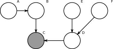
(a)

(b)

Figure 1: (a) An example directed graphical model on which we could use the KLC bound. Given the observed node C, the nodes A,F d-separate given nodes B,D,E. Thus we could make an explicit variational approximation for A,F, whilst marginalising B,D,E. Alternatively, we could select B,D,E for a parameterised approximate distribution, whilst marginalising A,F. (b) A sketch of the KLC and MF bounds. At the point where the mean field method has $q({\bf X})=q^{\star}({\bf X})$, the bounds are equal in value as well as in gradient. Away from the this point, the different between the bounds is the Kullback Leibler divergence between the current MF approximation for ${\bf X}$ and the implicit distribution $q^{\star}({\bf X})$ of the KLC bound.

4 Riemannian Gradient Based Optimisation

Sato (2001) and Hoffman et al. (2012) showed that the VBEM procedure performs gradient ascent in the space of the natural parameters. Using the KLC bound to collapse the problem, gradient methods seem a natural choice for optimisation, since there are fewer parameters to deal with, and we have shown that computation of the gradients is straightforward (the variational update equations contain the model gradients). It turns out that the KLC bound is particularly amenable to Riemannian or natural gradient methods, because the information geometry of the exponential family distrubution(s), over which we are optimising, leads to a simple expression for the natural gradient. Previous investigations of natural gradients for variational Bayes (Honkela et al., 2010; Kuusela et al., 2009) required the inversion of the Fisher information at every step (ours does not), and also used VBEM steps for some parameters and Riemannian optimisation for other variables. The collapsed nature of the KLC bound means that these VBEM steps are unnecessary: the bound can be computed by parameterizing the distribution of only one set of variables ($q({\bf Z})$) whilst the implicit distribution of the other variables is given in terms of the first distribution and the data by equation (5).

We optimize the lower bound $\mathcal{L}_{\text{KL}}$ with respect to the parameters of the approximating distribution of the non-collapsed variables. We showed in section 2 that the gradient of the KLC bound is given by the gradient of the standard MF variational bound, after an update of the collapsed variables. It is clear from their definition that the same is true of the natural gradients.

4.1 Variable Transformations

We can compute the natural gradient of our collapsed bound by considering the update equations of the non-collapsed problem as described above. However, if we wish to make use of more powerful optimisation methods like conjugate gradient ascent, it is helpful to re-parameterize the natural parameters in an unconstrained fashion. The natural gradient is given by (Amari and Nagaoka, 2007):

$$\widetilde{\bf g}({\boldsymbol{\theta}})=G({\boldsymbol{\theta}})^{-1}\frac{\partial\mathcal{L}_{\text{KL}}}{\partial{\boldsymbol{\theta}}}$$ (13)

where $G({\boldsymbol{\theta}})$ is the Fisher information matrix whose $i$,$j^{\text{th}}$ element is given by

$$G({\boldsymbol{\theta}})_{[i,j]}=-\mathbb{E}_{q({\bf X}\,|\,{\boldsymbol{\theta}})}\Big{[}{\frac{\partial^{2}\ln q({\bf X}\,|\,{\boldsymbol{\theta}})}{\partial{\boldsymbol{\theta}}^{[i]}\partial{\boldsymbol{\theta}}^{[j]}}}\Big{]}.$$ (14)

For exponential family distributions, this reduces to $\nabla^{2}_{\boldsymbol{\theta}}\psi({\boldsymbol{\theta}})$, where $\psi$ is the log-normaliser. Further, for exponential family distributions, the Fisher information in the canonical parameters $({\boldsymbol{\theta}})$ and that in the expectation parameters $({\boldsymbol{\eta}})$ are reciprocal, and we also have $G({\boldsymbol{\theta}})=\partial{\boldsymbol{\eta}}/\partial{\boldsymbol{\theta}}$. This means that the natural gradient in ${\boldsymbol{\theta}}$ is given by

$$\widetilde{\bf g}({\boldsymbol{\theta}})=G({\boldsymbol{\theta}})^{-1}\frac{\partial{\boldsymbol{\eta}}}{\partial{\boldsymbol{\theta}}}\frac{\partial\mathcal{L}_{\text{KL}}}{\partial{\boldsymbol{\eta}}}=\frac{\partial\mathcal{L}_{\text{KL}}}{\partial{\boldsymbol{\eta}}}\,\,\,\text{and}\,\,\,\widetilde{\bf g}({\boldsymbol{\eta}})=\frac{\partial\mathcal{L}_{\text{KL}}}{\partial{\boldsymbol{\theta}}}.$$ (15)

The gradient in one set of parameters provides the natural gradient in the other. Thus when our approximating distribution $q$ is exponential family, we can compute the natural gradient without the expensive matrix inverse.

4.2 Steepest Ascent is Coordinate Ascent

Sato (2001) showed that the VBEM algorithm was a gradient based algorithm. In fact, VBEM consists of taking unit steps in the direction of the natural gradient of the canonical parameters. From equation (9) and the work of Sato (2001), we see that the gradient of the KLC bound can be obtained by considering the standard mean-field update for the non-collapsed parameter ${\bf Z}$. We confirm these relationships for the models studied in the next section in the supplementary material.

Having confirmed that the VB-E step is equivalent to steepest-gradient ascent we now explore whether the procedure could be improved by the use of conjugate gradients.

4.3 Conjugate Gradient Optimization

One idea for solving some of the problems associated with steepest ascent is to ensure each gradient step is conjugate (geometrically) to the previous. Honkela et al. (2010) applied conjugate gradients to the standard mean field bound, we expect much faster convergence for the KLC bound due to its differing curvature. Since VBEM uses a step length of 1 to optimize, we also used this step length in conjugate gradients. In the natural conjugate gradient method, the search direction at the $i^{\text{th}}$ iteration is given by ${\bf s}_{i}=-\widetilde{\bf g}_{i}+\beta{\bf s}_{i-1}$. Empirically the Fletcher-Reeves method for estimating $\beta$ worked well for us:

$$\beta_{FR}=\frac{\langle\widetilde{\bf g}_{i},\widetilde{\bf g}_{i}\rangle_{i}}{\langle\widetilde{\bf g}_{i-1},\widetilde{\bf g}_{i-1}\rangle_{i-1}}\\$$ (16)

where $\langle\cdot,\cdot\rangle_{i}$ denotes the inner product in Riemannian geometry, which is given by $\widetilde{\bf g}^{\top}G(\rho)\widetilde{\bf g}$. We note from Kuusela et al. (2009) that this can be simplified since $\widetilde{\bf g}^{\top}G\widetilde{\bf g}=\widetilde{\bf g}^{\top}GG^{-1}{\bf g}=\widetilde{\bf g}^{\top}{\bf g}$, and other conjugate methods, defined in the supplementary material, can be applied similarly.

5 Experiments

For empirical investigation of the potential speed ups we selected a range of probabilistic models. We provide derivations of the bound and fuller explanations of the models in the supplementary material. In each experiment, the algorithm was considered to have converged when the change in the bound or the Riemannian gradient reached below $10^{-6}$. Comparisons between optimisation procedures always used the same initial conditions (or set of initial conditions) for each method. First we recreate the mixture of Gaussians example described by Honkela et al. (2010).

5.1 Mixtures of Gaussians

For a mixture of Gaussians, using the d-separation rule, we select for ${\bf X}$ the cluster allocation (latent) variables. These are parameterised through the softmax function for unconstrained optimisation. Our model includes a fully Bayesian treatment of the cluster parameters and the mixing proportions, whose approximate posterior distributions appear as (5). Full details of the algorithm derivation are given in the supplementary material. A neat feature is that we can make use of the discussion above to derive an expression for the natural gradient without a matrix inverse.

In Honkela et al. (2010) data are drawn from a mixture of five two-dimensional Gaussians with equal weights, each with unit spherical covariance. The centers of the components are at $(0,0)$ and $(\pm R,\pm R)$. $R$ is varied from $1$ (almost completely overlapping) to $5$ (completely separate). The model is initialised with eight components with an uninformative prior over the mixing proportions: the optimisation procedure is left to select an appropriate number of components.

Sung et al. (2008) reported that their collapsed method led to improved convergence over VBEM. Since our objective is identical, though our optimisation procedure different, we devised a metric for measuring the efficacy of our algorithms which also accounts for their propensity to fall into local minima. Using many randomised restarts, we measured the average number of iterations taken to reach the best-known optimum. If the algorithm converged at a lesser optimum, those iterations were included in the denomiator, but we didn’t increment the numerator when computing the average. We compared three different conjugate gradient approaches and standard VBEM (which is also steepest ascent on the KLC bound) using 500 restarts.

Table 1 shows the number of iterations required (on average) to come within 10 nats of the best known solution for three different conjugate-gradient methods and VBEM. VBEM sometimes failed to find the optimum in any of the 500 restarts. Even relaxing the stringency of our selection to 100 nats, the VBEM method was always at least twice as slow as the best conjugate method.

Table 1: Iterations to convergence for the mixture of Gaussians problem, with varying overlap (R). This table reports the average number of iterations taken to reach (within 10 nats of) the best known solution. For the more difficult scenarios (with more overlap in the clusters) the VBEM method failed to reach the optimum solution within 500 restarts

CG. method	$R=1$	$R=2$	$R=3$	$R=4$	$R=5$
Polack-Ribiére	$3,100.37$	$15,698.57$	$5,767.12$	$1,613.09$	$3,046.25$
Hestenes-Stiefel	$1,371.55$	$5,501.25$	$5,922.4$	$\mathbf{358.03}$	$\mathbf{172.39}$
Fletcher-Reeves	$\mathbf{416.18}$	$\mathbf{1,161.35}$	$\mathbf{5,091.0}$	$792.10$	$494.24$
VBEM	$\infty$	$\infty$	$\infty$	$992.07$	$429.57$

5.2 Topic Models

Latent Dirichlet allocation (LDA) (Blei et al., 2003) is a popular approach for extracting topics from documents. To demonstrate the KLC bound we applied it to 200 papers from the 2011 NIPS conference. The PDFs were preprocessed with pdftotext, removing non-alphabetical characters and coarsely filtering words by popularity to form a vocabulary size of 2000. We selected the latent topic-assignment variables for parameterisation, collapsing the topics and the document proportions. Conjugate gradient optimization was compared to the standard VBEM approach.

We used twelve random initializations, starting each algorithm from each initial condition. Topic and document distributions where treated with fixed, uninformative priors. On average, the Hestenes-Steifel algorithm was almost ten times as fast as standard VB, as shown in Table 2, whilst the final bound varied little between approaches.

Table 2: Time and iterations taken to run LDA on the NIPS 2011 corpus, $\pm$ one standard deviation, for two conjugate methods and VBEM. The Fletcher-Reeves conjugate algorithm is almost ten times as fast as VBEM. The value of the bound at the optimum was largely the same: deviations are likely just due to the choice of initialisations, of which we used 12.

Method	Time (minutes)	Iterations	Bound
Hestenes-Steifel	$56.4\pm 18.5$	$644.3\pm 214.5$	$-1,998,780\pm 201$
Fletcher-Reeves	$\mathbf{38.5\pm 8.7}$	$\mathbf{447.8\pm 100.5}$	$-1,998,743\pm 194$
VBEM	$370\pm 105$	$4,459\pm 1,296$	$-1,998,732\pm 241$

5.3 RNA-seq alignment

An emerging problem in computational biology is inference of transcript structure and expression levels using next-generation sequencing technology (RNA-Seq). Several models have been proposed. The BitSeq method (Glaus et al., 2012) is based on a probabilistic model and uses Gibbs sampling for approximate inference. The sampler can suffer from particularly slow convergence due to the large size of the problem, which has six million latent variables for the data considered here. We implemented a variational version of their model and optimised it using VBEM and our collapsed Riemannian method. We applied the model to data described in Xu et al. (2010), a study of human microRNA. The model was initialised using four random initial conditions, and optimised using standard VBEM and the conjugate gradient versions of the algorithm. The Polack-Ribiére conjugate method performed very poorly for this problem, often giving negative conjugation: we omit it here. The solutions found for the other algorithms were all fairly close, with bounds coming within 60 nats. The VBEM method was dramatically outperformed by the Fletcher-Reeves and Hestenes-Steifel methods: it took $4600\pm 20$ iterations to converge, whilst the conjugate methods took only $268\pm 4$ and $265\pm 1$ iterations to converge. At about 8 seconds per iteration, our collapsed Riemannian method requires around forty minutes, whilst VBEM takes almost eleven hours. All the variational approaches represent an improvement over a Gibbs sampler, which takes approximately one week to run for this data (Glaus et al., 2012).

6 Discussion

Under very general conditions (conjugate exponential family) we have shown the equivalence of collapsed variational bounds and marginalized variational bounds using the KL corrected perspective of King and Lawrence (2006). We have provided a succinct derivation of these bounds, unifying several strands of work and laying the foundations for much wider application of this approach.

When the collapsed variables are updated in the standard MF bound the KLC bound is identical to the MF bound in value and gradient. Sato (2001) has shown that coordinate ascent of the MF bound (as proscribed by VBEM updates) is equivalent to steepest ascent of the MF bound using natural gradients. This implies that standard variational inference is also performing steepest ascent on the KLC bound. This equivalence between natural gradients and the VBEM update equations means our method is quickly implementable for any model where the mean field update equations have been computed. It is only necessary to determine which variables to collapse using a d-separation test. Importantly this implies our approach can readily be incorporated in automated inference engines such as that provided by infer.net (Minka et al., 2010). We’d like to emphasise the ease with which the method can be applied: we have provided derivations of equivalencies of the bounds and gradients which should enable collapsed conjugate optimisation of any existing mean field algorithm, with minimal changes to the software. Indeed our own implementations (see supplementary material) use just a few lines of code to switch between the VBEM and conjugate methods.

The improved performance arises from the curvature of the KLC bound. We have shown that it is always less negative than that of the original variational bound allowing much larger steps in the variational parameters as King and Lawrence (2006) suggested. This also provides a gateway to second-order optimisation, which could prove even faster.

We provided empirical evidence of the performance increases that are possible using our method in three models. In a thorough exploration of the convergence properties of a mixture of Gaussians model, we concluded that a conjugate Riemannian algorithm can find solutions that are not found with standard VBEM. In a large LDA model, we found that performance can be improved many times over that of the VBEM method. In the BitSeq model for differential expression of genes transcripts we showed that very large improvements in performance are possible for models with huge numbers of latent variables.

Supplementary Material for:
Fast Variational Inference
in the Conjugate Exponential Family

This supplementary material accompanies the NIPS paper on Fast Variational Inference in the Conjugate Exponential Family. Its purpose is to provide details of how our very general framework applies in the case of the specific models described in the paper. First we briefly mention the form of the three conjugate gradient algorithms we used in optimization.

7 Conjugate gradient algorithms

There are several different methods for approximating the parameter $\beta$ in the conjugate gradient algorithm. We used the Polack-Ribière, Fletch-Reeves or Hestenes-Stiefel methods:

$$\begin{split}\beta_{PR}=\frac{\langle\widetilde{\bf g}_{i},\widetilde{\bf g}_{i}-\widetilde{\bf g}_{i-1}\rangle_{i}}{\langle\widetilde{\bf g}_{i-1},\widetilde{\bf g}_{i-1}\rangle_{i-1}}\\ \beta_{FR}=\frac{\langle\widetilde{\bf g}_{i},\widetilde{\bf g}_{i}\rangle_{i}}{\langle\widetilde{\bf g}_{i-1},\widetilde{\bf g}_{i-1}\rangle_{i-1}}\\ \beta_{HS}=\frac{\langle\widetilde{\bf g}_{i},\widetilde{\bf g}_{i}-\widetilde{\bf g}_{i-1}\rangle_{i}}{\langle\widetilde{\bf g}_{i-1},\widetilde{\bf g}_{i}-\widetilde{\bf g}_{i-1}\rangle_{i-1}}\end{split}$$ (17)

where $\langle\cdot,\cdot\rangle_{i}$ denotes the inner product in Riemannian geometry, which is given by $\widetilde{\bf g}^{\top}G(\rho)\widetilde{\bf g}$

8 Mixture of Gaussians

A MoG model is defined as follows. We have a set of $N$ $D$-dimensional vectors ${\bf Y}=\{{\bf y}_{n}\}_{n=1}^{N}$. The likelihood is

$$p({\bf Y}|{\boldsymbol{\eta}},{\bf L})=\prod_{k=1}^{K}\prod_{n=1}^{N}\mathcal{N}({\bf y}_{n}|{\boldsymbol{\mu}}_{k},{\boldsymbol{\Lambda}}_{k}^{-1})^{\ell_{nk}}$$ (18)

where ${\bf L}$ is a collection of binary latent variables indicating cluster membership, ${\bf L}=\{\{\boldsymbol{\ell}_{nk}\}_{n=1}^{N}\}_{k=1}^{K}$ and ${\boldsymbol{\eta}}$ is a collection of cluster parameters, ${\boldsymbol{\eta}}=\{{\boldsymbol{\mu}}_{k},{\boldsymbol{\Lambda}}_{k}\}_{k=1}^{K}$

The prior over ${\bf L}$ is given by a multinomial distribution with components ${\boldsymbol{\pi}}$, which in turn have a Dirichlet prior with uniform concentrations for simplicity:

$$p({\bf L}|{\boldsymbol{\pi}})=\prod_{k=1}^{K}\prod_{n=1}^{N}\pi_{k}^{\ell_{nk}},\hskip 12.23447ptp({\boldsymbol{\pi}})=R_{D}({\boldsymbol{\alpha}})\prod_{k=1}^{K}\pi_{k}^{\alpha-1}$$ (19)

with ${\boldsymbol{\alpha}}$ representing a $K$ dimensional vector with elements $\alpha$, and $R_{D}$ being the normalising constant for the Dirichlet distribution, $R_{D}({\boldsymbol{\alpha}})=\Gamma(K\alpha)\Gamma(\alpha)^{-K}$.

Finally we choose a conjugate Gaussian-Wishart prior for the cluster parameters which can be written

$$\begin{split}\ln p({\boldsymbol{\mu}}_{k},{\boldsymbol{\Lambda}}_{k})=\ln R_{GW}({\bf S}_{0},\nu_{0},\kappa_{0})+\frac{\nu_{0}-D}{2}\ln|{\boldsymbol{\Lambda}}_{k}|\\ -\frac{1}{2}\text{tr}\left({\boldsymbol{\Lambda}}_{k}\left(\kappa_{0}{\boldsymbol{\mu}}_{k}{\boldsymbol{\mu}}_{k}^{\top}+\kappa_{0}{\bf m}_{0}{\bf m}_{0}^{\top}-2\kappa_{0}{\bf m}_{0}{\boldsymbol{\mu}}_{k}^{\top}+{\bf S}_{0}\right)\right)\end{split}$$ (20)

where $R_{GW}$ is the normalising constant, and is given by

$$R_{GW}({\bf S},\nu,\kappa)=|{\bf S}|^{\frac{\nu}{2}}2^{-\frac{(\nu+1)D}{2}}\pi^{-\frac{D(D+1)}{4}}\kappa^{\frac{D}{2}}(\prod_{d=1}^{D}\Gamma((\nu+1-d)/2))^{-1}.$$

8.1 Applying the KLC bound

The first task in applying the KLC bound is to select which variables to parameterise and which to marginalise. From the graphical model representation of the MoG problem in Figure 2, we can see that we can select the latent variables ${\bf Z}=\{{\bf L}\}$ for parameterisation, whilst marginalising the mixing proportions and cluster parameters (${\bf X}=\{{\boldsymbol{\pi}},{\boldsymbol{\eta}}\}$). We note that it is possible to select the variables the other way around: parameterising ${\boldsymbol{\pi}}$ and ${\boldsymbol{\eta}}$ and marginalising ${\bf L}$, but parameterisation of the latent variables makes implementation a little simpler.

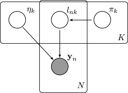
Figure 2: A graphical model representation of the MoG model. A d-separation test quickly shows that it is possible to marginalise ${\boldsymbol{\pi}}$ and ${\boldsymbol{\eta}}$ given a variational parameterisation of ${\bf L}$.

We use a factorised multinomial distribution $q({\bf L})$ to approximate the posterior for $p({\bf L}|{\bf Y})$, parameterised using the softmax functions so

$$q({\bf L})=\prod_{n=1}^{N}\prod_{k=1}^{K}r_{nk}^{\boldsymbol{\ell}_{nk}}\,\,,\,\,\,\,\,r_{nk}=\frac{e^{\rho_{nk}}}{\sum_{i=1}^{K}e^{\rho_{ni}}}.$$ (21)

We are now ready to apply the procedure described above to derive the KLC bound. First,

$$\ln p({\bf Y}|{\boldsymbol{\eta}},{\boldsymbol{\pi}})\geq\int\!q({\bf L})\{\ln p({\bf Y}|{\boldsymbol{\eta}},{\bf L})+\ln p({\bf L}|{\boldsymbol{\pi}})\}\,\text{d}{\bf L}+H_{L},$$ (22)

where $H_{L}$ is the entropy of the distribution $q({\bf L})$. We expand to give

$$\begin{split}\mathcal{L}_{1}=\tfrac{1}{2}\sum_{k=1}^{K}\Big{\{}-\text{tr}\big{(}{\boldsymbol{\Lambda}}_{k}\big{(}\widehat{r}_{k}{\boldsymbol{\mu}}_{k}{\boldsymbol{\mu}}_{k}^{\top}+C_{k}-2{\boldsymbol{\mu}}_{k}\bar{\bf y}_{k}\big{)}\big{)}\\ +\widehat{r}_{k}\ln\pi_{k}+\widehat{r}_{k}\ln|{\boldsymbol{\Lambda}}_{k}|\Big{\}}+H_{L}-\tfrac{ND}{2}\ln(2\pi)\end{split}$$ (23)

where $\widehat{r}_{k}=\sum_{n=1}^{N}r_{nk}$, $C_{k}=\sum_{n=1}^{N}r_{nk}{\bf y}_{n}{\bf y}_{n}^{\top}$, and $\bar{\bf y}_{k}=\sum_{n=1}^{N}r_{nk}{\bf y}_{n}$. The conjugacy between the intermediate bound $\mathcal{L}_{1}$ and the prior now emerges, making the second integral in the KLC bound tractable.

After exponentiating this expression and multiplying by the prior, $p({\boldsymbol{\eta}})p({\boldsymbol{\pi}})$, we find that the integrals with respect to both ${\boldsymbol{\eta}}$ and ${\boldsymbol{\pi}}$ are tractable. This result means that the only variational parameters needed are those of $q({\bf L})$. The integrals result in

$$\begin{split}\mathcal{L}_{\text{KL}}=-\frac{ND}{2}\ln(2\pi)+\ln R_{Di}({\boldsymbol{\alpha}})-\ln R_{Di}({\boldsymbol{\alpha}}^{\prime})\\ +K\ln R_{GW}({\bf S}_{0},\nu_{0},\kappa_{0})-\sum_{k=1}^{K}\ln R_{GW}({\bf S}_{k},\nu_{k},\kappa_{k})+H_{L}\end{split}$$ (24)

where we have defined

$$\begin{split}\alpha_{k}&=\alpha+\widehat{r}_{k}\hskip 71.13188pt\kappa_{k}=\kappa_{0}+\widehat{r}_{k}\\ {\bf m}_{k}&=(\kappa_{0}{\bf m}_{0}+\bar{\bf y}_{k})/\kappa_{k}\hskip 28.45274pt\nu_{k}=\nu_{0}+\widehat{r}_{k}\\ {\bf S}_{k}&=S_{0}+C_{k}+\kappa_{0}{\bf m}_{0}{\bf m}_{0}^{\top}-\kappa_{k}{\bf m}_{k}{\bf m}_{k}^{\top}\end{split}$$ (25)

and ${\boldsymbol{\alpha}}^{\prime}$ represents a vector containing each $\alpha_{k}$. Some simplification of (24) leads to

$$\begin{split}\mathcal{L}_{\text{KL}}&=\sum_{k=1}^{K}\Big{\{}\ln\Gamma(\alpha_{k})-\tfrac{D}{2}\ln\kappa_{k}-\tfrac{\nu_{k}}{2}\ln|S_{k}|\\ &+\sum_{d=1}^{D}\ln\Gamma((\nu_{k}+1-d)/2)\Big{\}}+H_{L}+\text{const.}\end{split}$$ (26)

where const. contains terms independent of ${\bf r}$.

Equations (25) are similar to the update equations for the approximating distributions in the VBEM methodology [see e.g. Bishop, 2006]. However, for our model they are simply intermediate variables, representing combinations of the true variational parameters ${\bf r}$, the data, and the model prior parameters. When optimizing the model with respect to the variational parameters, the dependency of these intermediate variables on ${\bf r}$ is not ignored as it would be in MF variational approach.

The gradient of the MV bound (26) with respect to the parameters ${\bf r}$ is given by

$$\begin{split}\frac{\partial\mathcal{L}_{\text{KL}}}{\partial r_{nk}}=&-\tfrac{D}{2}\kappa_{k}^{-1}-\tfrac{1}{2}\ln|S_{k}|+\psi(\alpha_{k})-\ln r_{nk}\\ &-\tfrac{\nu_{k}}{2}(y_{n}-{\bf m}_{k})^{\top}S_{k}^{-1}(y_{n}-{\bf m}_{k}))\\ &+\tfrac{1}{2}\sum_{d=1}^{D}\psi((\nu_{k}+1-d)/2)-1.\end{split}$$ (27)

Taking a step in this direction (in the valiables $\gamma$) yields exactly the VB-E step associated with the mean-field bound. the gradient in $r$ is the natural gradient in $\gamma$ (see paper section 4.1).

9 Latent Dirichlet Allocation

Latent Dirichlet allocation is a popular topic model. See Blei et al. [2003] for a thorough introduction.

Suppose we have $D$ documents, $K$ topics and a vocabulary of size $V$. The $d^{\text{th}}$ document contains $N_{d}$ words $W_{d}=\{w_{dn}\}_{n=1}^{N_{d}}$, and each word is represented as a binary vector $w_{dn}\in\{0,1\}^{V}$. Each word is associated with a latent variable $\boldsymbol{\ell}_{dn}$, which assigns the word to a topic, thus $\boldsymbol{\ell}_{dn}\in\{0,1\}^{K}$. We’ll use $W$ to represent the colletion of all words, $W=\{W_{d}\}_{d=1}^{D}$, and ${\bf L}$ to represent the collection of all latent variables ${\bf L}=\{\{\boldsymbol{\ell}_{dn}\}_{n=1}^{N_{d}}\}_{d=1}^{D}$.

Each document has an associated vector of topic proportions, $\theta_{d}\in[0,1]^{K}$, and each topic is represented by a vector of word proportions $\phi_{k}\in[0,1]^{V}$. We assume a symmetrical prior distribution over topics in each document $p(\theta_{d})=\textit{Dir}(\theta_{d}|\alpha)$, and similarly for words within topics. $p(\phi_{k})=\textit{Dir}(\phi_{k}|\beta)$.

The LDA generative model states that for each word, first the associated topic is drawn from the topic proportions for the document, and then the word is drawn from the selected topic.

$$\begin{split}p(\ell_{dn}|\theta_{d})&=\prod_{k=1}^{K}\theta_{dk}^{\boldsymbol{\ell}_{dnk}}\\ p(w_{dn}|\boldsymbol{\ell}_{dn},\phi)&=\prod_{k=1}^{K}\prod_{v=1}^{V}\phi_{kv}^{w_{dnv}\boldsymbol{\ell}_{dnk}}\\ \end{split}$$ (28)

9.1 The collapsed bound

To derive the colapsed bound, we use a similar d-separation test as for the mixture model to select the latent variables as the parameteriser (non-collapsed) nodes. See Figure 3.

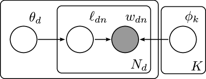
Figure 3: A graphical model representation of Latent Dirichlet allocation. A d-separation test quickly shows that it is possible to marginalise $\theta$ and $\phi$ given a variational parameterisation of ${\bf L}$.

To proceed we assume a factorising multinomial posterior for ${\bf L}$:

$$q({\bf L})=\prod_{d=1}^{D}\prod_{n=1}^{N_{d}}\prod_{k=1}^{K}r_{dnk}^{\boldsymbol{\ell}_{dnk}}$$ (29)

subject to the constraint $\sum_{k=1}^{K}\boldsymbol{\ell}_{dnk}=1$, which we enforce through a softmax reparameterisation

$$r_{dnk}=\frac{e^{\rho_{dnk}}}{\sum_{k^{\prime}=1}^{K}e^{\rho_{dnk^{\prime}}}}.$$ (30)

We proceed by deriving the conditional bound

$$\ln p(W\,|\,\theta,\phi)\geq\mathcal{L}_{1}=\sum_{d=1}^{D}\sum_{n=1}^{N_{d}}\sum_{k=1}^{K}\sum_{v=1}^{V}(w_{dnv}r_{dnk})\ln\phi_{kv}+\sum_{d=1}^{D}\sum_{n=1}^{N_{d}}\sum_{k=1}^{K}(r_{dnk}\ln\theta_{dk})+H[q({\bf L})].$$ (31)

To marginalise the variables $\theta,\phi$, we exponentiate this bound and take the expectation under the priors. This results in

$$\begin{split}p(W)\geq\int\!\exp\{\mathcal{L}_{1}\}p(\theta)p(\phi)\,\text{d}\theta\,\text{d}\phi=&\int\!\prod_{k=1}^{K}\prod_{v=1}^{V}\phi_{kv}^{\sum_{d=1}^{d}\sum_{n=1}^{n_{d}}(w_{dnv}r_{dnk})}\prod_{d=1}^{D}\prod_{k=1}^{K}\theta_{dk}^{(\sum_{n=1}^{N_{d}}r_{dnk})}\\ &\prod_{k=1}^{K}R_{Di}(\beta)\prod_{v=1}^{V}\phi_{kv}^{\beta-1}\\ &\prod_{d=1}^{D}R_{Di}(\alpha)\prod_{k=1}^{K}\theta_{dk}^{\alpha-1}\,\text{d}\theta\,\text{d}\phi\\ &\exp\{H[q({\bf L})]\}.\end{split}$$ (32)

Careful inspection of the above reveals that the two integrals separate as expected, and result in the normalizers for each of the independent Dirichlet approximations. Taking the logarithm reults in

$$\mathcal{L}_{\text{KL}}=D\ln R_{Di}(\alpha)-\sum_{d=1}^{D}\ln R_{Di}(\alpha_{d}^{\prime})+K\ln R_{Di}(\beta)-\sum_{k=1}^{K}\ln R_{Di}(\beta_{k}^{\prime})+H[q({\bf L})]$$ (33)

where we have defined $\alpha_{dk}^{\prime}=\alpha+\sum_{n=1}^{N_{d}}r_{dnk}$ and $\beta_{kv}^{\prime}=\beta+\sum_{d=1}^{d}\sum_{n=1}^{n_{d}}w_{dnv}r_{dnk}$.

9.2 Topics found by LDA

For completeness we show here some topics found by LDA on the NIPS conference data.

Table 3: some topics found using LDA on papers from the 2011 NIPS conference.

neural	training	distribution	data	features	model
input	feature	gaussian	points	image	models
neurons	classification	inference	point	object	variables
network	class	process	clustering	images	parameters
fig	tree	prior	distance	objects	structure
estimate	prediction	sampling	dataset	scene	variable
neuron	label	likelihood	similarity	recognition	markov
visual	accuracy	posterior	cluster	reference	observed
nonlinear	labels	distributions	manifold	detection	graphical
linear	classifier	bayesian	spectral	part	hidden

10 BitSeq Model

The generative model for an RNA-seq assay is as follows. We assume that the experiment consists of a pile of RNA fragments, where the abundance of fragments from transcript $T_{m}$ in the assay is $\theta_{m}$. The sequencer then selects a fragment at random from the pile, such that the probability of picking a fragment corresponding to transcript $T_{m}$ is $\theta_{m}$. Introducing a convenient membership vector $\boldsymbol{\ell}_{n}$ for each read, we can write

$$p({\bf L}|{\boldsymbol{\theta}})=\prod_{n=1}^{{N}}\prod_{m=1}^{{M}}\theta_{m}^{\boldsymbol{\ell}_{nm}}$$ (34)

where $\ell_{nm}\in\{0,1\}$ is a binary variable which indicates whether the $n$th fragment came from the $m$th transcript ($\ell_{nm}=1$) and is subject to $\sum_{m=1}^{{M}}\ell_{nm}=1$. We use ${\bf L}$ to represent the collection of all alignment variables.

Both $\theta$ and ${\bf L}$ are variables to be inferred, with ${\boldsymbol{\theta}}$ the main object of interest.

Writing the collection of all reads as $\mathbf{R}=\{{\bf r}_{n}\}_{n=1}^{N}$, the likelihood of a set of alignments ${\bf L}$ is

$$p(\mathbf{R}|\mathbf{T},{\bf L})=\prod_{n=1}^{{N}}p({\bf r}_{n}|T_{m})^{\ell{nm}}$$ (35)

where $T_{m}$ represents the $m$th transcript, $\mathbf{T}$ represents the transcriptome.

The values of $p(r_{n}|T_{m})$ can be computed before performing inference in ${\boldsymbol{\theta}}$ since we are assuming a known transcriptome. We compute these values based on the quality of alignment of the read ${\bf r}_{n}$ to the transcript $T_{m}$, using a model which can correct for sequence specific or fragmentation biases. The method is described in detatil in Glaus et al. [2012].

We specify a conjugate Dirichlet prior over the vector ${\boldsymbol{\theta}}$.

$$p({\boldsymbol{\theta}})=\frac{\Gamma(\hat{\alpha}^{o})}{\prod_{m=1}^{{M}}\Gamma(\alpha^{o}_{m})}\prod_{m=1}^{{M}}\theta_{m}^{\alpha^{o}_{m}-1}$$ (36)

with $\hat{\alpha}^{o}=\sum_{m=1}^{{M}}\alpha^{o}_{m}$. $\alpha^{o}_{m}$ represents our prior belief in the values of $\theta_{m}$, and we use a relatively uninformative but proper prior $\alpha^{o}_{m}=1\,\forall m=1\ldots M$. A priori, we assume that the concentrations are all equal, but with large uncertainty.

10.1 The collapsed bound

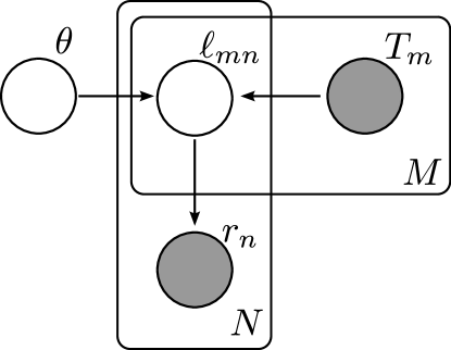
Figure 4: A graphical model representation of the BitSeq model. A d-separation test quickly shows that it is possible to marginalise $\theta$ given a variational parameterisation of ${\bf L}$.

Figure 4 shows a graphical representation of the BitSeq model. It’s clear that parameterisation of the latent variables will allow us to collapse $\theta$, or vica-versa. Selecting again the latent variables for parameterisation, ${\bf X}=\{{\bf L}\}$, ${\bf Z}=\{\theta\}$, we first find the conditional bound as usual by:

$$\begin{split}\ln p(\mathbf{R}\,|\,\mathbf{T},{\boldsymbol{\theta}})&=\ln\int\!p(\mathbf{R}\,|\,{\bf L},\mathbf{T})p({\bf L}\,|\,{\boldsymbol{\theta}})\,\text{d}{\bf L}\\ &\geq\mathbb{E}_{q({\bf L})}\Big{[}{\ln p(\mathbf{R}\,|\,{\bf L},\mathbf{T})+\ln p({\bf L}\,|\,{\boldsymbol{\theta}})-\ln q({\bf L})}\Big{]}\\ &\geq\sum_{n=1}^{{N}}\sum_{m=1}^{{M}}\ell_{nm}\big{(}\ln p({\bf r}_{n}\,|\,T_{m})+\ln\theta_{m}-\ln\ell_{nm}\big{)}\\ &\geq\mathcal{L}_{1}\end{split}$$ (37)

It’s clear that this bound is conjugate to the prior for $\theta$, so we can marginalise:

$$\begin{split}\ln p(\mathbf{R}\,|\,\mathbf{T})\geq\mathcal{L}_{\text{KL}}=\sum_{n=1}^{{N}}\sum_{m=1}^{{M}}\ell_{nm}\big{(}\ln p({\bf r}_{n}\,|\,T_{m})-\ln\ell_{nm}\big{)}+\ln\Gamma(\hat{\alpha}^{o})-\ln\Gamma(\hat{\alpha}^{o}+N)\\ -\sum_{m=1}^{{M}}\Big{(}\ln\Gamma(\alpha^{o}_{m})-\ln\Gamma(\alpha^{o}_{m}+\hat{\ell}_{m})\Big{)}\end{split}$$ (38)

where $\hat{\ell}_{m}=\sum_{n=1}^{{N}}\ell_{n}$ and we also have that the approximate posterior distribution for ${\boldsymbol{\theta}}$ is a Dirichlet distribution with parameters $\alpha^{o}_{m}+\hat{\ell}_{m}$.

References

- Amari and Nagaoka [2007] S. Amari and H. Nagaoka. Methods of information geometry. AMS, 2007.
- Asuncion et al. [2012] A. Asuncion, M. Welling, P. Smyth, and Y. Teh. On smoothing and inference for topic models. arXiv preprint arXiv:1205.2662, 2012.
- Bishop [2006] C. M. Bishop. Pattern Recognition and Machine Learning. Springer New York, 2006.
- Blei et al. [2003] D. M. Blei, A. Y. Ng, and M. I. Jordan. Latent Dirichlet allocation. The Journal of Machine Learning Research, 3:993–1022, 2003.
- Glaus et al. [2012] P. Glaus, A. Honkela, and M. Rattray. Identifying differentially expressed transcripts from RNA-seq data with biological variation. Bioinformatics, 2012. doi: 10.1093/bioinformatics/bts260. Advance Access.
- Hoffman et al. [2012] M. Hoffman, D. Blei, C. Wang, and J. Paisley. Stochastic variational inference. arXiv preprint arXiv:1206.7051, 2012.
- Honkela et al. [2010] A. Honkela, T. Raiko, M. Kuusela, M. Tornio, and J. Karhunen. Approximate Riemannian conjugate gradient learning for fixed-form variational Bayes. The Journal of Machine Learning Research, 9999:3235–3268, 2010.
- King and Lawrence [2006] N. King and N. D. Lawrence. Fast variational inference for Gaussian process models through KL-correction. Machine Learning: ECML 2006, pages 270–281, 2006.
- Kurihara et al. [2007] K. Kurihara, M. Welling, and Y. W. Teh. Collapsed variational Dirichlet process mixture models. In Proceedings of the International Joint Conference on Artificial Intelligence, volume 20, page 19, 2007.
- Kuusela et al. [2009] M. Kuusela, T. Raiko, A. Honkela, and J. Karhunen. A gradient-based algorithm competitive with variational Bayesian EM for mixture of Gaussians. In Neural Networks, 2009. IJCNN 2009. International Joint Conference on, pages 1688–1695. IEEE, 2009.
- Lázaro-Gredilla and Titsias [2011] M. Lázaro-Gredilla and M. K. Titsias. Variational heteroscedastic Gaussian process regression. In Proceedings of the International Conference on Machine Learning (ICML), 2011, 2011.
- Lázaro-Gredilla et al. [2011] M. Lázaro-Gredilla, S. Van Vaerenbergh, and N. Lawrence. Overlapping mixtures of Gaussian processes for the data association problem. Pattern Recognition, 2011.
- Minka et al. [2010] T. P. Minka, J. M. Winn, J. P. Guiver, and D. A. Knowles. Infer .NET 2.4. Microsoft Research Cambridge, 2010.
- Sato [2001] M. A. Sato. Online model selection based on the variational Bayes. Neural Computation, 13(7):1649–1681, 2001.
- Sung et al. [2008] J. Sung, Z. Ghahramani, and S. Bang. Latent-space variational Bayes. Pattern Analysis and Machine Intelligence, IEEE Transactions on, 30(12):2236–2242, 2008.
- Teh et al. [2007] Y. W. Teh, D. Newman, and M. Welling. A collapsed variational Bayesian inference algorithm for latent Dirichlet allocation. Advances in neural information processing systems, 19:1353, 2007.
- Xu et al. [2010] G. Xu et al. Transcriptome and targetome analysis in MIR155 expressing cells using RNA-seq. RNA, pages 1610–1622, June 2010. ISSN 1355-8382. doi: 10.1261/rna.2194910. URL http://rnajournal.cshlp.org/cgi/doi/10.1261/rna.2194910.