Quantifying short-range correlations in nuclei

Abstract

Background

Short-range correlations (SRC) are an important ingredient of the dynamics of nuclei.

Purpose

An approximate method to quantify the magnitude of the two-nucleon (2N) and three-nucleon (3N) short-range correlations (SRC) and their mass dependence is proposed.

Method

The proposed method relies on the concept of the “universality” or “local nuclear character” of the SRC. We quantify the SRC by computing the number of independent-particle model (IPM) nucleon pairs and triples which reveal beyond-mean-field behavior. It is argued that those can be identified by counting the number of nucleon pairs and triples in a zero relative orbital momentum state. A method to determine the quantum numbers of pairs and triples in an arbitrary mean-field basis is outlined.

Results

The mass dependence of the 2N and 3N SRC is studied. The predictions are compared to measurements. This includes the ratio of the inclusive inelastic electron scattering cross sections of nuclei to ²H and ³He at large values of the Bjorken variable. Corrections stemming from the center-of-mass motion of the pairs are estimated.

Conclusions

We find that the relative probability per nucleon for 2N and 3N SRC has a soft dependence with mass number $A$ and that the proton-neutron 2N SRC outnumber the proton-proton (neutron-neutron) 2N SRC. A linear relationship between the magnitude of the EMC effect and the predicted number of proton-neutron SRC pairs is observed. This provides support for the role of local nuclear dynamics on the EMC effect.

I Introduction

We define the nuclear packing factor (NPF) as the fraction of the nuclear volume that is occupied by nucleons. A rough order of magnitude estimate of the NPF can be arrived at using uniform spheres for the nuclear and nucleon density. The nuclear radius $R_{A}$ can be reasonably determined from $R_{A}=1.2$(fm) $A^{1/3}$. It is not obvious what value of the nucleon radius $r_{N}$ should be used. In models of relativistic heavy-ion collisions it is customary Broniowski and Rybczynski (2010) to use expulsion distances $d$, which simulate the hard-core NN repulsion, of the order of 1 fm, corresponding with $r_{N}\approx$0.5 fm. This leads to NPF=0.07. A recent reanalysis of electron scattering data resulted in a root-mean-square charge radius of the proton $r_{p}^{c}=\sqrt{\left<r_{p}^{2}\right>}$=0.897(18) fm Blunden and Sick (2005). Assuming that the $r_{p}^{c}$ is an estimate of the proton and neutron radius one arrives at NPF= $\left(\frac{r_{p}^{c}\textrm{(fm)}}{1.2}\right)^{3}$=0.42. It is clear that the computed NPF is very sensitive to the adopted value of the nucleon radius. The estimate of the NPF on the basis of $r_{p}^{c}$ should be considered as an upper limit. Indeed, the established value of the nuclear saturation density of 0.17 nucleons/fm^³ corresponds with a mean internucleon distance of 1.8 fm implying that $r_{N}\leq 0.9$ fm.

From the above, it is clear that one expects that the nucleus is more like a saturated quantum liquid than a gas of freely moving nucleons. Accordingly, the nuclear wave functions receive large corrections from short-range (SRC) and long-range correlations. These days it is common practice to implement the effect of SRC in nuclear computations. Examples include the calculations of matrix elements for double-$\beta$ decay Engel et al. (2011), of event simulations in heavy-ion collisions Alvioli and Strikman (2011), and of hadron transparencies in nuclei Cosyn et al. (2008).

The EMC effect Aubert et al. (1983) is the reduction of the cross section for leptonic scattering off a nucleon bound in a nucleus relative to that of a free nucleon (mass $M_{N}$). The EMC effect was observed in Deep Inelastic Scattering (DIS) experiments on nuclei at high virtual-photon virtualities $Q^{2}=q^{2}-\omega^{2}\gtrsim 2$ GeV² for Bjorken $x_{B}=\frac{Q^{2}}{2M_{N}\omega}$ in the range $0.3\leq x_{B}\leq 0.7$. The ratio of per nucleon cross sections is denoted by $R=\frac{2}{A}\frac{\sigma^{A}}{\sigma^{D}}$ where $\sigma^{A}$ is the cross section for leptonic scattering from the target $A$. The magnitude of the EMC effect can be quantified by means of the slope $-\frac{dR}{dx_{B}}$ Seely et al. (2009). Another remarkable feature of the ratio $R$ is that it adopts a constant value (this factor is commonly referred to as the SRC scaling factor $a_{2}(A/D)$) for $1.5\lesssim x_{B}\lesssim 2$ and moderate values of $Q^{2}$ Day et al. (1987); Egiyan et al. (2006); Fomin et al. (2012). It has been suggested Frankfurt et al. (2008) that the $a_{2}(A/D)$ can be related to the high-momentum components of the nuclear wave functions. A phenomenological linear relationship between the $a_{2}(A/D)$ and the magnitude of the EMC effect expressed as $-\frac{dR}{dx_{B}}$ has been observed Weinstein et al. (2011); Hen et al. (2012); Arrington et al. (2012a). This indicates that the magnitude of the European Muon Collaboration (EMC) effect may be driven by SRC. In this picture the magnitude of the EMC effect is (partly) related to the temporal local density fluctuations which are induced by the high virtualities of the leptonic probe. Recent measurements Seely et al. (2009) corroborate this relation between the local nuclear environment and the magnitude of the EMC effect.

Given an arbitrary nucleus $A(N,Z)$ we address the issue of quantifying the number of two-nucleon (2N) pairs prone to SRC and the number of 3N triples prone to SRC. Along the same lines we investigate to what extent the mass dependence of the NN SRC can be captured by some approximate principles. We wish to develop a robust method which is applicable to any nucleus from He to Pb. From this method we expect, for example, that it allows one to study the mass dependence of the SRC without combining results from various types of calculations.

Momentum distributions contain the information about 1N, 2N, 3N, $\ldots$ properties of the nuclear ground state. Over the years various methods to compute the nuclear 1N and 2N momentum distributions have been developed. Ab-initio calculations which solve the Schrödinger equation with realistic nucleon-nucleon interactions are available for light nuclei like ⁴He Schiavilla et al. (2007); Wiringa et al. (2008); Feldmeier et al. (2011). For medium-weight nuclei (12 $\leq$ A $\leq$ 40) truncation schemes based on cluster expansions can be adopted Alvioli et al. (2008). Correlated-basis function theory has been applied to compute ground-state densities and momentum distributions for doubly-closed-shell nuclei from ¹²C to ²⁰⁸Pb Bisconti et al. (2006, 2007). Thanks to the enormous progress in theoretical many-body nuclear physics and the availability of nuclear momentum distributions in a broad mass range, times are ripe to learn more about SRC, for example by mapping its $A$ and isospin dependence. It remains notoriously difficult, though, to establish quantitative relationships between observables and the computed momentum distributions Frankfurt et al. (2008); Vanhalst et al. (2011); Arrington et al. (2012b); Shneor et al. (2007); Ryckebusch (2001, 1996). Here, we do not attempt a high-precision calculation of momentum distributions. Our goal is to gather insight into the mass and isospin dependence of the SRC from stylized facts of momentum distributions.

In a mean-field model fluctuations are completely ignored. The SRC induce spatio-temporal fluctuations from the mean-field predictions for the nuclear density distributions for example. As a result of SRC, realistic nuclear wave functions reflect the coexistence of single nucleon (mean-field) structures and cluster structures. The clusters account for beyond mean-field behavior. As the nucleon-nucleon interaction is short ranged, the clusters attributed to SRC are predominantly 2N. The central result of this paper asserts that the amount of 2N and 3N SRC in nuclei can be reasonably quantified by counting the number of nucleon pairs and triples in a zero relative orbital state in a mean-field ground-state wave function. In order to quantify the isospin dependence of the 2N and 3N correlations, additional information about the spin dependence of the clusters is necessary.

This paper is organized as follows. Sect. II is devoted to a discussion of momentum distributions and of how they can be used to quantify the mass and isospin dependence of SRC. In Sect. III we address the issue whether inclusive electron scattering data can be linked to the number of correlated 2N and 3N clusters. Thereby, we deal with both the $a_{2}(A/D)$ coefficient and the magnitude of the EMC effect.

II Quantifying nuclear correlations

In this section we start from stylized facts of nuclear momentum distributions in order to arrive at criteria to quantify the 2N and 3N SRC in nuclei. Our focus is on their mass dependence.

II.1 Nuclear momentum distributions

In this subsection we provide the definitions and normalization conventions of the nuclear momentum distributions used here. For the sake of the simplicity of the notations, we will only consider the positional degrees-of-freedom. Unless stated otherwise the spin - and isospin degrees-of-freedom are not explicitly written in the expressions.

The one-body momentum distribution of nuclei is defined as

$$P_{1}\left(\vec{k}\right)=\frac{1}{\left(2\pi\right)^{3}}\int d\vec{r}_{1}\int d\vec{r}_{1}^{\;\prime}e^{i\vec{k}\cdot\left(\vec{r}_{1}-\vec{r}_{1}^{\;\prime}\right)}\rho_{1}\left(\vec{r}_{1},\vec{r}_{1}^{\;\prime}\right)\;,$$ (1)

where $\rho_{1}\left(\vec{r}_{1},\vec{r}_{1}^{\;\prime}\right)$ is the one-body non-diagonal density matrix

$$\rho_{1}\left(\vec{r}_{1},\vec{r}_{1}^{\;\prime}\right) = \int\left\{d\vec{r}_{2-N}\right\}\Psi^{*}_{A}\left(\vec{r}_{1},\vec{r}_{2},\vec{r}_{3},\ldots,\vec{r}_{A}\right)$$ (2)

$$\times\Psi_{A}\left(\vec{r}_{1}^{\;\prime},\vec{r}_{2},\vec{r}_{3},\ldots,\vec{r}_{A}\right)\;.$$

Here, $\Psi_{A}$ is the ground-state wave function of the nucleus $A$ and the notation

$$\left\{d\vec{r}_{i-N}\right\}=d\vec{r}_{i}d\vec{r}_{i+1}\ldots d\vec{r}_{A}\;,$$ (3)

has been introduced. For $\left<\Psi_{A}\right|\left.\Psi_{A}\right>=1$, one has that

$$\int d\vec{k}P_{1}\left(\vec{k}\right)=1\;.$$ (4)

We introduce relative and center-of-mass (c.m.) coordinates of nucleon pairs in coordinate $\left(\vec{r}_{12},\vec{R}_{12}\right)$ and momentum space $\left(\vec{k}_{12},\vec{P}_{12}\right)$

$$\vec{r}_{12}=\frac{\vec{r}_{1}-\vec{r}_{2}}{\sqrt{2}}\hskip 43.36464pt\vec{R}_{12}=\frac{\vec{r}_{1}+\vec{r}_{2}}{\sqrt{2}}$$ (5)

$$\vec{k}_{12}=\frac{\vec{k}_{1}-\vec{k}_{2}}{\sqrt{2}}\hskip 43.36464pt\vec{P}_{12}=\frac{\vec{k}_{1}+\vec{k}_{2}}{\sqrt{2}}\;,$$ (6)

and define the two-body momentum distribution in the standard fashion as

$$P_{2}\left(\vec{k}_{12},\vec{P}_{12}\right) = \frac{1}{\left(2\pi\right)^{6}}\int d\vec{r}_{12}\int d\vec{R}_{12}\int d\vec{r}_{12}^{\;\prime}\int d\vec{R}_{12}^{\;\prime}$$ (7)

$$\times e^{i\vec{k}_{12}\cdot\left(\vec{r}_{12}-\vec{r}_{12}^{\;\prime}\right)}e^{i\vec{P}_{12}\cdot\left(\vec{R}_{12}-\vec{R}_{12}^{\;\prime}\right)}$$

$$\times\rho_{2}\left(\vec{r}_{12},\vec{R}_{12};\vec{r}_{12}^{\;\prime},\vec{R}_{12}^{\;\prime}\right)\;.$$

Here, $\rho_{2}\left(\vec{r}_{12},\vec{R}_{12};\vec{r}_{12}^{\;\prime},\vec{R}_{12}^{\;\prime}\right)$ is the two-body non-diagonal density matrix

$$\rho_{2}\left(\vec{r}_{12},\vec{R}_{12};\vec{r}_{12}^{\;\prime},\vec{R}_{12}^{\;\prime}\right) = \rho_{2}\left(\vec{r}_{1}=\frac{+\vec{r}_{12}+\vec{R}_{12}}{\sqrt{2}},\vec{r}_{2}=\frac{-\vec{r}_{12}+\vec{R}_{12}}{\sqrt{2}};\vec{r}_{1}^{\;\prime}=\frac{+\vec{r}_{12}^{\;\prime}+\vec{R}_{12}^{\;\prime}}{\sqrt{2}},\vec{r}_{2}^{\;\prime}=\frac{-\vec{r}_{12}^{\;\prime}+\vec{R}_{12}^{\;\prime}}{\sqrt{2}}\right)$$ (8)

$$= \int\left\{d\vec{r}_{3-N}\right\}\Psi^{*}_{A}\left(\vec{r}_{1},\vec{r}_{2},\vec{r}_{3},\ldots,\vec{r}_{A}\right)\Psi_{A}\left(\vec{r}_{1}^{\;\prime},\vec{r}_{2}^{\;\prime},\vec{r}_{3},\ldots,\vec{r}_{A}\right)\;.$$

One has the normalization condition

$$\int d\vec{k}_{12}\int d\vec{P}_{12}P_{2}\left(\vec{k}_{12},\vec{P}_{12}\right)=1\;.$$ (9)

In a spherically symmetric system, the two-body momentum distribution $P_{2}\left(\vec{k}_{12},\vec{P}_{12}\right)$ depends on three independent variables. One of the most obvious choices Alvioli et al. (2012) is

$$\left(\mid\vec{k}_{12}\mid,\mid\vec{P}_{12}\mid,\theta_{\vec{k}_{12}\vec{P}_{12}}\right)\;,$$ (10)

where $\theta_{\vec{k}_{12}\vec{P}_{12}}$ is the angle between $\vec{P}_{12}$ and $\vec{k}_{12}$.

The distributions $P_{1}\left(\vec{k}\right)$ and $P_{2}\left(\vec{k}_{12},\vec{P}_{12}\right)$ reflect all information about one-nucleon and two-nucleon properties contained in the ground-state wave function. Other quantities can be directly related to them. Here, we list some of the most frequently used ones.

The two-body c.m. momentum distribution is defined as $\left(d\vec{P}_{12}=P_{12}^{2}dP_{12}d\Omega_{{P}_{12}}\right)$

$$P_{2}(P_{12})=\int d\vec{k}_{12}\int d\Omega_{P_{12}}P_{2}\left(\vec{k}_{12},\vec{P}_{12}\right)\;.$$ (11)

The quantity $P_{12}^{2}P_{2}\left(P_{12}\right)dP_{12}$ is related to the probability of finding a nucleon pair in $A$ with c.m. momentum $P_{12}=\mid\vec{P}_{12}\mid$ irrespective of the value and direction of the relative momentum $\vec{k}_{12}$ of the pair. The $P_{2}\left(P_{12}\right)$ receives contributions from the proton-proton, neutron-neutron, and proton-neutron pairs

$$P_{2}\left(P_{12}\right)=P_{2}^{pp}\left(P_{12}\right)+P_{2}^{nn}\left(P_{12}\right)+P_{2}^{pn}\left(P_{12}\right)\;.$$ (12)

In a spherically symmetric nucleus, it is convenient to introduce the quantities

$$n_{1}\left(k\right) = \int d\Omega_{k}P_{1}\left(\vec{k}\right)\;,$$ (13)

$$n_{2}\left(k_{12},P_{12}\right) = \int d\Omega_{k_{12}}\int d\Omega_{P_{12}}P_{2}\left(\vec{k}_{12},\vec{P}_{12}\right)\;.$$ (14)

The quantity $n_{1}\left(k\right)k^{2}dk$ gives the probability of finding a nucleon with a momentum in the interval $[k,k+dk]$. The $n_{2}\left(k_{12},P_{12}\right)k_{12}^{2}dk_{12}P_{12}^{2}dP_{12}$ is the combined probability of finding a nucleon pair with a relative momentum in $\left[k_{12},k_{12}+dk_{12}\right]$ and c.m. momentum in $\left[P_{12},P_{12}+dP_{12}\right]$.

II.2 Mean-field approximation and beyond

A time-honored method to account for the effect of correlations in classical and quantum systems is the introduction of correlation functions. Realistic nuclear wave functions $\mid{\Psi}\rangle$ can be computed after applying a many-body correlation operator to a Slater determinant $\mid\Psi^{MF}\rangle$

$$\mid{\Psi_{A}}\rangle=\frac{1}{\sqrt{\langle\ \Psi^{MF}_{A}\mid\widehat{\cal G}^{\dagger}\widehat{\cal G}\mid\Psi^{MF}_{A}\ \rangle}}\ \widehat{{\cal G}}\mid\Psi^{MF}_{A}\ \rangle\;.$$ (15)

The nuclear correlation operator $\widehat{\cal G}$ is complicated but as far as the short-range correlations are concerned, it is dominated by the central, tensor and spin correlations Roth et al. (2010)

$$\widehat{\mathcal{G}} \approx \widehat{{\cal S}}\biggl{[}\prod_{i<j=1}^{A}\biggl{(}1-g_{c}(r_{ij})+f_{t\tau}(r_{ij}){S_{ij}}\vec{\tau}_{i}\cdot\vec{\tau}_{j}$$ (16)

$$+ f_{s\tau}(r_{ij})\vec{\sigma}_{i}\cdot\vec{\sigma}_{j}\;\;\vec{\tau}_{i}\cdot\vec{\tau}_{j}\biggr{)}\biggr{]}\;,$$

where $g_{c}(r_{12})$, $f_{t\tau}(r_{12})$, $f_{s\tau}(r_{12})$ are the central, tensor, and spin-isospin correlation function, $\widehat{{\cal S}}$ the symmetrization operator and ${S_{12}}$ the tensor operator

$${S_{12}} = \frac{3}{r_{12}^{2}}\vec{\sigma}_{1}\cdot{\vec{r}_{12}}\;\;\vec{\sigma}_{2}\cdot{\vec{r}_{12}}-\vec{\sigma}_{1}\cdot\vec{\sigma}_{2}=\sqrt{\frac{24\pi}{5}}\sum_{M_{L}}\left(-1\right)^{M_{L}}$$ (17)

$$\times Y_{2M_{L}}\left(\Omega_{r_{12}}\right)\left[\vec{\sigma}_{1}\otimes\vec{\sigma}_{2}\right]_{2-M_{L}}\;.$$

The operator ${S_{12}}$ admixes relative two-nucleon states of different orbital angular momentum, is operative on triplet spin states only, and conserves the total angular momentum of the pair.

We stress that the correlation functions cannot be considered as universal and that in some many-body approaches, particularly for light nuclei, they do not appear. The momentum distributions which result from the calculations depend on the interplay between many factors, including the choices made with regard to the nucleon-nucleon interaction, the single-particle basis (if applicable), the many-body approximation scheme, $\ldots$. As a matter of fact, different nucleon-nucleon interactions and many-body approaches may produce, particularly in the region of SRC (short distances/high momenta), momentum distributions which are very similar (see, e.g. Refs. Schiavilla et al. (2007); Feldmeier et al. (2011); Pieper et al. (1992); Arias de Saavedra et al. (1996)).

The $g_{c}(r_{12})$ quantifies how strongly two point-like nucleons treated as quasi-particles, are spatially correlated when they are a distance $r_{12}$ apart. The $g_{c}(r_{12})$ gives rise to local density fluctuations about the mean-field predictions from the reference state $\mid\Psi^{MF}_{A}\ \rangle$. The GD $g_{c}(r_{12})$ (computed for nuclear matter) from Fig. 1 is not very different from the one for monoatomic molecules in a liquid. Indeed, for $r_{12}\rightarrow 0$ one has that the GD $g_{c}\left(r_{12}\right)\rightarrow 1$ which reflects the fact that nucleons have a finite size (or, in other words they are subject to a nucleon-nucleon interaction with a hard core). For values of $r_{12}$ which are larger than a few times the diameter of a nucleon, the $g_{c}\left(r_{12}\right)\rightarrow 0$. From this we conclude that the fluctuations from the MF densities are confined to short internucleon distances. Therefore, the 2N SRC are a highly local property and are insensitive to the properties of the other surrounding nucleons. This is the fundamental reason why SRC can be considered as “universal” Feldmeier et al. (2011). Whereas a large model dependence for the $g_{c}$ is observed, the $f_{t\tau}$ seems to be much better constrained. We have added the squared $D$-wave component of the deuteron wave function $\Psi_{D}\left(k_{12}\right)$ in Fig. 1. Obviously, the momentum dependence of $\mid f_{t\tau}\left(k_{12}\right)\mid^{2}$ and the deuteron momentum distribution $n_{D}\equiv\mid\Psi_{D}\left(k_{12}\right)\mid^{2}$ are highly similar.

The effect of the correlation functions on the momentum distributions can be roughly estimated from their squared Fourier transforms. The effect of the tensor correlation function is largest for moderate relative momenta $\left(100\lesssim k_{12}\lesssim 500\right)$ MeV. For very large $k_{12}$, the $g_{c}$ is the dominant contribution. The harder the $g_{c}(r_{12})$ the stronger the effect of correlations. We stress that in the plane-wave impulse approximation, the SRC contribution to the $(e,e^{\prime}pp)$ cross section is proportional to $\left|g_{c}\left(k_{12}\right)\right|^{2}$ Ryckebusch (1996).

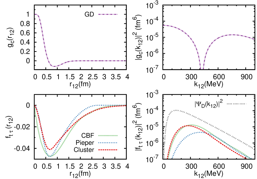
Figure 1: (color online). The radial and momentum dependence of a central and some tensor correlation functions. The central correlation function “GD” is for nuclear matter and from Ref. Gearheart (1994). The tensor correlation function “Pieper” is for ¹⁶O and from Ref. Pieper et al. (1992), the “CBF” one is for ¹⁶O and from Ref. Arias de Saavedra et al. (1996), and the “cluster” one is for ¹⁶O and from Ref. Alvioli et al. (2005), $\Psi_{D}\left(k_{12}\right)$ is the $l=2$ component of the non-relativistic deuteron wave function generated with the Paris potential Lacombe et al. (1980, 1981) (not to scale).

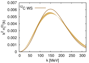
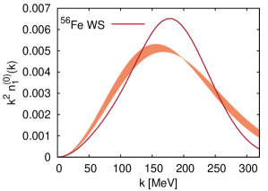
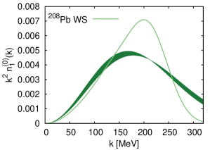
Figure 2: (color online). The computed $k^{2}n^{(0)}_{1}(k)$ versus $k$ for the nuclei ¹²C, ⁵⁶Fe and ²⁰⁸Pb and a Boltzmann fit including the error bars. The extracted values of $kT$ are 12.0$\pm 0.5$ MeV (C), 14$\pm 1$ MeV (Fe), and 16$\pm 1$ MeV (Pb). The calculations are performed with WS single-particle states. The adopted normalization convention is $\int dk\;k^{2}\;n^{(0)}_{1}(k)=1$.

After introducing the wave functions of Eq. (15), the one-body and two-body momentum distributions of Eqs. (1) and (7) can be written as

$$P_{1}\left(\vec{k}\right) = P^{(0)}_{1}\left(\vec{k}\right)+P^{(1)}_{1}\left(\vec{k}\right)\;,$$ (18)

$$P_{2}\left(\vec{k}_{12},\vec{P}_{12}\right) = P^{(0)}_{2}\left(\vec{k}_{12},\vec{P}_{12}\right)+P^{(1)}_{2}\left(\vec{k}_{12},\vec{P}_{12}\right)\;.$$

The $P^{(0)}_{1}$ and $P^{(0)}_{2}$ are the mean-field parts and are fully determined by the Slater determinant $\mid\Psi_{A}^{MF}\ \rangle$. After inserting the expressions (1) and (2) into the Eq. (13) one obtains

$$n^{(0)}_{1}\left({k}\right) = \int d\Omega_{k}P^{(0)}_{1}\left(\vec{k}\right)=\frac{2}{\pi}\sum_{n_{h}l_{h}j_{h}}\left(2j_{h}+1\right)S_{n_{h}l_{h}j_{h}}$$ (20)

$$\times\left(\int drr^{2}j_{l_{h}}(kr)\psi_{n_{h}l_{h}j_{h}}(r)\right)^{2}\;,$$

where $j_{l}(r)$ is the spherical Bessel function of the first kind and the sum extends over all occupied single-particle states. The $0\leq S_{n_{h}l_{h}j_{h}}\leq 1$ is the occupation probability of the corresponding single-particle state. The presence of short-range and long-range correlations leads to occupation probabilities smaller than one. With the adopted normalization convention of Eq. (4) one typically obtains that

$$\int dkk^{2}n^{(0)}_{1}\left({k}\right)\approx 0.6-0.8\;,$$ (21)

or, about $60-80\%$ of the nucleons are mean-field like. We stress that a considerable fraction of this depletion can be attributed to long-range correlations, an effect which is not considered here.

The distribution $k^{2}n^{(0)}_{1}(k)$ as it can be computed from Eq. (20) is reminiscent for a phenomenon which is confined to a certain scale, or, in other words, it is Gaussian like. The typical scale is determined by the Fermi momentum $k_{F}\approx 250~{}\textrm{MeV}$. This is illustrated in Fig. 2 where we show the momentum dependence of the $k^{2}n^{(0)}_{1}(k)$ for ¹²C, ⁵⁶Fe and ²⁰⁸Pb as computed with Woods-Saxon (WS) wave functions. For the sake of curiosity we have fitted the computed $k^{2}n^{(0)}_{1}(k)$ with a Boltzmann distribution

$$\frac{4\pi}{\left(2\pi M_{N}kT\right)^{3/2}}k^{2}\exp-\frac{k^{2}}{2M_{N}kT}\;.$$ (22)

The results of the one-parameter fit are shown in Fig. 2. The fit is remarkably good for Carbon and gets increasingly inaccurate with increasing mass number. From the fit of the Boltzmann distribution we obtain $kT\approx 12$ MeV (C), $kT\approx 14$ MeV (Fe), $kT\approx 16$ MeV (Pb). Accordingly, for the IPM part of the momentum distribution, the typical energy exchange per momentum degree-of-freedom $\frac{1}{2}kT$ is of the order of 6-8 MeV.

The correlated part $k^{2}n^{(1)}_{1}(k)$, on the other hand, is reminiscent of the nucleus as a system of interdependent nucleons and is obviously non-Gaussian. In contrast to the mean-field part $n^{(0)}_{1}$, the correlated part $n^{(1)}_{1}$ extends over “all” momentum scales. Or, in other words the 2N, 3N, $\ldots$ correlations generate a fat momentum tail to the $n_{1}\left(k\right)$. The high momentum tails to $n_{1}\left(k\right)$ have a very similar form for all nuclei, including the deuteron, which alludes to some universal character of SRC Feldmeier et al. (2011).

It has been theoretically predicted Frankfurt and Strikman (1988); Ciofi degli Atti and Simula (1996); Janssen et al. (2000) and experimentally confirmed in semi-exclusive $A(e,e^{\prime}p)$ measurements Iodice et al. (2007) that the major fraction of the $n_{1}^{(1)}\left(k>k_{F}\right)$ strength is contained in very specific parts of the single-nucleon removal energy-momentum phase space, namely those where the ejected nucleon is part of a pair with high relative and small c.m. momentum. This is the so-called ridge in the spectral function Janssen et al. (2000) which reflects the fact that high-momentum nucleons in the one-body momentum distribution are related to 2N dynamics with two nucleons which are close and move back-to-back with approximately equal and opposite momenta.

From recent calculations Alvioli et al. (2012) of the two-body momentum distributions in ³He and ⁴He the following conclusions could be drawn. At high relative momenta and small c.m. momenta, the c.m. and relative motion of the pair is decoupled, an effect which is reminiscent of 2N SRC. For the correlated pn pairs the relative motion can be described by the high-momentum part of the deuteron wave function. This suggests the following expression for the correlated part of the pn two-body momentum distribution

$$n^{(1)}_{2} \left(2k_{F}\lesssim k_{12},P_{12}\lesssim 150~{}\textrm{MeV}\right)$$ (23)

$$\approx a_{pn}\left(A,Z\right){n}_{D}\left(k_{12}\right)F^{pn}\left(P_{12}\right)\;,$$

where $a_{pn}\left(A,Z\right)$ is a proportionality factor related to the number of correlated proton-neutron pairs in the nucleus ${}^{A}Z$ relative to the deuteron and ${n}_{D}\left(k_{12}\right)$ is the high-$k_{12}$ deuterium momentum distribution. Further, the $F^{pn}\left(P_{12}\right)$ is the c.m. distribution of the correlated pn pairs. It corresponds with that part of $P_{2}\left(P_{12}\right)$ of Eq. (11) that stems from pn pairs with a zero relative orbital angular momentum $l_{12}=0$ and a total spin $S=1$. The proposed scaling behavior (23) can be attributed to the dominance of the tensor correlations at medium relative momenta and the fact that $\mid f_{t\tau}\left(k_{12}>k_{F}\right)\mid^{2}\sim\left|\Psi_{D}\left(k_{12}\right)\right|^{2}$, two qualitative observations which can made from Fig. 1.

II.3 Quantifying two-nucleon correlations

We suggest that the significance of 2N correlations in a nucleus $A(N,Z)$ is proportional to the number of relative $l_{12}=0$ states Vanhalst et al. (2011). There are experimental results supporting this conjecture. First, in high-resolution ¹⁶O$(e,e^{\prime}pp)^{14}$N measurements performed at the electron accelerators in Amsterdam Starink et al. (2000) and Mainz Ryckebusch and Van Nespen (2004), the quantum numbers of the target nucleus and the residual nucleus are unambiguously determined. For the transitions to low-lying states in the residual nucleus, the eightfold differential cross section for the exclusive $(e,e^{\prime}pp)$ reaction has been studied as a function of the initial c.m. momentum $P_{12}$ of the proton-proton pair which is involved in the reaction process. This has provided insight into the quantum numbers of the pairs involved in the reaction process. We denote by $\left|l_{12}\left(\vec{r}_{12}\right),\Lambda_{12}\left(\vec{R}_{12}\right)\right>$ the orbital wave function corresponding with the relative and c.m. motion of a nucleon pair. For the ground-state (g.s.) to g.s. transition, for example,

$${}^{16}\textrm{O}(0^{+},g.s.)+e\longrightarrow^{14}\textrm{C}(0^{+},g.s.)+e^{\prime}+pp\;,$$ (24)

the active diproton resides in a state with quantum numbers $\left|l_{12}=0,\Lambda_{12}=0\right>$ at lower $P_{12}$ and $\left|l_{12}=1,\Lambda_{12}=1\right>$ at higher $P_{12}$. Two independent calculations from the Pavia and Ghent groups have demonstrated that the largest contributions from SRC to the eight-fold cross section are confined to low $P_{12}$ values Ryckebusch and Van Nespen (2004). This provides direct evidence of pp correlations being confined to $\left|l_{12}=0,\Lambda_{12}=0\right>$ pairs. In that sense, the ¹⁶O$(e,e^{\prime}pp)^{14}$N measurements nicely confirmed the back-to-back picture of SRC: diprotons are subject to SRC whenever they happen to be close (or, in a relative $l_{12}=0$ state) and moving back-back (or, in a state with $P_{12}\approx 0$ which corresponds with $\Lambda_{12}=0$).

High-resolution $(e,e^{\prime}pn)$ measurements which have the potential to access the pn correlations are very challenging Middleton et al. (2007). Theoretical $(e,e^{\prime}pn)$ calculations Janssen et al. (2000); Ryckebusch et al. (2000); Barbieri et al. (2004) have predicted that the tensor parts of the SRC are responsible for the fact that the correlated pn strength is typically a factor of 10 bigger than the correlated pp strength. Calculations indicated that the tensor correlations are strongest for pn pairs pairs with “deuteron-like” $\left|l_{12}=0,S=1\right>$ relative states Ryckebusch et al. (2000); Barbieri et al. (2004). Recently, the dominance of the pn correlations over pp and nn ones has been experimentally confirmed Subedi et al. (2008); Baghdasaryan et al. (2010).

Accordingly, a reasonable estimate of the amount of correlated nucleon pairs in $A(N,Z)$ is provided by the number of pairs in a $l_{12}=0$ state. In order to determine that number for a given set of single-particle states, one needs a coordinate transformation from $(\vec{r}_{1},\vec{r}_{2})$ to $\left(\vec{r}_{12}=\frac{\vec{r}_{1}-\vec{r}_{2}}{\sqrt{2}},\vec{R}_{12}=\frac{\vec{r}_{1}+\vec{r}_{2}}{\sqrt{2}}\right)$. For a harmonic oscillator (HO) Hamiltonian this transformation can be done with the aid of Moshinsky brackets Moshinsky and Smirnov (1996)

$$\mid n_{1}l_{1}\left(\vec{r}_{1}\right)n_{2}l_{2}\left(\vec{r}_{2}\right);LM_{L}\rangle=\sum_{n_{12}l_{12}N_{12}\Lambda_{12}}$$

$$\langle n_{12}l_{12}N_{12}\Lambda_{12};L\mid n_{1}l_{1}n_{2}l_{2};L\rangle$$

$$\times\mid n_{12}l_{12}\left(\vec{r}_{12}\right)N_{12}\Lambda_{12}\left(\vec{R}_{12}\right);LM_{L}\rangle\;.$$ (25)

We define the interchange operator for the spatial, spin, and isospin coordinate as

$$\mathcal{P}_{12}=\mathcal{P}_{12}\left(\vec{r}_{1},\vec{r}_{2}\right)\mathcal{P}_{12}\left(\vec{\sigma}_{1},\vec{\sigma}_{2}\right)\mathcal{P}_{12}\left(\vec{\tau}_{1},\vec{\tau}_{2}\right)\;.$$ (26)

After introducing the spin and isospin degrees-of-freedom, in a HO basis a normalized and antisymmetrized two-nucleon state reads ($\alpha_{i}\equiv(n_{i}l_{i}j_{i}t_{i})$)

$$\left|\alpha_{1}\alpha_{2};JM\right>_{na}=\frac{1}{\sqrt{2\left(1+\delta_{\alpha_{1}\alpha_{2}}\right)}}$$

$$\times\left(1-\mathcal{P}_{12}\right)\left|\alpha_{1}\left(\vec{r}_{1}\right)\alpha_{2}\left(\vec{r}_{2}\right);JM\right>$$

$$=\sum_{LM_{L}}\sum_{n_{12}l_{12}}\sum_{N_{12}\Lambda_{12}}\sum_{SM_{S}}\sum_{TM_{T}}\frac{1}{\sqrt{2\left(1+\delta_{\alpha_{1}\alpha_{2}}\right)}}$$

$$\times\left[1-(-1)^{l_{12}+S+T}\right]$$

$$\times\langle n_{12}l_{12}N_{12}\Lambda_{12};L\mid n_{1}l_{1}n_{2}l_{2};L\rangle$$

$$\times\hat{j_{1}}\hat{j_{2}}\hat{L}\hat{S}\begin{Bmatrix}l_{1}&l_{2}&L\\ \frac{1}{2}&\frac{1}{2}&S\\ j_{1}&j_{2}&J\end{Bmatrix}\langle LM_{L}SM_{S}\mid JM\rangle\;$$

$$\times\langle\frac{1}{2}t_{1}\frac{1}{2}t_{2}\mid TM_{T}\rangle$$

$$\times\left|\left[{n_{12}l_{12}\left(\vec{r}_{12}\right)},{N_{12}\Lambda_{12}\left(\vec{R}_{12}\right)}\right]LM_{L},SM_{S},TM_{T}\right>\;,$$

(27)

where we have used the shorthand notation $\hat{j}\equiv\sqrt{2j+1}$.

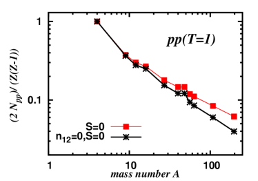
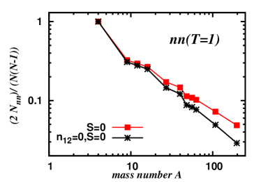
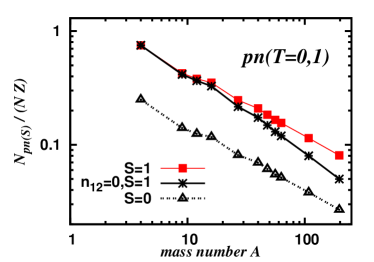
Figure 3: (color online). The computed values for $\frac{2}{Z(Z-1)}N_{pp}$, $\frac{2}{N(N-1)}N_{nn}$, and $\frac{1}{(NZ)}N_{pn(S)}$ which represent the predicted fraction of the pairs which are prone to SRC. The results are obtained for HO single-particle wave functions with $\hbar\omega(MeV)=45.A^{-\frac{1}{3}}-25.A^{-\frac{2}{3}}$ and for the target nuclei ⁴He, ⁹Be, ¹²C, ¹⁶O, ²⁷Al, ⁴⁰Ca, ⁴⁸Ca, ⁵⁶Fe, ⁶³Cu, ¹⁰⁸Ag, and ¹⁹⁷Au.

With the above conventions one has that the total amount of proton-neutron pairs can be obtained from a sum over all pn pairs in the nuclear ground state

$$\sum_{JM}\sum_{\alpha_{1}\leq\alpha_{F}^{p}}\sum_{\alpha_{2}\leq\alpha_{F}^{n}}\;{}_{na}\left<\alpha_{1}\alpha_{2};JM\right.\left|\alpha_{1}\alpha_{2};JM\right>_{na}=NZ\;,$$ (28)

where $\alpha_{F}^{p}$ and $\alpha_{F}^{n}$ denote the Fermi level for the proton and neutron. Similar expressions hold for the number of proton-proton and neutron-neutron pairs

$$\frac{Z(Z-1)}{2}=\sum_{JM}\sum_{\alpha_{1}\leq\alpha_{F}^{p}}\sum_{\alpha_{2}\leq\alpha_{F}^{p}}$$

$$\;{}_{na}\left<\alpha_{1}\alpha_{2};JM\right.\left|\alpha_{1}\alpha_{2};JM\right>_{na}\;,$$ (29)

$$\frac{N(N-1)}{2}=\sum_{JM}\sum_{\alpha_{1}\leq\alpha_{F}^{n}}\sum_{\alpha_{2}\leq\alpha_{F}^{n}}$$

$$\;{}_{na}\left<\alpha_{2}\alpha_{2};JM\right.\left|\alpha_{1}\alpha_{2};JM\right>_{na}\;.$$ (30)

Starting from the Eq. (27) one can compute in a HO single-particle basis how much a pair wave function with quantum numbers

$$\left|\left[n_{12}l_{12}\left(\vec{r}_{12}\right),N_{12}\Lambda_{12}\left(\vec{R}_{12}\right)\right]LM_{L},SM_{S},TM_{T}\right>$$ (31)

contributes to the sum-rules of Eqs. (28,29,30). This can also be done for any other basis $\left|nljm\right>$ of non-relativistic single-particle states. In that case, the adopted procedure involves an extra expansion of $\left|nljm\right>$ in a HO basis

$$\left|nljm\right>=\sum_{m_{l}m_{s}}\langle lm_{l}\frac{1}{2}m_{s}\mid jm\rangle\psi_{nlj}(r)Y_{lm_{l}}\left(\Omega\right)\chi_{\frac{1}{2}m_{s}}$$ (32)

$$= \sum_{n_{H}}\left(\int drr^{2}\phi_{n_{H}l}^{*}(r)\psi_{nlj}(r)\right)\left|n_{H}ljm\right>\;,$$

where $\phi_{n_{H}l}(r)$ are the radial HO wave functions. A two-nucleon state can then be expressed in a HO basis for which the Eq. (27) can be used to determine the weight of the pair wave functions of Eq. (31).

The IPM pp pairs are mainly subject to the central SRC which requires them to be close. This implies that a reasonable estimate of the number of IPM pp pairs which receive substantial corrections from the SRC is given by an expression of the type

$$N_{pp}(A,Z)=\sum_{JM}\sum_{\alpha_{1}\leq\alpha_{F}^{p}}\sum_{\alpha_{2}\leq\alpha_{F}^{p}}$$

$${}_{na}\left<\alpha_{1}\alpha_{2};JM\right|\mathcal{P}_{\vec{r}_{12}}^{l_{12}=0}\left|\alpha_{1}\alpha_{2};JM\right>_{na}\;,$$ (33)

where $\mathcal{P}_{\vec{r}_{12}}^{l_{12}=0}$ is a projection operator for two-nucleon relative states with $l_{12}=0$. A similar expression to Eq. (33) holds for the nn pairs. For the pn pairs it is important to discriminate between the triplet and singlet spin states

$$N_{pn(S)}(A,Z)=\sum_{JM}\sum_{\alpha_{1}\leq\alpha_{F}^{p}}\sum_{\alpha_{2}\leq\alpha_{F}^{n}}$$

$${}_{na}\left<\alpha_{1}\alpha_{2};JM\right|\mathcal{P}_{\vec{r}_{12}}^{l_{12}=0}\mathcal{P}_{\vec{\sigma}}^{S}\left|\alpha_{1}\alpha_{2};JM\right>_{na}\;.$$ (34)

In Fig. 3 we display some computed results for the $N_{pp}$, $N_{nn}$, and $N_{pn(S)}$ for 11 nuclei. The selection of the nuclei is motivated by the availability of inclusive electron-scattering data and covers the full mass range from Helium to Gold. We have opted to display the results relative to the sum rule values of the Eqs. (28) and (29), which allows one to interpret the results in terms of probabilities: given an arbitrary pair wave function, what is the chance that it has zero orbital relative momentum and a specific spin quantum number. In a naive IPM picture for ⁴He, the pp pair is in a $\left|l_{12}=0,S=0,T=1\right>$ state. As this 2N configuration is prone to central SRC effects, the corresponding probability is 1. The physical interpretation is that for ⁴He “all” IPM pp-pair wave function combinations receive corrections from SRC. For a medium-heavy nucleus like ⁵⁶Fe or ⁶³Cu we find $\frac{N_{pp}}{\frac{Z(Z-1)}{2}}\approx 0.1$, which leads one to conclude that about 90% of the IPM pp pair wave functions do not receive corrections from central SRC. For the heaviest nucleus considered here (Au) $\frac{2N_{pp}}{Z(Z-1)}=0.06$, which means that only about 190 out of the 3081 possible pp pair combinations are subject to SRC.

Comparing the mass dependence of the pp and nn results of Fig. 3 one observes similar trends. For the pn results a softer decrease with increasing $A$ is predicted. There are about three times as many pn$(T=0)$ states than pn$(T=1)$ states with $l_{12}=0$. This would be trivial in a system with only spin and isospin degrees of freedom. In a system in which the kinetic energy plays a role and in which there are spin-orbit couplings, we cannot see any trivial reason why this should be the case. In this respect, we wish to stress that for most nuclei discussed $N\neq Z$. A stronger criterion for selecting nucleon pairs at close proximity is imposing $n_{12}=0$ in addition to $l_{12}=0$ and we have added also those results to Fig. 3. We find the results of Fig. 3 robust in that the A dependence and magnitudes are not very sensitive to the choices made with regard to the single-particle wave functions. All the results of Fig. 3 are displayed on a log-log plot and can be reasonably fitted with a straight line, pointing towards a power-law mass dependence $A^{\alpha}$ for the $N_{pp}$, $N_{pn}$ and $N_{pn(S)}$.

II.4 Quantifying three-nucleon correlations

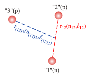
Figure 4: (color online). Use of Jacobi coordinates in the ppn system.

In order to quantify the magnitude of the 3N correlations for an arbitrary $A(N,Z)$, we build on a recent paper by Feldmeier et al. Feldmeier et al. (2011). There, it is pointed out that 3N correlations can be induced without introducing genuine three-body forces. In terms of the correlation operators of Sect. II.2, three-body correlations will naturally emerge in cluster expansions by means of operators of the type $g_{c}\left(r_{12}\right)g_{c}\left(r_{13}\right)$, $g_{c}\left(r_{12}\right)f_{t\tau}\left(r_{13}\right)$, $\ldots\;$.

The strongest source of three-nucleon correlations is the tensor correlation operator acting on the $(S=1,T=0)$ channel of the pn states of Eq. (27). We consider ppn configurations and explain one possible mechanism to create a correlated state (see also Fig. 4). In the uncorrelated wave function one has a n(1)p(2) pair in a $\left|l_{12}=0\;\;S_{12}=1\;;T_{12}=0\right>$ state and a p(2)p(3) pair in a $\left|l_{23}=0\;\;S_{23}=0\;;T_{23}=1\right>$ state. Accordingly, both pairs are in relative $l=0$ states. In Ref. Feldmeier et al. (2011) it is explained that these two pairs can be brought into a correlated three-nucleon status by flipping the spin of proton 2. In the correlated part of the wave function one has an n(1)p(2) pair in a $\left|l_{12}=2\;\;S_{12}=1\;;T_{12}=0\right>$ and an p(2)p(3) pair in a $\left|l_{23}=1\;\;S_{23}=1\;;T_{23}=1\right>\;$ state. This configuration can be energetically favorable through the presence of the strong tensor correlation in the pn pair. Indeed, the energy gain through the tensor induced n(1)p(2) correlation can compensate for the energy loss of breaking the pairing in the p(2)p(3) pair.

Given $A(N,Z)$ we propose to find all the antisymmetrized 3N states with orbital quantum numbers

$$(n_{12}=0\;l_{12}=0\;n_{(12)3}=0\;l_{(12)3}=0)\;,$$ (35)

in the IPM wave function and identify them as the dominant contributors to 3N SRCs. This corresponds with seeking for those 3N wave-function components where all three nucleons are “close”. This can be technically achieved by constructing antisymmetrized 3N states starting from a MF Slater determinant, and performing a transformation from the particle coordinates $\left(\vec{r}_{1},\vec{r}_{2},\vec{r}_{3}\right)$ to the internal Jacobi coordinates $\left(\vec{r}_{12},\vec{r}_{(12)3},\vec{R}_{123}\right)$

$$\vec{r}_{(12)3}=\frac{\vec{R}_{12}-\sqrt{2}\vec{r}_{3}}{\sqrt{3}},\hskip 21.68231pt\vec{R}_{123}=\frac{\sqrt{2}\vec{R}_{12}+\vec{r}_{3}}{\sqrt{3}}\;.$$ (36)

One readily finds for uncoupled three-nucleon states in a HO basis Moshinsky and Smirnov (1996)

$$\left|n_{1}l_{1}m_{l_{1}}\left(\vec{r}_{1}\right),n_{2}l_{2}m_{l_{2}}\left(\vec{r}_{2}\right),n_{3}l_{3}m_{l_{3}}\left(\vec{r}_{3}\right)\right>=$$

$$\sum_{LM_{L}}\sum_{n_{12}l_{12}}\sum_{N_{12}\Lambda_{12}}\sum_{L_{1}M_{L_{1}}}\sum_{n_{(12)3}l_{(12)3}}$$

$$\times\sum_{N_{123}\Lambda_{123}}\sum_{m_{l_{12}}m_{\Lambda_{12}}}\sum_{m_{l_{(12)3}}m_{\Lambda_{123}}}$$

$$\times\langle l_{1}m_{l_{1}}l_{2}m_{l_{2}}\mid LM_{L}\rangle\langle l_{12}m_{l_{12}}\Lambda_{12}M_{\Lambda_{12}}\mid LM_{L}\rangle$$

$$\times\langle\Lambda_{12}M_{\Lambda_{12}}l_{c}m_{l_{c}}\mid L_{1}M_{L_{1}}\rangle$$

$$\times\langle l_{(12)3}m_{l_{(12)3}}\Lambda_{123}M_{\Lambda_{123}}\mid L_{1}M_{L_{1}}\rangle$$

$$\times\langle n_{12}l_{12}N_{12}\Lambda_{12};L\mid n_{1}l_{1}n_{2}l_{2};L\rangle$$

$$\times\langle n_{(12)3}l_{(12)3}N_{123}\Lambda_{123};L_{1}\mid N_{12}\Lambda_{12}n_{3}l_{3};L_{1}\rangle_{\beta}$$

$$\times\left|n_{12}l_{12}m_{l_{12}}\left(\vec{r}_{12}\right)\right>\left|n_{(12)3}l_{(12)3}m_{l_{(12)3}}\left(\vec{r}_{(12)3}\right)\right>$$

$$\times\left|N_{123}\Lambda_{123}M_{\Lambda_{123}}\left(\vec{R}_{123}\right)\right>\;,$$ (37)

where we have adopted the notation $\langle\ldots\mid\ldots\rangle_{\beta}$ for the Standard Transformation Brackets (STB) Moshinsky and Smirnov (1996).

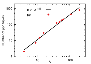
Figure 5: (color online). The mass dependence of the amount of ppn triples with quantum numbers $\left|n_{12}=0\;l_{12}=0,n_{(12)3}=0\;l_{(12)3}=0\right>$. The results can be reasonably fitted with a power law $0.28A^{1.58\pm 0.20}$. The results are obtained for HO single-particle wave functions with $\hbar\omega(MeV)=45.A^{-\frac{1}{3}}-25.A^{-\frac{2}{3}}$ and for the nuclei ⁴He, ⁹Be, ¹²C, ¹⁶O, ⁴⁰Ca, ⁴⁸Ca, ⁵⁶Fe, ⁶³Cu, ¹⁰⁸Ag, and ¹⁹⁷Au.

Antisymmetrized $(a)$ uncoupled three-nucleon states can be obtained from the three-nucleon wave functions of Eq. (37) using the interchange operator of Eq. (26)

$$\left|\alpha_{a}m_{a},\alpha_{b}m_{b},\alpha_{c}m_{c}\right>_{a}=$$ (38)

$$\left[1-\mathcal{P}_{12}\right]\left|\alpha_{a}m_{a}\left(\vec{r}_{1}\right),\alpha_{b}m_{b}\left(\vec{r}_{2}\right),\alpha_{c}m_{c}\left(\vec{r}_{3}\right)\right>$$

$$+ \left[1-\mathcal{P}_{12}\right]\left|\alpha_{b}m_{b}\left(\vec{r}_{1}\right),\alpha_{c}m_{c}\left(\vec{r}_{2}\right),\alpha_{a}m_{a}\left(\vec{r}_{3}\right)\right>$$

$$+ \left[1-\mathcal{P}_{12}\right]\left|\alpha_{c}m_{c}\left(\vec{r}_{1}\right),\alpha_{a}m_{a}\left(\vec{r}_{2}\right),\alpha_{b}m_{b}\left(\vec{r}_{3}\right)\right>\;.$$

The total number of ppn triples can now be expressed as

$$N\frac{Z(Z-1)}{2}=\sum_{\alpha_{a},\alpha_{b}\leq\alpha_{F}^{p}}\sum_{\alpha_{c}\leq\alpha_{F}^{n}}\sum_{m_{a}m_{b}m_{c}}$$

$$\;{}_{na}\left<\alpha_{a}m_{a},\alpha_{b}m_{b},\alpha_{c}m_{c}\right.\left|\alpha_{a}m_{a}\alpha_{b}m_{b}\alpha_{c}m_{c}\right>_{na}\;,$$ (39)

which allows for a stringent test of the analytical derivations and their numerical implementation. Along similar lines to those used to derive the number of correlated 2N clusters in Eq. (33), the number of ppn triples with the orbital quantum numbers of Eq. (35) can be obtained from

$$N_{ppn}(A,Z)=\sum_{\alpha_{a},\alpha_{b}\leq\alpha_{F}^{p}}\sum_{\alpha_{c}\leq\alpha_{F}^{n}}\sum_{m_{a}m_{b}m_{c}}$$

$$\;{}_{na}\left<\alpha_{a}m_{a},\alpha_{b}m_{b},\alpha_{c}m_{c}\right|\mathcal{P}_{\vec{r}_{12}}^{n_{12}=0,l_{12}=0}\mathcal{P}_{\vec{r}_{(12)3}}^{n_{(12)3}=0,l_{(12)3}=0}$$

$$\left|\alpha_{a}m_{a},\alpha_{b}m_{b},\alpha_{c}m_{c}\right>_{na}\;.$$ (40)

We associate the $N_{ppn}(A,Z)$ with the number of ppn SRC triples. The $A$ dependence of $N_{ppn}(A,Z)$ is displayed in Fig. 5. There is striking linear correlation between the logarithm of the mass number and the logarithm of the number ppn triples which are close in the MF ground-state wave function.

III Results

In this section we discuss how our predictions for the number of correlated 2N pairs and correlated 3N triples can be connected with experimental results from inclusive electron scattering.

III.1 Separation of the correlation and mean-field contributions

We start with illustrating that the separation of the mean-field and correlated contributions to the inclusive $A(e,e^{\prime})$ cross sections is feasible. In order to achieve this, we use stylized features of the $n_{1}(k)$ in Monte-Carlo (MC) simulations to illustrate that a separation between the mean-field $n_{1}^{(0)}(k)$ and the correlated $n_{1}^{(1)}(k)$ part can be made in the $A(e,e^{\prime})$ signal.

We assume that quasi-elastic single-nucleon knockout $e+A\rightarrow e^{\prime}+(A-1)+N$ is the major source of $A(e,e^{\prime})$ strength. With $q(\omega,\vec{q})$, $p_{A}(M_{A},\vec{0})$, $p_{A-1}(E_{A-1},\vec{p}_{A-1})$, $p_{f}(E_{N},\vec{p}_{f})$ we denote the four-momenta of the virtual photon, of the target nucleus, of the residual $A-1$ system, and of the ejected nucleon. From energy-momentum conservation

$$q+p_{A}-p_{A-1}=p_{f},$$ (41)

one can deduce for $A=2$ a relation between the minimum of the missing momentum $\vec{p}_{m}=\vec{p}_{f}-\vec{q}$ and the Bjorken scaling variable $x_{B}$ for fixed $Q^{2}$ Sargsian (2001). The results are shown in Fig. 6. Obviously, for $Q^{2}\geq 1.5$ GeV² and $x_{B}>1.5$ one mainly probes nucleons with a momentum well above the Fermi momentum for the deuteron. For finite nuclei the situation is more involving as $A-1$ represents an additional degree of freedom which can carry a fraction of the transferred four-momentum. We have performed MC simulations for a fixed energy of the impinging electron beam $\epsilon_{i}$ and a fixed electron scattering angle $\theta_{e}$. The $p_{m}$ for a mean-field nucleon is drawn from the MF part $n_{1}^{(0)}(k)$ of $n_{1}(k)$. For a correlated nucleon the $p_{m}$ is drawn from $n_{1}^{(1)}(k)$. Parameterizations for $n_{1}^{(0)}(k)$ and $n_{1}^{(1)}(k)$ are obtained from Ciofi degli Atti and Simula (1996)

$$n_{1}^{(0)}(k) = A^{(0)}e^{-B^{(0)}k^{2}}[1+\mathcal{O}(k^{2})],$$ (42)

$$n^{(1)}_{1}(k) = A^{(1)}e^{-B^{(1)}k^{2}}+C^{(1)}e^{-D^{(1)}k^{2}},$$ (43)

where $A^{(0)}$, $B^{(0)}$, $A^{(1)}$, $B^{(1)}$, $C^{(1)}$ and $D^{(1)}$ depend on $A$.

In Fig. 7 we compare the $x_{B}$ distribution of simulations for the mean-field and correlated part of one nucleon knockout in ¹²C. As stated in Eq. (21), the number of events is normalized as $\int\mathrm{d}k\;k^{2}n_{1}^{(0)}(k)=0.7$. For $x_{B}>1.5$, the events originate almost uniquely from $n^{(1)}_{1}(k)$.

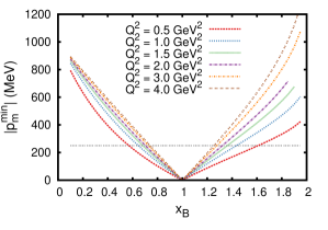
Figure 6: (Color online). Relation between the minimum of the missing momentum $|p_{m}^{min}|$ for the deuteron and $x_{B}$ at various values of the frour-momentum transfer $Q^{2}$.

Figure 7: (Color online). Simulation of one-nucleon knockout in ¹²C with separated mean field and correlated momentum distribution. The number of events is normalized as in Eq. (21). The electron kinematics is determined by $\epsilon_{i}=$5.766\text{\,}\mathrm{GeV}$$ and $\theta_{e}=$18\text{\,}\mathrm{\SIUnitSymbolDegree}$$.

III.2 Two-body correlations

Following the experimental observation Frankfurt et al. (1993); Egiyan et al. (2006); Fomin et al. (2012) that the ratio of the inclusive electron scattering cross sections from a target nucleus $A$ and from the deuteron $D$

$$\frac{\sigma^{A}\left(x_{B},Q^{2}\right)}{\sigma^{D}\left(x_{B},Q^{2}\right)}\;,$$ (44)

scales for $1.5\lesssim x_{B}\lesssim 2$ and moderate $Q^{2}$, it has been suggested Frankfurt et al. (1993) to parameterize the $\sigma^{A}$ in the following form

$$\sigma^{A}\left(1.5\lesssim x_{B}\lesssim 2,Q^{2}\right)=\frac{A}{2}a_{2}\left({A}/{D}\right)\sigma_{2}\left(A,x_{B},Q^{2}\right)\;,$$ (45)

where $\sigma_{2}\left(A,x_{B},Q^{2}\right)$ is the effective cross section for scattering from a correlated 2N cluster in nucleus $A$. Assuming that $\sigma_{2}$ is some local function which does not depend on the target nucleus $A$

$$\sigma_{2}\left(A,x_{B},Q^{2}\right)\approx\sigma_{2}\left(A=2,x_{B},Q^{2}\right)\approx\sigma^{D}\left(x_{B},Q^{2}\right),$$ (46)

one can rewrite Eq. (45) as

$$a_{2}\left({A}/{D}\right)=\frac{2}{A}\frac{\sigma^{A}\left(x_{B},Q^{2}\right)}{\sigma^{D}\left(x_{B},Q^{2}\right)}\;\;\left(1.5\lesssim x_{B}\lesssim 2\right)\;.$$ (47)

In this simplified reaction-model picture, which ignores amongst other things the c.m. motion of pairs in finite nuclei, the quantity $\frac{A}{2}a_{2}\left({A}/{D}\right)$ can be connected with the number of correlated pairs in the nucleus $A$. Assuming that all pn pairs contribute one would expect that for the relative amount of correlated two-nucleon clusters $a_{2}\left({A}/{D}\right)\sim A$. Based on the observed dominance of correlated pn pairs over pp and nn pairs Subedi et al. (2008), and the universality of the deuteron-like high momentum tail of the correlated two-body momentum distribution (23), we suggest that the correlated pn pairs contributing to the $a_{2}(A/D)$, are predominantly $(T=0,S=1)$ pairs and that $a_{2}(A/D)$ is proportional to the quantity $N_{pn(S=1)}(A,Z)$ defined in Eq. (34).

In Ref. Benhar et al. (1995) the ratio of Eq.  (44) has been calculated with spectral functions obtained from state-of-the-art nuclear matter calculations in the local density approximation for the correlated part and $A(e,e^{\prime}p)$ scattering data for the mean-field part Benhar et al. (1994); Sick et al. (1994). The calculations suggested large FSI effects, whilst the plane-wave calculations did not exhibit the scaling present in the data at $1.5\lesssim x_{B}$. In Refs. Arrington et al. (2012b); Frankfurt et al. (2008) it is argued that a complete treatment of FSI in this kinematics needs to include inelastic channels in the rescattering and that this cancels part of the elastic FSI contribution included in Ref. Benhar et al. (1995). The results in Ref. Benhar et al. (1995) seem to refute the validity of Eq. (45), which hinges on the assumption that the FSI effects on correlated pairs in a nucleus are almost identical to those in the deuteron in a high-momentum state. This requires that for $1.5\lesssim x_{B}$ the FSI is primarily in the correlated pair and that the remaining $A-2$ nucleons act as spectators. Such a behavior is suggested by the calculation of the quasi-elastic cross sections in Ref. Ciofi degli Atti and Simula (1994) and by a space-time analysis of the nuclear FSI at $x_{B}>1$ carried out in Ref. Frankfurt et al. (2008) where it is stressed that the reinteraction distances are $\lesssim 1~{}$fm, supporting the idea that the first rescattering should be very similar to FSI in the deuteron (see a recent discussion in Ref. Arrington et al. (2012b)). Therefore the assumption of Eq. (45) seems a reasonable one for light nuclei where the amount of rescatterings is of the order of 1. For medium-heavy and heavy nuclei, the average amount of rescatterings is larger than 1 and it has to be verified if the assumption still holds. The settlement and clarification of all the cited issues related to the role of FSI in inclusive reactions requires further studies with a full reaction model.

In a finite nucleus correlated pairs can have a non-zero c.m. momentum. This c.m. motion is a correction factor when connecting the measured $a_{2}(A/D)$ to the number of correlated pn pairs $N_{pn(S=1)}(A,Z)$. We aim to provide an estimate for this correction factor. Therefore, we consider the two-nucleon knockout reaction $e+A\rightarrow e^{\prime}+(A-2)+N+N$ following the break-up of a correlated 2N cluster. For an inclusive cross section, the tensor correlated pn$(S=1)$ pairs dominate the signal Piasetzky et al. (2006); Subedi et al. (2008); Baghdasaryan et al. (2010).

As pointed out in Refs. Frankfurt et al. (2008); Ryckebusch (1996), the cross section for the exclusive $(e,e^{\prime}NN)$ reaction can be written in a factorized form as

$$\sigma^{A}(e,e^{\prime}NN)=KF^{NN}(P_{12})\sigma_{eNN}(k_{12})\,,$$ (48)

where $P_{12}(k_{12})$ is the c.m. (relative) momentum of the correlated pair on which the photoabsorption takes place and $K$ is a kinematic factor. The above expression is valid in the plane-wave and spectator approximation for electron scattering on a pair with zero relative orbital momentum. The $\sigma_{eNN}$ stands for the elementary cross section for electron scattering from a correlated 2N pair with relative momentum $k_{12}$. The $\sigma_{eNN}$ contains the Fourier-transformed correlation functions $g_{c}(k_{12})$ and $f_{t\tau}(k_{12})$. An analytic expression for $\sigma_{epp}$ is contained in Ref. Ryckebusch (1996) and has been tested against data in Ref. Blomqvist et al. (1998).

As argued above, in order to link the exclusive cross section of Eq. (48) to the inclusive ones contained in the Eq. (45) one assumes that $\sigma_{epn}\approx\sigma_{eD}$ and one introduces a proportionality factor $N_{pn(S=1)}(A,Z)$ which counts the number of correlated pn pairs in $A$. With the scaling relation of Eq. (48) for the $(e,e^{\prime}pn)$ reaction, one can transform the ratio of Eq. (47) into a form which accounts for the c.m. motion of the pair

$$a_{2}(A/D)=\frac{2}{A}$$ (49)

$$\times\frac{\int_{PS}\mathrm{d}\vec{k}_{12}\mathrm{d}\vec{P}_{12}N_{pn(S=1)}(A,Z)F^{pn}(P_{12})\sigma_{eD}\left(k_{12}\right)}{\int_{PS}d\vec{k}_{12}\sigma_{eD}(k_{12})}\;,$$

$$\approx \frac{2}{A}N_{pn(S=1)}(A,Z)\int_{PS}d\vec{P}_{12}F^{pn}\left(P_{12}\right)\;,$$

where the integrations extend over those part of the c.m. momentum phase (PS) included in the data. A basic assumption underlying the above equation is that the factorization of Eq. (23) approximately holds. The computed widths of the c.m. momentum distributions for the correlated pn pairs contained in Table 1 indicate that the major fraction of the pn pairs has $P_{12}\lesssim 150$ MeV which is within the ranges for the validity of Eq. (23).

In line with our assumption that the correlated pairs are dominated by pn in a relative ${}^{3}S_{1}$ state, $F^{pn}\left(P_{12}\right)$ can be expressed as the conditional two-body c.m. momentum distribution

$$F^{pn}\left(P_{12}\right)=P_{2}^{pn}\left(P_{12}|^{3}S_{1}\right).$$ (50)

Figure 8 shows calculations for the $P_{2}^{pn}\left(P\right)$ and $P_{2}^{pn}\left(P|^{3}S_{1}\right)$ for ¹²C. The c.m. distribution of correlated pn pairs ($F^{pn}(P_{12})$) can be well parameterized in terms of a Gaussian distribution. The widths $\sigma_{c.m.}$ obtained from a Gaussian fit to $P_{2}^{pn}\left(P_{12}|^{3}S_{1}\right)$ are given in Table 1.

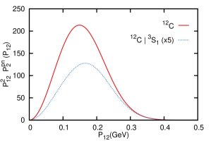
Figure 8: (Color online) The pn c.m. distribution $P_{12}^{2}P_{2}^{pn}\left(P_{12}\right)$ and $P_{12}^{2}P_{2}^{pn}\left(P_{12}|^{3}S_{1}\right)=P_{12}^{2}F^{pn}\left(P_{12}\right)$ for ¹²C. The calculations are performed with HO single-particle states and adopt the normalization convention $\int dP_{12}\;P_{12}^{2}P_{2}^{pn}\left(P_{12}\right)=NZ$.

To estimate the c.m. correction factor we have performed MC simulations of pn knockout with and without inclusion of the c.m. motion. This amounts to drawing the c.m. momentum from $F^{pn}(P_{12})=\delta(P_{12})$ and $F^{pn}(P_{12})\sim e^{-\frac{P_{12}^{2}}{2\sigma_{c.m.}^{2}}}$, where $\sigma_{c.m.}$ is the $A$ dependent width. For $1.5\leq x_{B}\leq 2$, the initial momentum distribution of the correlated pair is given by correlated part of the two-body momentum distribution $n_{2}^{(1)}(k_{12},P_{12})$. The Eq. (23) states that the $n_{2}^{(1)}\left(k_{12},P_{12}\right)$ can be considered universal. As illustrated in Fig. 1 one has ${n}_{D}\left(k_{12}\right)\sim\left|f_{t\tau}(k_{12})\right|^{2}$. As the relative momentum distribution is approximately proportional to the tensor correlation function, we draw $k_{12}$ from the distribution $k_{12}^{2}|f_{t\tau}(k_{12})|^{2}$. Energy conservation reads

$$(q+p_{A}-p_{A-2}-p_{s})^{2}=p_{f}^{2}=m_{N}^{2},$$ (51)

where $q(\omega,\vec{q})$, $p_{A}(M_{A},\vec{0})$ and $p_{A-2}(E_{A-2},-(\vec{p}_{s}+\vec{p}_{m}))$ are the four-momenta of the virtual photon, target nucleus and residual $A-2$ system, respectively. The virtual photon interacts with one of the nucleons, resulting in a fast nucleon $p_{f}(E_{f},\vec{p}_{f})$ with $\vec{p}_{f}=\vec{p}_{m}+\vec{q}$ and a slow nucleon $p_{s}(E_{s},\vec{p}_{s})$. With the aid of Eq. (51), one can calculate the $x_{B}$-distribution of the simulated events. We apply the kinematics of the Jefferson Lab (JLab) experiment E02-019 Fomin et al. (2012): $\epsilon_{i}=$5.766\text{\,}\mathrm{GeV}$$ and $\theta_{e}=$18\text{\,}\mathrm{\SIUnitSymbolDegree}$$. The average $<Q^{2}>$ of the generated events (including c.m. motion) in the $x_{B}$ region of interest is 2.7 GeV². This value, which is $A$-independent, agrees with the one quoted in Ref. Fomin et al. (2012).

The results of our simulations are summarized in Figs. 9 and 10. Fig. 9 shows the $x_{B}-k_{12}$ scatter plot of $10^{6}$ simulated events with and without inclusion of c.m. motion for ¹²C. In both situations the mass difference between inital and final state causes a small shift to lower $x_{B}$ compared to the deuteron case. Second, we observe considerable shifts in the distribution of the events in the $(k_{12},x_{B})$ plane due to c.m. motion. In Fig. 10, one can observe how c.m. motion considerably increases the number of events with $1.5\leq x_{B}\leq 2$. The impact of the c.m. corrections increases with growing $x_{B}$. Experimentally, the $a_{2}(A/D)$ coefficient is determined by integrating data for $1.5\leq x_{B}\leq 1.85$. We estimate the c.m. correction factor by the ratio

$$\frac{\textrm{\# simulated events with inclusion of c.m. motion}}{\textrm{\# simulated events without inclusion of c.m. motion}}\;.$$ (52)

in this $x_{B}$ region. The resulting correction factor for several nuclei is contained in Table 1. We performed the simulations with the three different correlation functions $f_{t\tau}$ in Fig. 1. The dependence of the result on the choice of correlation function is represented by the error of the c.m. correction factor.

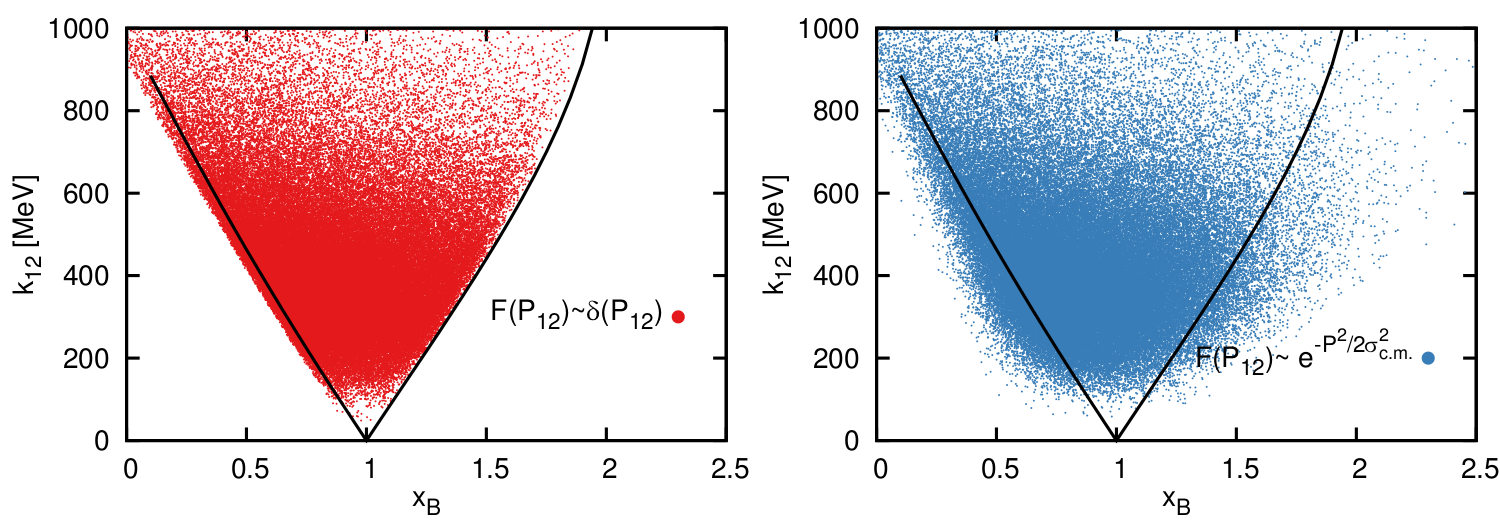
Figure 9: (Color online) The $k_{12}-x_{B}$ scatter plot of ¹²C$(e,e^{\prime}pn)$ MC simulations with ($F(P_{12})\sim e^{-\frac{P_{12}^{2}}{2\sigma_{c.m.}^{2}}}$ ) and without ($F(P_{12})\sim\delta(P_{12})$) inclusion of c.m. motion. For the sake of comparison the solid line shows the minimum relative momentum $k_{12}^{min}$ for $Q^{2}=$2.7\text{\,}{\mathrm{GeV}}^{2}$$ in the deuteron.

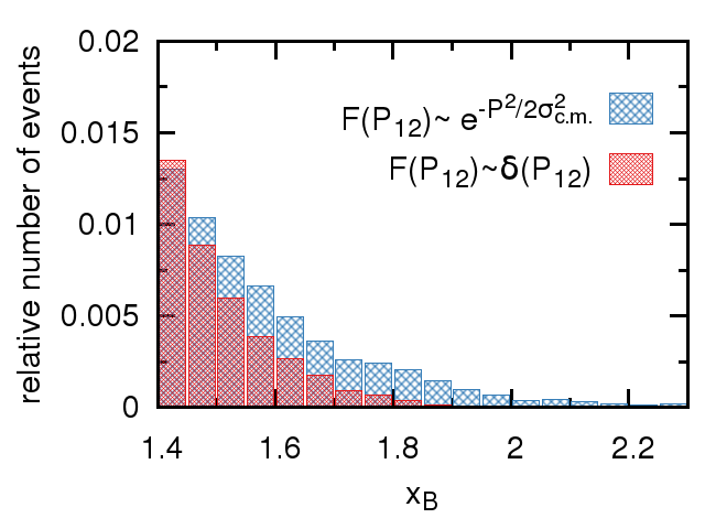
Figure 10: (Color online) Histogram of the $x_{B}$ distribution of ¹²C$(e,e^{\prime}pn)$ MC simulations with ($F(P_{12})\sim e^{-\frac{P_{12}^{2}}{2\sigma_{c.m.}^{2}}}$ ) and without ($F(P_{12})\sim\delta(P_{12})$) inclusion of c.m. motion. The kinematics is the one of the JLab experiment E02-019 Fomin et al. (2012): $\epsilon_{i}=$5.766\text{\,}\mathrm{GeV}$$ and $\theta_{e}=$18\text{\,}\mathrm{\SIUnitSymbolDegree}$$.

A	$\sigma_{c.m.}$	c.m. correction factor
12C	$115$ MeV	$1.64\pm 0.23$
56Fe	$128$ MeV	$1.70\pm 0.27$
208Pb	$141$ MeV	$1.71\pm 0.29$

Table 1: The second column gives the width of the c.m. distribution of correlated pn pairs. The third column provides the computed c.m. correction factor. The errors represent the dependence on the choice of correlation function.

Fig. 3 quantifies the fraction of all possible pn pairs which are prone to SRC relative to the total amount of possible pn pair combinations. In our picture one has $N_{pn(S=1)}=1$ for D. This means that we do interpret the $l_{12}=0$ component of the deuteron wave function as the IPM part which receives large corrections from tensor SRC. The per nucleon probability for a pn SRC relative to the deuterium can be defined as

$$\frac{2}{N+Z}\frac{N_{pn(S=1)}(A,Z)}{N_{pn(S=1)}(A=2,Z=1)}=\frac{2}{A}{N_{pn(S=1)}(A,Z)}\;.$$ (53)

Similar expressions hold for the per nucleon pp SRC and the per nucleon nn SRC

$$\frac{2}{Z}{N_{pp(S=0)}(A,Z)}\quad\quad\frac{2}{N}{N_{nn(S=0)}(A,Z)}\;.$$ (54)

The results of the per nucleon probabilities are collected in Fig. 11. Relative to ²H, the per nucleon probability of pn SRC are 2.20, 3.63, 4.73 times larger for Carbon, Iron, Gold. Along similar lines, relative to the “free” pp system the per nucleon probability of pp SRC are 1.39, 2.34, 3.11 times larger for Carbon, Iron, Gold.

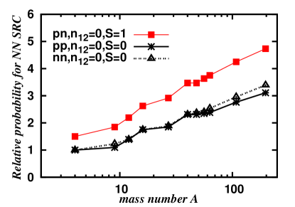
Figure 11: The mass dependence of the per nucleon probability for pn SRC relative to the deuterium.

In Fig. 12 we compare our predictions computed with the aid of the Eq.  (49) with the extracted values of $a_{2}(A/D)$. We have opted to correct the predicted $a_{2}$ coefficients and not the data for c.m. motion. We stress that the c.m. correction factor cannot be computed in a model-independent fashion. For light nuclei our predictions tend to underestimate the measured $a_{2}$. This could be attributed to the lack of long-range clustering effects in the adopted wave functions. Indeed, it was pointed out in Ref. Hirai et al. (2011) that the high-density cluster components in the wave functions are an important source of correlation effects beyond the mean-field approach. For heavy nuclei our predictions for the relative SRC probability per nucleon do not saturate as much as the data seem to indicate. In Ref. Frankfurt et al. (2008) the authors estimated the mass dependence of $a_{2}$ by means of an expression of the type $a_{2}\sim\int d^{3}\vec{r}\rho^{2}_{\text{MF}}(\vec{r})$. Using Skyrme Hartree-Fock densities $\rho_{\text{MF}}(\vec{r})$ a power-law of $A^{0.12}$ emerged. After normalizing to the measured value for $a_{2}(^{12}$C$/D)$ the predicted power-low dependence agrees nicely with the data.

We stress that final-state interactions (FSI) represent another source of corrections which may induce an additional $A$-dependent correction to the data. FSI of the outgoing nucleons with the residual spectator nucleons, could shift part of the signal strength out of the cuts applied to the experimental phase space (or likewise move strength in) and decrease (or increase) the measured cross section and the corresponding $a_{2}$ coefficient.

In Fig. 13 we display the magnitude of the EMC effect, quantified by means of $-\frac{dR}{dx_{B}}$ versus our predictions for the quantity $\frac{2}{A}N_{pn(S=1)}$ or, the ”per nucleon probability for pn SRC relative to the deuteron”. We stress that the numbers which one finds on the x-axis are the results of parameter-free calculations. We consider the ”per nucleon probability for pn SRC relative to the deuteron” as a measure for the magnitude of the proton-neutron SRC in a given nucleus. Obviously, there is a nice linear relationship between the quantity which we propose as a per nucleon measure for the magnitude of the SRC and the magnitude of the EMC effect.

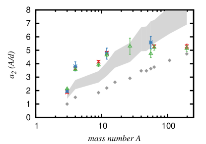
Figure 12: (Color online) The computed values for the $a_{2}(A/D)$ for various nuclei. The data are from Refs. Egiyan et al. (2006); Fomin et al. (2012); Arrington et al. (2012a). The shaded region is the prediction after correcting the computed values of $a_{2}(A/D)$ for the c.m. motion of the pair. The correction factor are determined by linear interpolation of the factors listed in Table 1. The width of the shaded area is determined by the error of the c.m. correction factors.

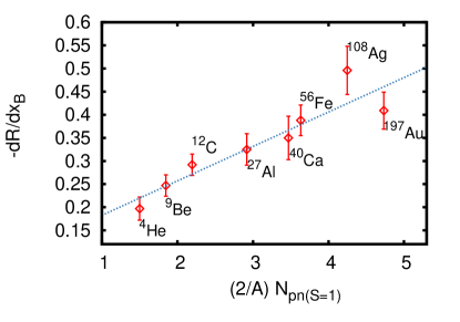
Figure 13: The magnitude of the EMC effect versus the computed per nucleon number of correlated pn pairs. The data are from the analysis presented in Refs. Seely et al. (2009); Gomez et al. (1994); Arrington et al. (2012a). The fitted line obeys the equation $-\frac{dR}{dx_{B}}=(0.108\pm 0.028)+\frac{2}{A}N_{pn(S=1)}\cdot(0.074\pm 0.010)$.

III.3 Three-body correlations

The measurements of Refs. Egiyan et al. (2006); Fomin et al. (2012) indicate that the ratio of the inclusive cross sections

$$\frac{\sigma^{A}\left(x_{B},Q^{2}\right)}{\sigma^{{}^{3}\textrm{He}}\left(x_{B},Q^{2}\right)}\;,$$ (55)

approximately scales for $2.25\lesssim x_{B}\lesssim 3.0$. Along similar lines as those used in quantifying the 2N SRC in Sec. III.2, it has been suggested Egiyan et al. (2006) to parameterize the inclusive $A(e,e^{\prime})$ cross section in the following form

$$\sigma^{A}\left(2.25\lesssim x_{B}\lesssim 3,Q^{2}\right)=\frac{A}{3}a_{3}\left({A}/{{}^{3}\textrm{He}}\right){\sigma_{3}\left(x_{B},Q^{2}\right)}\;,$$ (56)

where ${\sigma_{3}\left(x_{B},Q^{2}\right)}$ is the cross section for scattering from a correlated 3N cluster which is once again assumed to be $A$ independent. Inserting Eq. (56) into Eq. (55), one obtains

$$a_{3}\left({A}/^{3}\textrm{He}\right)=\frac{3}{A}\frac{\sigma^{A}\left(x_{B},Q^{2}\right)}{\sigma^{{}^{3}\textrm{He}}\left(x_{B},Q^{2}\right)}\;\;\left(2.25\lesssim x_{B}\lesssim 3.0\right)\;.$$ (57)

Notice that in the kinematic regime where 3N correlations are expected to dominate $\left(2.25\lesssim x_{B}\right)$ the experimental situation is unsettled. For example, the recently measured $a_{3}(^{4}$He/³He) ratios Fomin et al. (2012) are significantly larger than those reported in Ref. Egiyan et al. (2006).

Similar to the per nucleon pn SRC of Eq. (53) we define the per nucleon probability for a ppn SRC relative to ³He as

$$\frac{3}{A}\frac{N_{ppn}\left(A,Z\right)}{N_{ppn}\left(A=3,Z=2\right)}=\frac{3}{A}N_{ppn}\left(A,Z\right),$$ (58)

where we used the fact that $N_{ppn}\left(A=3,Z=2\right)=1$ in our framework. The results of the per nucleon probability of ppn SRC are collected in Figure 14.

The quantity of Eq. (58) can be linked to $a_{3}(A/^{3}\textrm{He})$ under the condition that corrections stemming from c.m. motion of the correlated ppn triples, FSI effects, $\ldots$ are small. Under those idealized conditions one would have

$$a_{3}(A,^{3}\textrm{He})\approx\frac{3}{A}N_{ppn}(A,Z)\;.$$ (59)

In the naive assumption that all 3N pairs contribute to the $a_{3}(A/^{3}\textrm{He})$ ratio, one expects an $A^{2}$ dependency. We suggest that only ppn triples in a “close” configuration contribute and we count the number of SRC triples with the aid of the Eq. (40). The ppn contributions will be larger than the pnn ones due to the magnitude of the electromagnetic coupling. Correlated triples should have at least one pn pair due to the dominant character of the tensor component. In Fig. 14 we show the predictions for the $a_{3}(A/{{}^{3}\textrm{He}})$ coefficient as computed with the Eq.  (59) and compare it to the data. We stress that the experimental situation is largely unsettled and that neither the data nor the theoretical calculations have been corrected for c.m. motion and FSI effects. For Helium and Carbon our predictions are in line with the experimental value. For Iron the prediction is about a factor of two larger than the experimentally determined ratio of cross sections. Our parameter-free calculations reproduce the fact that the mass dependence is much softer than the $A^{2}$ dependence that one would expect on naive grounds.

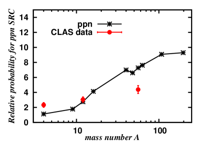
Figure 14: The mass dependence of the per nucleon probability for ppn SRC relative to ³He. We stress that neither the data nor the theoretical calculations have been corrected for c.m. motion and FSI effects. The data are from Ref. Egiyan et al. (2006).

IV Conclusion

We have provided arguments that the mass dependence of the magnitude of the NN and NNN correlations can be captured by some approximate principles. Our method is based on the assumption that correlation operators generate the correlated part of the nuclear wave function from that part of the mean-field wave function where two nucleons are “sufficiently close”. This translates to computing those parts of the two-nucleon and three-nucleon wave functions with zero relative orbital momentum in order to identify short-range correlated pairs and triples.

We have calculated the number of pn, pp and nn $l_{12}=0$ SRC pairs and studied their mass and isospin dependence. The $A$ dependence of the magnitude of the pp, nn, and pn SRC manifests itself in a power-law dependence. We found a significant higher per nucleon SRC probability for pn pairs than for pp and for nn. To connect the computed number of SRC pairs to the measured $a_{2}\left(A/\textrm{D}\right)$ corrections are in order. Published experimental data include the radiation and Coulomb corrections. The correction factor stemming from final-state interactions and from the c.m. motion of the correlated pair, however, is far from established. We proposed a method to estimate the c.m. correction factor based on general properties of nucleon momentum distributions. Using Monte Carlo simulation we find a correction factor of about $1.7\pm 0.3$. Our model calculations for $a_{2}$ are of the right order of magnitude and capture the $A$-dependence qualitatively. For small $A$ our predictions underestimate the data, while we do not find the same degree of saturation for high $A$ that the (scarce) data seem to suggest.

To compute the number of 3N SRC in a nucleus, we count the ppn states with three nucleons which are close. We have quantified the number of 3N SRC and provided predictions for the measured $a_{3}\left(A/^{3}\textrm{He}\right)$ coefficients. Our model calculations for the $a_{3}$ are of the same order of magnitude as the (scarce) data but overestimate the ⁵⁶Fe data point. In this comparison no corrections for c.m. motion and FSI effects have been made and it remains to be studied in how far they can blur the connection between inclusive electron-scattering data and the SRC information. We find a linear relationship between the magnitude of the EMC effect and the computed per nucleon number of SRC pn pairs. This may indicate that the EMC effect is (partly) driven by local nuclear dynamics (fluctuations in the nuclear densities), and that the number of pn SRC pairs serves as a measure for the magnitude of this effect.

Acknowledgments

The computational resources (Stevin Supercomputer Infrastructure) and services used in this work were provided by Ghent University, the Hercules Foundation and the Flemish Government – department EWI. This work is supported by the Research Foundation Flanders.

References

- Broniowski and Rybczynski (2010) W. Broniowski and M. Rybczynski, Phys. Rev. C 81 (2010).
- Blunden and Sick (2005) P. G. Blunden and I. Sick, Phys. Rev. C 72, 057601 (2005).
- Engel et al. (2011) J. Engel, J. Carlson, and R. Wiringa, Phys. Rev. C 83, 034317 (2011), eprint 1101.0554.
- Alvioli and Strikman (2011) M. Alvioli and M. Strikman, Phys. Rev. C 83, 044905 (2011), eprint 1008.2328.
- Cosyn et al. (2008) W. Cosyn, M. C. Martinez, and J. Ryckebusch, Phys. Rev. C 77, 034602 (2008), eprint 0710.4837.
- Aubert et al. (1983) J. Aubert et al. (European Muon Collaboration), Phys.Lett. B123, 275 (1983).
- Seely et al. (2009) J. Seely, A. Daniel, D. Gaskell, J. Arrington, N. Fomin, et al., Phys.Rev.Lett. 103, 202301 (2009), eprint 0904.4448.
- Day et al. (1987) D. Day, J. Mccarthy, Z. Meziani, R. Minehart, R. Sealock, et al., Phys. Rev. Lett. 59, 427 (1987).
- Egiyan et al. (2006) K. S. Egiyan, N. B. Dashyan, M. M. Sargsian, M. I. Strikman, L. B. Weinstein, G. Adams, P. Ambrozewicz, M. Anghinolfi, B. Asavapibhop, G. Asryan, et al. (CLAS Collaboration), Phys. Rev. Lett. 96, 082501 (2006).
- Fomin et al. (2012) N. Fomin, J. Arrington, R. Asaturyan, F. Benmokhtar, W. Boeglin, P. Bosted, A. Bruell, M. H. S. Bukhari, M. E. Christy, E. Chudakov, et al., Phys. Rev. Lett. 108, 092502 (2012).
- Frankfurt et al. (2008) L. Frankfurt, M. Sargsian, and M. Strikman, Int. J. Mod. Phys. A23, 2991 (2008), eprint 0806.4412.
- Weinstein et al. (2011) L. Weinstein, E. Piasetzky, D. Higinbotham, J. Gomez, O. Hen, et al., Phys. Rev. Lett. 106, 052301 (2011), eprint 1009.5666.
- Hen et al. (2012) O. Hen, E. Piasetzky, and L. Weinstein, Phys. Rev. C 85, 047301 (2012), eprint 1202.3452.
- Arrington et al. (2012a) J. Arrington, A. Daniel, D. Day, N. Fomin, D. Gaskell, et al. (2012a), eprint 1206.6343.
- Schiavilla et al. (2007) R. Schiavilla, R. B. Wiringa, S. C. Pieper, and J. Carlson, Phys. Rev. Lett. 98, 132501 (2007), eprint nucl-th/0611037.
- Wiringa et al. (2008) R. Wiringa, R. Schiavilla, S. C. Pieper, and J. Carlson, Phys. Rev. C 78, 021001 (2008), eprint 0806.1718.
- Feldmeier et al. (2011) H. Feldmeier, W. Horiuchi, T. Neff, and Y. Suzuki, Phys. Rev. C 84, 054003 (2011), eprint 1107.4956.
- Alvioli et al. (2008) M. Alvioli, C. Ciofi degli Atti, and H. Morita, Phys. Rev. Lett. 100, 162503 (2008).
- Bisconti et al. (2006) C. Bisconti, F. Arias de Saavedra, and G. Co’, Phys. Rev. C 73, 054304 (2006), eprint nucl-th/0601081.
- Bisconti et al. (2007) C. Bisconti, F. Arias de Saavedra, and G. Co, Phys. Rev. C 75, 054302 (2007), eprint nucl-th/0702061.
- Vanhalst et al. (2011) M. Vanhalst, W. Cosyn, and J. Ryckebusch, Phys. Rev. C 84, 031302 (2011), eprint 1105.1038.
- Arrington et al. (2012b) J. Arrington, D. Higinbotham, G. Rosner, and M. Sargsian, Prog.Part.Nucl.Phys. 67, 898 (2012b), eprint 1104.1196.
- Shneor et al. (2007) R. Shneor, P. Monaghan, R. Subedi, B. D. Anderson, K. Aniol, J. Annand, J. Arrington, H. Benaoum, F. Benmokhtar, P. Bertin, et al. (Jefferson Lab Hall A Collaboration), Phys. Rev. Lett. 99, 072501 (pages 5) (2007).
- Ryckebusch (2001) J. Ryckebusch, Phys. Rev. C 64, 044607 (2001).
- Ryckebusch (1996) J. Ryckebusch, Phys. Lett. B383, 1 (1996), eprint nucl-th/9605043.
- Alvioli et al. (2012) M. Alvioli, C. Ciofi degli Atti, L. P. Kaptari, C. B. Mezzetti, H. Morita, and S. Scopetta, Phys. Rev. C 85, 021001 (2012).
- Roth et al. (2010) R. Roth, T. Neff, and H. Feldmeier, Prog. Part. Nucl. Phys. 65, 50 (2010), eprint 1003.3624.
- Pieper et al. (1992) S. C. Pieper, R. B. Wiringa, and V. Pandharipande, Phys. Rev. C 46, 1741 (1992).
- Arias de Saavedra et al. (1996) F. Arias de Saavedra, G. Co’, A. Fabrocini, and S. Fantoni, Nucl. Phys. A605, 359 (1996), eprint nucl-th/9604013.
- Gearheart (1994) C. Gearheart, Ph.D. thesis, Washington University, St. Louis (1994).
- Alvioli et al. (2005) M. Alvioli, C. Ciofi degli Atti, and H. Morita, Phys. Rev. C 72, 054310 (2005), eprint nucl-th/0506054.
- Lacombe et al. (1980) M. Lacombe, B. Loiseau, J. M. Richard, R. V. Mau, J. Côté, P. Pirès, and R. de Tourreil, Phys. Rev. C 21, 861 (1980).
- Lacombe et al. (1981) M. Lacombe, B. Loiseau, R. Mau, J. Côté, P. Pirés, and R. de Tourreil, Physics Letters B 101, 139 (1981), ISSN 0370-2693.
- Frankfurt and Strikman (1988) L. Frankfurt and M. Strikman, Phys. Rep. 160, 235 (1988).
- Ciofi degli Atti and Simula (1996) C. Ciofi degli Atti and S. Simula, Phys. Rev. C 53, 1689 (1996), eprint nucl-th/9507024.
- Janssen et al. (2000) S. Janssen, J. Ryckebusch, W. Van Nespen, and D. Debruyne, Nucl. Phys. A 672, 285 (2000).
- Iodice et al. (2007) M. Iodice, E. Cisbani, R. De Leo, S. Frullani, F. Garibaldi, et al., Phys.Lett. B653, 392 (2007), eprint nucl-ex/0703007.
- Starink et al. (2000) R. Starink, M. van Batenburg, E. Cisbani, W. Dickhoff, S. Frullani, F. Garibaldi, C. Giusti, D. Groep, P. Heimberg, W. Hesselink, et al., Phys. Lett. B 474, 33 (2000).
- Ryckebusch and Van Nespen (2004) J. Ryckebusch and W. Van Nespen, Eur. Phys. J. A 20, 435 (2004).
- Middleton et al. (2007) D. Middleton, J. Annand, C. Barbieri, P. Barneo, P. Bartsch, et al., Eur. Phys. J. A 29, 261 (2007), eprint nucl-ex/0701053.
- Ryckebusch et al. (2000) J. Ryckebusch, S. Janssen, W. Van Nespen, and D. Debruyne, Phys. Rev. C 61, 021603R (2000).
- Barbieri et al. (2004) C. Barbieri, C. Giusti, F. Pacati, and W. Dickhoff, Phys. Rev. C 70, 014606 (2004), eprint nucl-th/0402081.
- Subedi et al. (2008) R. Subedi, R. Shneor, P. Monaghan, B. Anderson, K. Aniol, et al., Science 320, 1476 (2008), eprint 0908.1514.
- Baghdasaryan et al. (2010) H. Baghdasaryan, L. B. Weinstein, J. M. Laget, K. P. Adhikari, M. Aghasyan, M. Amarian, M. Anghinolfi, H. Avakian, J. Ball, M. Battaglieri, et al. (CLAS Collaboration), Phys. Rev. Lett. 105, 222501 (2010).
- Moshinsky and Smirnov (1996) M. Moshinsky and Y. F. Smirnov, The harmonic oscillator in modern physics (Informa HealthCare, Amsterdam, 1996).
- Sargsian (2001) M. M. Sargsian, Int.J.Mod.Phys. E10, 405 (2001), eprint nucl-th/0110053.
- Frankfurt et al. (1993) L. L. Frankfurt, M. I. Strikman, D. B. Day, and M. Sargsyan, Phys. Rev. C 48, 2451 (1993).
- Benhar et al. (1995) O. Benhar, A. Fabrocini, S. Fantoni, and I. Sick, Phys.Lett. B343, 47 (1995).
- Benhar et al. (1994) O. Benhar, A. Fabrocini, S. Fantoni, and I. Sick, Nucl.Phys. A579, 493 (1994).
- Sick et al. (1994) I. Sick, S. Fantoni, A. Fabrocini, and O. Benhar, Phys.Lett. B323, 267 (1994).
- Ciofi degli Atti and Simula (1994) C. Ciofi degli Atti and S. Simula, Phys.Lett. B325, 276 (1994), eprint nucl-th/9403001.
- Piasetzky et al. (2006) E. Piasetzky, M. Sargsian, L. Frankfurt, M. Strikman, and J. Watson, Phys. Rev. Lett. 97, 162504 (2006), eprint nucl-th/0604012.
- Blomqvist et al. (1998) K. I. Blomqvist et al., Phys. Lett. B421, 71 (1998).
- Hirai et al. (2011) M. Hirai, S. Kumano, K. Saito, and T. Watanabe, Phys. Rev. C 83, 035202 (2011).
- Gomez et al. (1994) J. Gomez, R. G. Arnold, P. E. Bosted, C. C. Chang, A. T. Katramatou, G. G. Petratos, A. A. Rahbar, S. E. Rock, A. F. Sill, Z. M. Szalata, et al., Phys. Rev. D 49, 4348 (1994), URL http://link.aps.org/doi/10.1103/PhysRevD.49.4348.