We do not live in the $\mn@boldsymbol{R_{\mathrm{h}}=c\,t}$ universe

Abstract

We analyse the possibility that our Universe could be described by the model recently proposed by Melia & Shevchuk (2012), where the Hubble scale $R_{\mathrm{h}}=c/H$ is at all times equal to the distance $c\,t$ that light has travelled since the Big Bang. In such a model, the scale factor is proportional to cosmic time and there is neither acceleration nor deceleration of the expansion. We first point out problems with the very foundations of the model and its consequences for the evolution of the Universe. Next, we compare predictions of the model with observational data. As probes of the expansion we use distance data of supernovae type Ia, as well as Hubble rate data obtained from cosmic chronometers and radial baryon acoustic oscillations. We analyse the redshift evolution of the Hubble parameter and its redshift derivatives, together with the so-called $\mathcal{O}_{\mathrm{m}}$ diagnostic and the deceleration parameter. To reliably estimate smooth functions and their derivatives from discrete data, we use the recently developed Gaussian Processes in Python package (GaPP). Our general conclusion is that the discussed model is strongly disfavoured by observations, especially at low redshifts ($z\la 0.5$). In particular, it predicts specific constant values for the deceleration parameter and for redshift derivatives of the Hubble parameter, which is ruled out by the data.

1 Introduction

The fact that the Universe is currently undergoing a phase of accelerated expansion has been known for more than a decade. The first evidence came from observations of distant supernovae type Ia (SNeIa) by Riess et al. (1998) and Perlmutter et al. (1999). This result has been confirmed by various observations, e.g. of the cosmic microwave background and its angular power spectrum (Komatsu et al., 2011), baryon acoustic oscillations (BAO, e.g. Percival et al. 2010) and SNeIa (Suzuki et al., 2012); see Weinberg et al. (2012) for a general review.

However, the picture that emerges based on these and multiple other observations is far from being theoretically understood. In a homogeneous and isotropic Universe and assuming general relativity to be correct on cosmological scales, one needs some form of dark energy as the driving force of the observed acceleration. The simplest model that is consistent with observations is the Lambda-Cold Dark Matter ($\Lambda$CDM) – a model where the dark energy has a constant energy density.

This theory has no physical understanding at the moment and in recent years considerable effort has been devoted to develop and test alternative explanations of the accelerated cosmic expansion. These efforts include dark energy models with an equation of state that is more complex than that of $\Lambda$CDM, inhomogeneous models and theories assuming deviations from general relativity, known under the collective name of modified gravity [see Copeland et al. (2006) for a review].

2 The $\mn@boldsymbol{R}$$\mn@boldsymbol{{}_{\mathrm{h}}=c\,t}$ model and its problems

In a recent paper, Melia & Shevchuk (2012, hereafter MS12) have offered a qualitatively different cosmological model, which was meant to solve some of the problems of the $\Lambda$CDM. Namely, they used the general relativistic framework of Friedman-Lemaître models with the Robertson-Walker metric and, having applied the Weyl postulate, proposed a model in which there is neither acceleration nor deceleration either now or in the past. It is claimed that this is the only viable cosmological model as all other models allegedly violate the Weyl postulate. In this eternally coasting model, the scale factor grows linearly with time. Additionally, the MS12 model predicts the Hubble parameter to be always exactly equal to the inverse of the age of the Universe, i.e. $H(z)=t^{-1}(z)$, where $t$ is the cosmic time and $z$ is the cosmological redshift. MS12 argue that the best-fit (concordance) cosmological model only mimics the real underlying one, which they call the $R_{h}=c\,t$ Universe (see also Melia 2012 for a more popular description). For simplicity of notation, it will be referred to as the ‘$H\,t=1$ model’ hereunder.

As one of the motivations to introduce their model, MS12 point out that the currently observed coincidence that $R_{\mathrm{h}}=c\,t_{0}$ (where $t_{0}$ denotes the current age of the Universe) is possible within $\Lambda$CDM models only once, i.e. exactly now. On the other hand, as they argue, such an equality [i.e. $R_{\mathrm{h}}=c/H(t)$] is obtained for all times in a straightforward manner if one applies the Weyl postulate when constructing the space-time metric.

MS12 start by defining the gravitational radius (better known as Schwarzschild radius) as

$$R_{\mathrm{h}}\equiv\frac{2\,GM(R_{\mathrm{h}})}{c^{2}}$$ (1)

[equation (8) of MS12], where $M(R_{\mathrm{h}})$ is the mass enclosed within $R_{\mathrm{h}}$

$$M(R_{\mathrm{h}})=V_{\mathrm{prop}}\frac{\rho(t)}{c^{2}}\;,$$ (2)

and

$$V_{\mathrm{prop}}=\frac{4\pi}{3}R_{\mathrm{h}}^{3}$$ (3)

is the proper volume, defined by MS12 such that the comoving density of particles within it remains fixed as the Universe expands. Here, $\rho(t)$ denotes the energy density.

MS12 later argue that the gravitational radius is equivalent to the Hubble radius. We doubt that the definition of the Schwarzschild radius makes sense on such large scales. One of the crucial assumptions in deriving the Schwarzschild radius is a static space-time. This condition is certainly not true when expanding regions are considered. Nevertheless we will continue to follow the argumentation given in MS12 and point out another problem in their theory. This is additional to what has been described in two earlier papers dealing with some flaws of the MS12 model (van Oirschot et al., 2010; Lewis & van Oirschot, 2012).

Combining the Equations (1)–(3) with the Friedmann equation for a flat Universe

$$H^{2}(t)=\frac{8\pi G}{c^{2}}\rho(t)$$ (4)

one finds

$$R_{\mathrm{h}}(t)=\frac{c}{H(t)}\;,$$ (5)

which is the usual definition of the Hubble radius. Using $R_{\mathrm{h}}(t)=a(t)r_{\mathrm{h}}$ and $H(t)=\dot{a}(t)/a(t)$, we find for the comoving Hubble radius $r_{\mathrm{h}}$:

$$r_{\mathrm{h}}=\frac{c}{\dot{a}(t)}$$ (6)

The next step of MS12 argumentation contains another flaw. They claim that $r_{\mathrm{h}}$ needs to be constant because ‘otherwise $V_{\mathrm{prop}}$ would not represent the volume within which the particle density is constant in the comoving frame’. This argument is, however, not convincing. In a homogeneous Universe, the size of a volume – and thus the value of $r_{\mathrm{h}}$ – does not affect the particle density within that volume. Therefore, there is no reason to assume that $r_{\mathrm{h}}$ is constant. Consequently, it can neither be implied that $\dot{a}$ is constant, nor that the scale factor is linear in time, nor that the equation of state (EOS) $w=-1/3$ (see hereunder).

If the argumentation of MS12 were correct, that would have some odd consequences for the evolution of the Universe, which we will examine in the following. Being a special case of a power-law cosmology (see Kumar 2012 for a recent discussion, and references therein), in which the scale factor $a(t)\propto t^{\alpha}$, this model has a simple mathematical form. However, it is arguably not more plausible from the astrophysical point of view than the standard $\Lambda$CDM. Firstly, as can be seen in equation (6), a constant $r_{\mathrm{h}}$ would imply that $\dot{a}$ is constant and thus the deceleration parameter equal to zero, $q(z)\equiv 0$. Secondly, from Equations (1)–(3), it follows that $R_{\mathrm{h}}\propto M(R_{\mathrm{h}})\propto\rho R_{\mathrm{h}}^{3}$, so we get that $\rho R_{\mathrm{h}}^{2}=\mathrm{const}$ at all times. In combination with $R_{\mathrm{h}}(t)=a(t)r_{\mathrm{h}}$ and assuming $r_{\mathrm{h}}$ to be constant, this leads directly to the following scaling for energy density, which must hold in the $H\,t=1$ model:

$$[H\,t=1]\qquad\rho(t)\propto a(t)^{-2}\;.$$ (7)

It is easy to check that it is equivalent to require the EOS to be $w=p/\rho\equiv-1/3$, as discussed in MS12.

Recall that according to MS12 all other homogeneous and isotropic cosmological models are ruled out due to (incorrect, as we believe) theoretical reasoning. These models would not even have consistent general relativistic solution. Thus, a homogeneous dust Universe would not have a general relativistic solution because it has $w=0$. Neither would inflation be possible. The contents of the Universe would need to be fine-tuned in such a way that the overall effective EOS equals $-1/3$ at all times. Such a high degree of fine-tuning is very hard to achieve. Another problem is that the growth of fluctuations in the $H\,t=1$ model is driven by a (negative) pressure term, which looks the same no matter the perturbation length. It is thus somewhat unclear how the large-scale structure would emerge within this model.

Finally, however, neither simplicity nor plausibility are the decisive factors for a cosmological model to be accepted as a proper description of the physical Universe. The condition under which we can treat the model as valid, or at least a good approximation to reality, is that it has successfully passed confrontations with multiple observational data. Not all tests, applicable elsewhere, can be currently performed within the $H\,t=1$ model, owing to the lack of theoretical framework in some domains. For example, the perturbation theory of gravitational instability, so successfully applied in $\Lambda$CDM (e.g. Davis et al. 2011; Nusser & Davis 2011; Bilicki et al. 2011 for recent results), could not be used in the discussed model. As shown in MS12, the growth of density fluctuations is qualitatively different there from the standard cosmology and its quantitative details still await investigation. However, as we will show below, such analyses might already be no more than of academic interest, as the model can be effectively falsified with other, simpler methods. Examining the consequences of the $H\,t=1$ model for the expansion history of the Universe and its various indicators leads us to conclude that the MS12 model is strongly disfavoured by observations.

3 Supernova type Ia data

One of the most important tests of the cosmic expansion history consists in comparing redshifts and distances of far-away objects with predictions of particular models. For example, in case of SNeIa, the quantity used is the luminosity distance, derived by lightcurve fitting from observed peak luminosities and analysed afterwards as a function of cosmological redshift.

Assuming spatial flatness, as was done in MS12, the luminosity distance in $\Lambda$CDM models with a cosmological constant (dark energy equation of state $w=-1$) is given by

$$d_{\mathrm{L}}=\frac{c}{H_{0}}(1+z)\int\limits_{0}^{z}{\frac{\mathrm{d}\zeta}{\left[\Omega_{\mathrm{m}}(1+\zeta)^{3}+\Omega_{\Lambda}\right]^{1/2}}}\;.$$ (8)

In the $H\,t=1$ model, it takes the following closed-form expression:

$$[H\,t=1]\qquad d_{\mathrm{L}}=R_{\mathrm{h}}(t_{0})(1+z)\ln(1+z)\;,$$ (9)

where $R_{\mathrm{h}}(t_{0})=c/H_{0}$. In principle, comparing this curve with available data could be used to directly verify the validity of the model. Indeed, MS12 discuss it shortly and even admit that this form of the luminosity distance does not fit the current sample of Type Ia supernovae (see e.g. Riess et al. 2004). They however argue that this discrepancy is present only for redshifts of $\sim 0.5$, where – as they claim – different SNeIa catalogues are inconsistent with each other. In particular, they refer to the fact that analyses made by different authors do not yield a consistent value of the redshift $z_{\mathrm{acc}}$ at which, within $\Lambda$CDM, there was a transition from past deceleration to currently observed acceleration of the universal expansion.

Putting these issues aside, we only mention a known caveat related to using luminosity distances of SNeIa, or their more observer-friendly variant, distance moduli, as direct probes of cosmic expansion. When using the SALT light-curve fitter (Guy et al., 2005, 2007) some nuisance parameters that are needed to determine the distance moduli from the raw data, are fitted simultaneously with the cosmological parameters. Thus, the distance muduli in the data sets are somewhat model-dependent. While the MLCS2k2 light-curve fitter (Jha et al., 2007) avoids these issues, other systematics are present (e.g. the reddening parameter $R_{V}$ has to be fixed by hand). Thus, although both types of light-curve fitters have some systematics, these are of different nature. So when accelerated expansion is found independently by using different fitters, this should be a fairly robust result.

When discussing the luminosity distance, MS12 question the validity of introducing into analyses such parameters as the deceleration parameter (called the acceleration parameter therein). However, it is by examining this parameter that one can put additional constraints on the validity of the $H\,t=1$ model. It has been widely used for many decades as a direct probe of the cosmic expansion and it has straightforward interpretation. For example, within $\Lambda$CDM models (also those with $\Lambda=0$), its current value is exactly equal to $q_{0}=\Omega_{\mathrm{m}}/2-\Omega_{\Lambda}$ (e.g. Peacock 1999).

In general, the deceleration parameter is defined as

$$q(z)\equiv-\frac{a\,\ddot{a}}{\dot{a}^{2}}=\frac{H^{\prime}(z)}{H(z)}(1+z)-1\;,$$ (10)

where prime denotes differentiation with respect to redshift. The Hubble parameter is defined in the standard way, $H\equiv\dot{a}/a$, where dot stands for time derivative. From definition then, $q(z)$ is negative if the universal expansion is accelerating. In the $H\,t=1$ model,

$$[H\,t=1]\qquad q(z)\equiv 0$$ (11)

at all times. However, various independent analyses of SNeIa have shown that the current value of the deceleration parameter is significantly less then zero and that it is not constant in time. This conclusion is independent of the choice of the light-curve fitter.

In Seikel & Schwarz (2009), a general test of accelerated expansion has been performed using the MLCS2k2 and SALT fitters and different data sets. In this analysis, strong evidence for a current phase of accelerated expansion has been found. Another example is the kinematic analysis performed by Guimarães et al. (2009), which does not assume a particular underlying cosmological model. Among several parametrisations used therein, of particular interest is the one with constant $q(z)$. A fit to the Union Compilation (Kowalski et al., 2008) gave $q_{0}=-0.34\pm 0.05$ (1$\sigma$ errorbars). Even with the assumption of $q$ being constant, the $H\,t=1$ model is at odds with this result. Relaxing the assumption, strongly points towards a $q(z)$, which is changing with time and significantly less than zero in the late Universe – a result that is inconsistent with the $H\,t=1$ model. This has been shown in numerous analyses. Especially those including newer observations of SNeIa at redshifts bigger than 1, as well as other probes of cosmic expansion (chronometers, baryon acoustic oscillations) unambiguously point to a transition from past deceleration to current acceleration (see e.g. Santos et al. 2011; Lu et al. 2011; Nair et al. 2012; Giostri et al. 2012; Seikel et al. 2012a).

As an example, we show the deceleration parameter $q(z)$ obtained by applying Gaussian processes – a non-parametric and fully Bayesian approach for data smoothing – to the distance data given in the Union2.1 set (Suzuki et al., 2012). This result is taken from Seikel et al. (2012a), where the recently developed GaPP (Gaussian Processes in Python) package is used for the analysis. Seikel et al. (2012a) also contains an introduction to Gaussian processes. Here, we have added the line $q\equiv 0$ representing the $H\,t=1$ model for comparison (see Figure 1). While the $\Lambda$CDM curve is well within the 95% confidence level of the reconstructed $q(z)$, the $H\,t=1$ model is clearly inconsistent with the data.

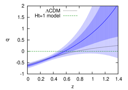
Figure 1: Deceleration parameter estimated from the Union2.1 SN data set. The dark blue line is the non-parametric smooth reconstruction based on the Gaussian process, with 68% and 95% confidence levels in lighter blue. The dashed green line presents the prediction of the $H\,t=1$ model, whereas the dotted black line is for $\Lambda$CDM.

4 Hubble rate data

We now proceed to an analysis based on observational Hubble parameter data compiled from several sources, independent of SNeIa. We combine measurements obtained with two methods: cosmic chronometers (CC), which are mainly early type and/or passively evolving galaxies, and radial baryon acoustic oscillations (BAO) from galaxy clustering in redshift surveys. Using these probes should guarantee robustness of our results: possible systematics are expected to be different in these two approaches and distinct from those in SNeIa analyses.

Based on our dataset, shortly described later in this Section, we will estimate the Hubble rate and its derivatives with respect to redshift. For the purpose of our analysis, we will normalise the Hubble parameter by its current value: $h(z)\equiv H(z)/H_{0}$. We use $H_{0}=70.4\pm 2.5\;\mathrm{km}\,\mathrm{s}^{-1}\mathrm{Mpc}^{-1}$ (Komatsu et al., 2011) throughout, although changing it to $H_{0}=74.2\pm 3.6\;\mathrm{km}\,\mathrm{s}^{-1}\mathrm{Mpc}^{-1}$ (Riess et al., 2009), preferred by MS12, would not influence our conclusions. Subsequently, we use these estimates to determine $q(z)$ and and the so-called $\mathcal{O}_{\mathrm{m}}$ diagnostic. These tests were recently applied by Seikel et al. (2012b) against the standard model and the results were consistent with $\Lambda$CDM. Here we will use the same methods and (slightly extended) data set to test the $H\,t=1$ model. Before we present the data used, let us start with the theoretical framework.

In the $H\,t=1$ model, because $a(t)=H_{0}\,t$ and owing to the general relation $a(z)=(1+z)^{-1}$ (scale factor is normalised to unity at $t_{0}$), it follows that

$$[H\,t=1]\quad h(z)=1+z\,;\quad h^{\prime}(z)=1\,;\quad h^{\prime\prime}(z)=0\;.$$ (12)

Finally, the $\mathcal{O}_{\mathrm{m}}^{(1)}$ diagnostic, first introduced by Sahni et al. (2008), is defined as

$$\mathcal{O}_{\mathrm{m}}^{(1)}(z)\equiv\frac{h^{2}(z)-1}{(1+z)^{3}-1}\;.$$ (13)

This quantity was proposed to test flat $\Lambda$CDM models because in that case it is always equal to the today’s value of the matter density parameter $\Omega_{\mathrm{m}}(t_{0})$. In the $H\,t=1$ model, $\mathcal{O}_{\mathrm{m}}^{(1)}$ is variable and depends on redshift only:

$$[H\,t=1]\qquad\mathcal{O}_{\mathrm{m}}^{(1)}(z)=\frac{2+z}{3+3z+z^{2}}\;.$$ (14)

In particular, the $H\,t=1$ model predicts that $\mathcal{O}_{\mathrm{m}}^{(1)}(t_{0})=2/3$.

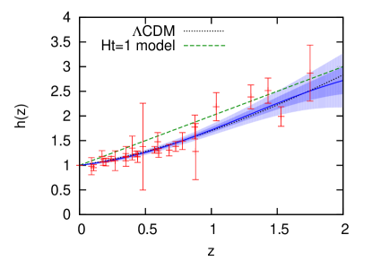
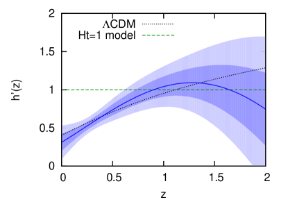
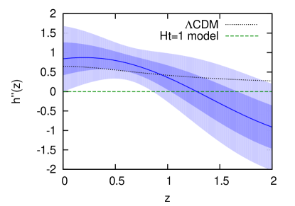
Figure 2: Top to bottom: normalised Hubble parameter, $h(z)\equiv H(z)/H_{0}$, and its two derivatives with respect to redshift. Top panel shows data points from cosmic chronometers and BAO (red crosses with errorbars). In all the panels, the dark blue lines are the non-parametric smooth reconstructions of the data, with 68% and 95% confidence levels in lighter blue; the dashed green lines present the predictions of the $H\,t=1$ model, whereas the dotted black lines are for $\Lambda$CDM.

In order to estimate the above-described quantities from observations, we will use the same data as Seikel et al. (2012b), with two data points added. The data set consists of 26 measurements of the Hubble parameter from the following sources:

• cosmic chronometers (CC): 18 data points compiled by Moresco et al. (2012b) from Simon et al. (2005), Stern et al. (2010) and Moresco et al. (2012a), spanning a redshift interval of $0.09\leq z\leq 1.75$;

• radial BAO measurements: 8 data points compiled from Gaztañaga et al. (2009), Beutler et al. (2011), Chuang & Wang (2011), Blake et al. (2012) and Reid et al. (2012), covering redshifts of $0.106\leq z\leq 0.73$.

For the reconstruction of the Hubble rate and its derivatives, we use again the Gaussian process package GaPP. Such an analysis has already been done in Seikel et al. (2012b). As we use practically the same sample (with only two BAO measurements added), our findings concerning the observed $h(z)$ etc. cannot be much different. However, unlike in Seikel et al. (2012b), here we make comparisons with the $H\,t=1$ model, which predicts particularly simple forms of the discussed functions, as given above in Equations (11), (12) and (14) [recall that $q(z)\equiv 0$ in the $H\,t=1$ model]. The comparisons are illustrated in Figures 2 and 3, presenting respectively $h(z)$, $h^{\prime}(z)$, $h^{\prime\prime}(z)$, $q(z)$ and $\mathcal{O}_{\mathrm{m}}^{(1)}(z)$. For reference, we also plot the curves for the standard flat $\Lambda$CDM model with $\Omega_{\mathrm{m}}=0.275$ (Komatsu et al., 2011).

The comparison with observational reconstructions is striking. The predictions of the $H\,t=1$ model are in clear disagreement with observations, especially at low redshifts. Very strong constraints are obtained here from the first derivative of the Hubble parameter. The $H\,t=1$ model requirement that $h^{\prime}(z)\equiv 1$ is several sigma off the data at redshifts $z<0.5$. The same conclusion can be made from the reconstruction of $q(z)$. A coasting Universe, which is predicted by the $H\,t=1$ model, is inconsistent with observations. The discrepancy is even more pronounced in the case of the $\mathcal{O}_{\mathrm{m}}^{(1)}(z)$ diagnostic (Figure 3). Here, the $H\,t=1$ model predicts much larger values than those observed, up to $z\la 1.5$. In our opinion, this single plot could be sufficient to decisively falsify the $H\,t=1$ model.

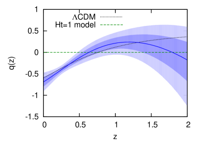
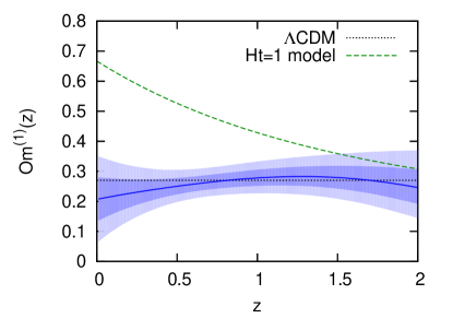
Figure 3: The deceleration parameter $q(z)$ (top) and the $\mathcal{O}_{\mathrm{m}}^{(1)}$ diagnostic of cosmic acceleration (bottom). The dark blue line is the non-parametric smooth reconstruction based on the CC+BAO data, with 68% and 95% confidence levels in lighter blue. The dashed green line presents the prediction of the $H\,t=1$ model, whereas the dotted black line is for $\Lambda$CDM.

5 Summary and conclusions

• We analysed some of the predictions of the cosmological model proposed by Melia & Shevchuk (2012), in which the scale factor growths linearly with time and the Hubble parameter is always the inverse of the age of the Universe (the ‘$H\,t=1$ model’). We started by pointing out some inconsistencies in the derivation of the model and its bizarre consequences for the nature of the Universe.

• We referred to several analyses of supernova Ia data that are all inconsistent with the $H\,t=1$ model. We presented a plot, which compares the deceleration parameter predicted by this model [$q(z)\equiv 0$] with a model-independent reconstruction of $q(z)$ obtained by applying Gaussian processes to the Union2.1 set.

• We used Hubble parameter data obtained from cosmic chronometers (18 data points with $0.09\leq z\leq 1.75$), gathered by Moresco et al. (2012b), and from baryon acoustic oscillations (8 measurements in total), combined from several sources, that spanned a redshift interval $0.106\leq z\leq 0.73$. We compared the observational data with the predictions of the $H\,t=1$ model regarding the following parameters: the Hubble parameter $H(z)$, its derivatives with respect to redshift $H^{\prime}(z)$ and $H^{\prime\prime}(z)$, as well as the $\mathcal{O}_{\mathrm{m}}(z)$ diagnostic and the deceleration parameter $q(z)$. In order to obtain derivatives of functions based on discrete data, we applied the recently developed GaPP package (Seikel et al., 2012a).

• For all these diagnostics we find severe discrepancies between the $H\,t=1$ model and observations, especially at low redshifts. The most pronounced disagreements are for the first derivative of the Hubble parameter, the $\mathcal{O}_{\mathrm{m}}$ diagnostic and the deceleration parameter. The analysed model completely fails to reproduce their observed behaviour for $z<0.5$. This strongly suggests that the cosmological model of Melia & Shevchuk (2012) is not a proper description of our Universe.

• The $R_{\mathrm{h}}=c\,t$ model proposed by Melia & Shevchuk (2012) is mathematically simple, but it does not describe the Universe we live in.

References

- Beutler et al. (2011) Beutler F. et al., 2011, MNRAS, 416, 3017
- Bilicki et al. (2011) Bilicki M., Chodorowski M., Jarrett T., Mamon G. A., 2011, ApJ, 741, 31
- Blake et al. (2012) Blake C. et al., 2012, MNRAS, 3384
- Chuang & Wang (2011) Chuang C.-H., Wang Y., 2011, arXiv e-print: [1102.2251]
- Copeland et al. (2006) Copeland E. J., Sami M., Tsujikawa S., 2006, Int.J.Mod.Ph.D, 15, 1753
- Davis et al. (2011) Davis M., Nusser A., Masters K. L., Springob C., Huchra J. P., Lemson G., 2011, MNRAS, 413, 2906
- Gaztañaga et al. (2009) Gaztañaga E., Cabré A., Hui L., 2009, MNRAS, 399, 1663
- Giostri et al. (2012) Giostri R., Vargas dos Santos M., Waga I., Reis R. R. R., Calvão M. O., Lago B. L., 2012, JCAP, 3, 27
- Guimarães et al. (2009) Guimarães A. C. C., Cunha J. V., Lima J. A. S., 2009, JCAP, 10, 10
- Guy et al. (2007) Guy J. et al., 2007, A&A, 466, 11
- Guy et al. (2005) Guy J., Astier P., Nobili S., Regnault N., Pain R., 2005, A&A, 443, 781
- Jha et al. (2007) Jha S., Riess A. G., Kirshner R. P., 2007, ApJ, 659, 122
- Komatsu et al. (2011) Komatsu E. et al., 2011, ApJS, 192, 18
- Kowalski et al. (2008) Kowalski M. et al., 2008, ApJ, 686, 749
- Kumar (2012) Kumar S., 2012, MNRAS, 422, 2532
- Lewis & van Oirschot (2012) Lewis G. F., van Oirschot P., 2012, MNRAS, 423, L26
- Lu et al. (2011) Lu J., Xu L., Liu M., 2011, Physics Letters B, 699, 246
- Melia (2012) Melia F., 2012, arXiv e-print: [1205.2713]
- Melia & Shevchuk (2012) Melia F., Shevchuk A. S. H., 2012, MNRAS, 419, 2579
- Moresco et al. (2012a) Moresco M. et al., 2012a, JCAP, 8, 6
- Moresco et al. (2012b) Moresco M., Verde L., Pozzetti L., Jimenez R., Cimatti A., 2012b, JCAP, 7, 53
- Nair et al. (2012) Nair R., Jhingan S., Jain D., 2012, JCAP, 1, 18
- Nusser & Davis (2011) Nusser A., Davis M., 2011, ApJ, 736, 93
- Peacock (1999) Peacock J. A., 1999, Cosmological Physics
- Percival et al. (2010) Percival W. J. et al., 2010, MNRAS, 401, 2148
- Perlmutter et al. (1999) Perlmutter S. et al., 1999, ApJ, 517, 565
- Reid et al. (2012) Reid B. A. et al., 2012, arXiv e-print: [1203.6641]
- Riess et al. (1998) Riess A. G. et al., 1998, AJ, 116, 1009
- Riess et al. (2009) Riess A. G. et al., 2009, ApJ, 699, 539
- Riess et al. (2004) Riess A. G. et al., 2004, ApJ, 607, 665
- Sahni et al. (2008) Sahni V., Shafieloo A., Starobinsky A. A., 2008, Physical Review D, 78, 103502
- Santos et al. (2011) Santos B., Carvalho J. C., Alcaniz J. S., 2011, Astroparticle Physics, 35, 17
- Seikel et al. (2012a) Seikel M., Clarkson C., Smith M., 2012a, JCAP, 6, 36
- Seikel & Schwarz (2009) Seikel M., Schwarz D. J., 2009, JCAP, 2, 24
- Seikel et al. (2012b) Seikel M., Yahya S., Maartens R., Clarkson C., 2012b, arXiv e-print: [1205.3431]
- Simon et al. (2005) Simon J., Verde L., Jimenez R., 2005, Physical Review D, 71, 123001
- Stern et al. (2010) Stern D., Jimenez R., Verde L., Stanford S. A., Kamionkowski M., 2010, ApJS, 188, 280
- Suzuki et al. (2012) Suzuki N. et al., 2012, ApJ, 746, 85
- van Oirschot et al. (2010) van Oirschot P., Kwan J., Lewis G. F., 2010, MNRAS, 404, 1633
- Weinberg et al. (2012) Weinberg D. H., Mortonson M. J., Eisenstein D. J., Hirata C., Riess A. G., Rozo E., 2012, arXiv e-print: [1201.2434]