Abstract

A CUSUM type test for constant correlation that goes beyond a previously suggested correlation constancy test by considering Spearman’s rho in arbitrary dimensions is proposed. Since the new test does not require the existence of any moments, the applicability on usually heavy-tailed financial data is greatly improved. The asymptotic null distribution is calculated using an invariance principle for the sequential empirical copula process. The limit distribution is free of nuisance parameters and critical values can be obtained without bootstrap techniques. A local power result and an analysis of the behavior of the test in small samples is provided.

Keywords: Copula, Mixing, Multivariate sequential rank order process, Robustness, Structural break

1 Introduction

Recently, Wied, Krämer and Dehling (2012) proposed a fluctuation test for constant correlation based on the Bravais-Pearson correlation coefficient. The test, which will be referred to as BPC test in the following, is for example useful in financial econometrics to examine changes in the correlation between asset returns over time. Longin and Solnik (1995) and Krishan et al. (2009) discuss the relevance of this question. The test complements former approaches by e.g. Galeano and Peña (2007) and Aue et al. (2009). However, one major drawback of this test is the fact that the limit distribution is derived under the condition of finite fourth moments (similar to Aue et al., 2009). This is a critical assumption because the existence of fourth moments in usually heavy-tailed financial returns is doubtful, see e.g. Grabchak and Samorodnitsky (2010), Krämer (2002) and Amaral et al. (2000).

This paper presents a fluctuation test for constant correlation based on Spearman’s rho which imposes no conditions on the existence of moments.

There are several advantages of Spearman’s rho compared to the Bravais-Pearson correlation: In many situations, e.g. if the data is non-elliptical, the Bravais-Pearson correlation may not be an appropriate measure for dependence. It is confined to measuring linear dependence, while the rank-based dependence measure Spearman’s rho quantifies monotone dependence. If the second moments do not exist, the Bravais-Pearson correlation is not even defined, while Spearman’s rho does not require any moments.

Spearman’s rho is probably the most common rank-based dependence measure in economic and social sciences, see e.g. Gaißler and Schmid (2010), who propose tests for equality of rank correlations, and the references herein. In addition, Spearman’s rho often performs better in terms of robustness than the Bravais-Pearson correlation. Embrechts et al. (2002) discuss several other pitfalls and possible problems for a risk manager who simply applies the Bravais-Pearson correlation.

Therefore, it is natural in the context of testing for changes in the dependence structure of random vectors to extend the BPC test to a test for constant Spearman’s rho. As expected from the theory of dependence measures, this test is applicable in more situations: It has a much better behavior in the presence of outliers and there are no conditions on the existence of moments. In addition, the test is applicable in arbitrary dimensions, while the BPC test is designed for bivariate random vectors. Similarly to the BPC test, the test bases on successively calculated empirical correlation coefficients in the style of Ploberger et al. (1989), Lee et al. (2003) or Galeano (2007).

The limit distribution of our test statistic is the supremum of the absolute value of a Brownian bridge. This immediately provides critical values without any bootstrap techniques. We impose a strong mixing assumption for the dependence structure. The proof relies on an invariance principle for multivariate sequential empirical processes from Bücher and Volgushev (2011).

By using the copula-based expression for Spearman’s rho from Schmid and Schmidt (2007) or Nelsen (2006), we get quite another contribution with our test, i.e. an extension of the copula constancy tests proposed by Busetti and Harvey (2011) and Krämer and van Kampen (2011). Since copula models are frequently used in financial econometrics (see e.g. Manner and Reznikova, 2011 and Giacomini et al., 2009), such tests for structural change are important in this area. However, they are restricted to the case of testing for copula constancy in one particular quantile, e.g. the $0.95$-quantile. This might be an important null hypothesis as well, but our test now (indirectly) allows for testing constancy of the whole copula by integrating over it. We therefore reject the null hypothesis of constant Spearman’s rho (which is closely connected to the null hypothesis of an overall constant copula) if the integral over it fluctuates too much over time. The problem of testing constancy of the whole copula has recently been dealt with in the literature (see Kojadinovic and Rohmer, 2012, Bücher and Ruppert, 2012, van Kampen and Wied, 2012 and Rémillard, 2010). All these approaches, however, need the computationally intensive bootstrap for approximating the limit distribution. With our approach, we need much less computational time for calculating the critical values.
The paper is organized as follows: Section 2 presents our test statistic and the asymptotic null distribution, Section 3 considers local power, Section 4 presents Monte Carlo evidence about the behavior of the test in small samples. Section 5 compares our new test with the BPC test in terms of robustness by a simulation study and an empirical application. Finally, Section 6 concludes. All proofs are in the appendix.

2 Test statistic and its asymptotic null distribution

In this section, we present the test statistic and the limit distribution of our test under the null. First, we introduce some notation: $({\bf X}_{1},\ldots,{\bf X}_{n})$ are $d$-dimensional random vectors on the probability space $(\Omega,\mathfrak{A},\mathsf{P})$ with ${\bf X}_{j}=(X_{1,j},\ldots,X_{d,j}),j=1,\ldots,n$. Regarding the dependence structure, we impose the following assumption:

1. ${\bf X}_{1},\ldots,{\bf X}_{n}$ are $\alpha$-mixing with mixing coefficients $\alpha_{j}$ satisfying

   $$\sum_{j=1}^{\infty}j^{2}\alpha_{j}^{\gamma/(4+\gamma)}<\infty$$

   for some $\gamma\in(0,2)$.

This dependence assumption is similar to the assumption made in Inoue (2001) and holds in most econometric models relevant in practice, e.g. for ARMA- and GARCH-processes under mild additional conditions, see e.g. Carrasco and Chen (2002).
The vectors ${\bf X}_{j},j=1,\ldots,n$, have joint distribution functions $F^{j}$ with

$$F^{j}({\bf x})=\mathsf{P}(X_{1,j}\leq x_{1},\ldots,X_{d,j}\leq x_{d}),{\bf x}=(x_{1},\ldots,x_{d})\in\mathbb{R}^{d},$$

and marginal distribution functions $F_{i,j}(x)=\mathsf{P}(X_{i,j}\leq x)$ for $x\in\mathbb{R}$ and $i=1,\ldots,d$ which are assumed to be continuous.
According to Sklar’s (1959) theorem, there exists a unique copula function $C_{j}:[0,1]^{d}\rightarrow[0,1]$ of ${\bf X}_{j}$ with

$$F^{j}({\bf x})=C_{j}(F_{1,j}(x_{1}),\ldots,F_{d,j}(x_{d}))$$

and

$$C_{j}({\bf u})=F_{j}(F_{1,j}^{-1}(u_{1}),\ldots,F_{d,j}^{-1}(u_{d})),{\bf u}=(u_{1},\ldots,u_{d})\in[0,1]^{d},$$

where $F^{-1}$ is the generalized inverse function, see e.g. Schmid and Schmidt (2007).

In terms of the copula, Spearman’s rho is defined as

$$\rho_{j}=h(d)\cdot\left(2^{d}\int_{[0,1]^{d}}C_{j}({\bf u})d{\bf u}-1\right)$$

with $h(d)=\frac{d+1}{2^{d}-(d+1)}$, see Schmid and Schmidt (2007) or Nelsen (2006). There are also other possibilities to define Spearman’s rho in higher dimensions (see Schmid and Schmidt, 2007 and Quessy, 2009), but we focus on this expression for ease of exposition and because this measure performs well in terms of the asymptotic relative efficiency compared with other multivariate extensions, see Quessy (2009, p. 328).
We test

$$H_{0}:\rho_{j}=\rho_{0},j=1,\ldots,n\text{ vs. }H_{1}:\exists j\in\{1,\ldots,n-1\}:\rho_{j}\neq\rho_{j+1}.$$

Let

$$\hat{F}_{i;n}(x)=\frac{1}{n}\sum_{j=1}^{n}{\bf 1}_{\{X_{i,j}\leq x\}},i=1,\ldots,d,x\in\mathbb{R},$$

$U_{i,j}=F_{i,j}(X_{i,j})$ and

$$\hat{U}_{i,j;n}:=\hat{F}_{i;n}(X_{i,j})=\frac{1}{n}\cdot\left(\text{rank of }X_{i,j}\text{ in }X_{i,1},\ldots,X_{i,n}\right),i=1,\ldots,d,j=1,\ldots,n.$$

Let $R_{j}({\bf u})={\bf 1}_{\{U_{1,j}\leq u_{1},\ldots,U_{d,j}\leq u_{d}\}}$ and $\hat{R}_{j}({\bf u})={\bf 1}_{\{\hat{U}_{1,j;n}\leq u_{1},\ldots,\hat{U}_{d,j;n}\leq u_{d}\}}$. The copula $C$ is estimated by the empirical copula, defined as

$$\hat{C}_{n}({\bf u})=\frac{1}{n}\sum_{j=1}^{n}\hat{R}_{j}({\bf u})=\frac{1}{n}\sum_{j=1}^{n}\prod_{i=1}^{d}{\bf 1}_{\{\hat{U}_{i,j;n}\leq u_{i}\}},{\bf u}=(u_{1},\ldots,u_{d})\in[0,1]^{d}.$$

The estimator based on the first $k$ observations is

$$\hat{C}_{k}({\bf u})=\frac{1}{k}\sum_{j=1}^{k}\hat{R}_{j}({\bf u})=\frac{1}{k}\sum_{j=1}^{k}\prod_{i=1}^{d}{\bf 1}_{\{\hat{U}_{i,j;n}\leq u_{i}\}},{\bf u}=(u_{1},\ldots,u_{d})\in[0,1]^{d}.$$ (1)

Note that the application of the limit theorem from Bücher and Volgushev (2011) requires that we use $\hat{U}_{i,j;n}$ and not $\hat{U}_{i,j;k}$ in (1).
The estimator for the copula immediately yields an estimator for Spearman’s rho:

$$\hat{\rho}_{k}=h(d)\cdot\left(2^{d}\int_{[0,1]^{d}}\hat{C}_{k}({\bf u})d{\bf u}-1\right)=h(d)\cdot\left(\frac{2^{d}}{k}\sum_{j=1}^{k}\prod_{i=1}^{d}(1-\hat{U}_{i,j;n})-1\right).$$

We use the test statistic $W$, defined as

$$W=\hat{D}\max_{1\leq k\leq n}\left|\frac{k}{\sqrt{n}}\left(\hat{\rho}_{k}-\hat{\rho}_{n}\right)\right|=:\hat{D}\sup_{s\in[0,1]}|P_{n}(s)|$$

with $P_{n}(s)=\frac{[ns]}{\sqrt{n}}\left(\hat{\rho}_{[ns]}-\hat{\rho}_{n}\right)$ and with a deviation estimator $\hat{D}=\frac{1}{\sqrt{\hat{D}^{\prime}}}$, where

$$\hat{D}^{\prime} =h(d)^{2}2^{2d}\left\{\frac{1}{n}\sum_{j=1}^{n}\prod_{i=1}^{d}(1-\hat{U}_{i,j;n})^{2}-\left(\frac{1}{n}\sum_{j=1}^{n}\prod_{i=1}^{d}(1-\hat{U}_{i,j;n})\right)^{2}\right.$$

$$\left.+2\left[\sum_{m=1}^{n-1}k\left(\frac{m}{\gamma_{n}}\right)\left(\sum_{j=1}^{n-m}\frac{1}{n}\prod_{i=1}^{d}(1-\hat{U}_{i,j;n})(1-\hat{U}_{i,j+m;n})-\left(\frac{1}{n}\sum_{j=1}^{n}\prod_{i=1}^{d}(1-\hat{U}_{i,j;n})\right)^{2}\right)\right]\right\}.$$

The kernel $k(\cdot)$ is selected from the class $\mathcal{K}_{2}$ of Andrews (1991), and the bandwidth $\gamma_{n}$ is chosen such that $\gamma_{n}=o(n^{\frac{1}{2}})$, see Appendix A for details. The estimator $\hat{D}$ is a scaling factor which takes serial dependence and fluctuations of the estimators for Spearman’s rho into account. The weighting factor $\frac{k}{\sqrt{n}}$ compensates for the fact that Spearman’s rho can be estimated more precisely for larger $k$.
For our main theorem, we need two additional assumptions:

1. $({\bf X}_{1},\ldots,{\bf X}_{n})$ is strictly stationary.

2. The copula $C$ and the marginal distribution functions $F_{i,j}=F_{i},i=1,\ldots,d$ are continuous.

Note that Assumption (B0) is in line with other tests for structural change, see e.g. Inoue (2001).

Theorem 1.

Under $H_{0}$ and Assumptions (A0), (B0), (B0),

$$W\rightarrow_{d}\sup_{s\in[0,1]}|B(s)|,$$

where $B(s)$ is a one-dimensional Brownian bridge.

Theorem 1 allows for constructing an asymptotic test. The main tool for the proof is an invariance principle from Bücher and Volgushev (2011) for the multivariate sequential rank order process

$$A_{n}(s,{\bf u}) :=\frac{1}{\sqrt{n}}\sum_{j=1}^{[ns]}(\hat{R}_{j}({\bf u})-\hat{C}_{n}({\bf u}))$$

$$=\frac{[ns]}{\sqrt{n}}\left(\frac{1}{[ns]}\sum_{j=1}^{[ns]}\hat{R}_{j}({\bf u})-\hat{C}_{n}({\bf u})\right),$$

which was introduced by Rüschendorf (1976). This limit condition does not require any smoothness assumption on the derivatives of the copula, see Segers (2012) for a detailed discussion of this issue.
There exists an interesting relationship between our test for constancy of Spearman’s rho and the copula constancy tests proposed by Busetti and Harvey (2011) and by Krämer and van Kampen (2011): One can show (see Appendix B) that (if $n\cdot u_{i}$ is an integer for all $i=1,\ldots,d$) our test is as a functional of the multivariate $\tau$- (or $u$-)quantics on which these copula constancy tests base. But, in fact, while the other tests examine if the copula in a particular quantile is constant, we can test for constancy of the whole copula by integrating over it. Although this is not the null hypothesis we consider, our test complements the literature on copula constancy tests.

Note that the integral of the copula (or more precisely, of the multivariate sequential rank order process) is a particular functional which has nice properties. For example, it leads to a simple limit distribution which is free of nuisance parameters, and therefore needs no bootstrap approximations. The limit distributions are more involved and/or difficult to derive with other functionals such as used in Kojadinovic and Rohmer (2012), Bücher and Ruppert (2012), van Kampen and Wied (2012) and Rémillard (2010). (van Kampen and Wied, 2012 use a slightly different definition of the multivariate sequential rank order process in that they consider the empirical quantile function $\hat{F}_{n}^{-1}$ and not the empirical distribution function $\hat{F}_{n}$.)

3 Local power

This section considers the local power of our test. Since the copula function of the random vectors under consideration changes with $n$, we now work with a triangular array $({\bf X}_{1}^{n},\ldots,{\bf X}_{n}^{n})$, but we suppress the index $n$ for ease of exposition. Let $C({\bf u})$ be a copula and let $C^{{}^{\prime}}(s,{\bf u})$ be another copula with an additional index parameter $s$. We consider local alternatives of the form

$$C_{j}({\bf u})=\left(1-\frac{\delta}{\sqrt{n}}\right)C({\bf u})+\frac{\delta}{\sqrt{n}}C^{{}^{\prime}}\left(\frac{j}{n},{\bf u}\right).$$ (2)

By choosing, say, $C^{{}^{\prime}}\left(s,{\bf u}\right)=\left[1-g(s)\right]C\left({\bf u}\right)+g(s)C^{{}^{\prime\prime}}\left({\bf u}\right)$ for some copula $C^{{}^{\prime\prime}}(\cdot)$ and some function $g(\cdot)$ bounded by $1$ we obtain the sequence of correlations

$$\rho_{j}=\left[1-\frac{\delta}{\sqrt{n}}g\left(\frac{j}{n}\right)\right]\rho_{0}+\frac{\delta}{\sqrt{n}}g\left(\frac{j}{n}\right)\rho_{A}.$$

Choosing e.g. $g(s)={\bf 1}_{\{s\geq 1/2\}}$ would lead to local alternatives in which the copula changes after the middle of the sample. A continuous function $g$ would lead to continuously changing copulas against which our test has power as well.

To deduce limit results for the sequence of local alternatives (2), we need some more assumptions:

1. The analogue of mixing condition (A0) holds for the triangular array.

2. The marginal distribution functions of $({\bf X}_{1},\ldots,{\bf X}_{n})$ do not depend on $j$ and are continuous.

3. The joint copula for the random vectors $({\bf X}_{1},\ldots,{\bf X}_{n})$ with lag $l$,

   $$C_{j,l}({\bf u_{1}},{\bf u_{2}}):=\ \mathsf{P}(X_{1,j}\leq F_{1,j}^{-1}(u_{1}^{1}),\ldots,X_{d,j}\leq F_{d,j}^{-1}(u_{1}^{d}),$$

   $$X_{1,j+l}\leq F_{1,j+l}^{-1}(u_{2}^{1}),\ldots,X_{d,j+l}\leq F_{d,j+l}^{-1}(u_{2}^{d})),$$

   is specified to

   $$C_{j,l}({\bf u_{1}},{\bf u_{2}}) =\left(1-\frac{\delta}{\sqrt{n}}\right)^{2}C_{l}({\bf u_{1}},{\bf u_{2}})+\frac{\delta^{2}}{n}C^{{}^{\prime}}_{l}\left(\frac{j}{n},\frac{j+l}{n},{\bf u_{1}},{\bf u_{2}}\right)$$

   $$+\frac{\delta}{\sqrt{n}}\left(1-\frac{\delta}{\sqrt{n}}\right)\left[C({\bf u_{1}})C^{{}^{\prime}}\left(\frac{j+l}{n},{\bf u_{2}}\right)+C({\bf u_{2}})C^{{}^{\prime}}\left(\frac{j}{n},{\bf u_{1}}\right)\right]$$

   with a constant $\delta\in(0,1]$. Here, $C_{l}(\cdot,\cdot)$ is the joint copula of some sequence of stationary random vectors $\xi_{i}$ with lag $l$, $C(\cdot)$ is the copula of $\xi_{i}$. Both $C_{l}(\cdot,cdot)$ and $C(\cdot)$ are assumed to be continuous. Analogously, $C^{{}^{\prime}}_{l}(\cdot,\cdot,\cdot,\cdot)$ is the copula of some sequence of stationary random functions $\eta_{i}(\cdot)$ with lag $l$, $C^{{}^{\prime}}(\cdot,\cdot)$ is the copula of $\eta_{i}(\cdot)$. The term $C^{\prime}(r,t)$ is continuous in $t$ for all $r$ and there is $(r,r^{\prime},t)$ such that $C^{\prime}(r,t)\neq C^{\prime}(r^{\prime},t)$.

The slightly cumbersome Assumption (C0) is similar to Assumption B in Inoue (2001) and is required for applying the limit theorem for the sequential empirical process under local alternatives and mixing conditions from Inoue (2001). Passing each element of ${\bf u_{2}}$ to $1$ yields equation (2).

With these assumptions, we get

Theorem 2.

Under Assumptions (C0) and (C0),

$$W\rightarrow_{d}\sup_{s\in[0,1]}\left|B(s)+\delta Dh(d)2^{d}\left[\int_{[0,1]^{d}}\int_{0}^{s}C^{*}\left(t,{\bf u}\right)dtd{\bf u}-s\int_{[0,1]^{d}}\int_{0}^{1}C^{*}\left(t,{\bf u}\right)dtd{\bf u}\right]\right|,$$

where $D$ is the probability limit of $\hat{D}$ under the null hypothesis.

With this theorem and Anderson’s Lemma we can deduce that the asymptotic level is always larger than or equal to $\alpha$, see Andrews (1997) or Rothe and Wied (2012).

4 Finite sample behavior

We investigate the test’s finite sample behavior and compare it to the BPC test by simulating the empirical size under the null hypothesis and the empirical power under various alternatives in different settings. Some complementary simulation results are provided in Dehling et al. (2012) who propose a bivariate test for constant Kendall’s tau.

In order to make the simulation study not too lengthy, we always use the Bartlett kernel and bandwidth $[\log(n)]$ in the deviation estimator $\hat{D}$ of our test and the deviation estimator $\tilde{D}$ of the BPC test (which is described and denoted as $\hat{D}$ in Wied et al., 2012). Moreover, we restrict ourselves to the Student copula which is one of the most common copulas for modeling financial returns according to Cherubini et al. (2004, p. 181). These choices are made in Wied et al. (2012) as well. We consider three sample sizes $n=500,1000,2000$, the significance level $\alpha=0.05$ and $50000$ repetitions in each setting. Moreover, we assume a bivariate $MA(1)$-process

$${\bf X}_{t}=\epsilon_{t}+\theta\epsilon_{t-1}\text{ with }\theta=\begin{pmatrix}\theta_{1}&0\\ 0&\theta_{2}\end{pmatrix},t=1,\ldots,n,$$

with, on the one hand, $(\theta_{1},\theta_{2})=(0,0)$ which corresponds to serial independence and, on the other hand, $(\theta_{1},\theta_{2})=(0.3,0.2)$ which corresponds to serial dependence. The $\epsilon_{t},t=0,1,\ldots,n$, are independent and identically distributed, following a bivariate $t_{\nu}$-distribution with shape matrix

$$S=\begin{pmatrix}1&q\\ q&1\end{pmatrix},\ |q|<1.$$ (3)

We consider three different degrees of freedom, $\nu=1,3,5$. In the case of $\nu=1$, we do not have finite fourth moments (even no finite first moment), which are required for the BPC test. Note that, in this case, the Bravais-Pearson correlation is not even defined. However, also in such a situation, it might be interesting to know if there is a structural change in the dependence structure. The null hypothesis is that ${\bf X}_{t}$ has constant correlation of $\rho_{0}=0.4$. Additionally, we consider seven alternatives, in which the correlation jumps after the middle of the sample from $\rho_{0}=0.4$ to $\rho_{1}=0.6,0.8,0.2,0.0,-0.2,-0.4,-0.6$, respectively. We simulate realizations $\epsilon_{0},\epsilon_{1},\ldots,\epsilon_{n/2}$ and $\epsilon_{n/2+1},\ldots,\epsilon_{n}$ with $q_{i}=\rho_{i}\sqrt{\frac{(\theta_{1}^{2}+1)(\theta_{2}^{2}+1)}{\theta_{1}\theta_{2}+1}},i=0,1$. The choice of the $q_{i}$ is due to the fact that with this, the Pearson correlation would be equal to $\rho_{0}$ resp. $\rho_{1}$ if it existed. Spearman’s rho lies then closely to these values as numerical approximations suggest.

Table 1 reports rejection frequencies for serial independence and Table 2 for serial dependence.

-Table 1 here -

-Table 2 here -

At first, we discuss the case of $\nu=1$. We see that the size of our test is kept and that the empirical power increases with the magnitude of the break and sample size $n$. It is slightly higher for increasing than for decreasing correlations. The BPC test is not applicable, because it cannot distinguish between the null and alternative hypothesis. This is partially due to the fact that the asymptotic variance of the empirical correlation coefficient is an unbounded function of the fourth moments of the population distribution and that Spearman’s correlation coefficient is invariant under monotonely increasing, componentwise transformations and hence little effected by heavy tails.

For the $t_{3}$- and $t_{5}$-distribution, the power of our copula-based test is rather low compared to the BPC test. The efficiency becomes lower when the distribution comes “closer” to the Gaussian distribution. This is not surprising as for Gaussian data, the usual empirical correlation coefficient is the maximum likelihood, i.e. the most efficient estimator of the correlation. Note however that there is compelling empirical evidence that financial returns are not Gaussian distributed.

Interestingly, the power of our test is considerably lower (up to $15$ percentage points) in the case of serial dependence as compared to independence, which is not true for the BPC test. This indicates the potential drawback that the Spearman test is more sensitive with respect to serial dependence.

While the BPC test generally detects increasing correlations better than decreasing correlations, this does not hold for the Spearman test.

Repeating the experiments from Table 2 with the $t_{2}$-distribution under serial dependence and independence yields a better behavior for the BPC test as compared to the case of $\nu=1$, but the test still does not keep its size. Our test keeps its size, and its power is generally higher than the BPC power for decreasing correlations (especially for high shifts and large sample sizes). For increasing correlations, this is true for serial independence, large sample sizes and high shifts. Detailed results are available upon request. It is an interesting task for further research to discover the area of degrees of freedom and of serial dependence in which the application of the Spearman test can be recommended.

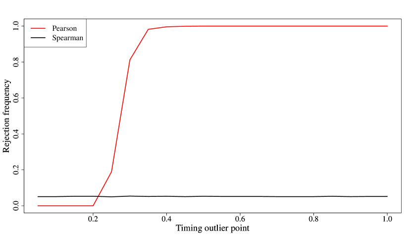
Figure 1: Empirical rejection frequencies in an outlier scenario

Next, we consider an outlier scenario by using the setup from Table 2 with the $t_{5}$-distribution, constant correlation $0.4$ and by adding one heavy outlier of size, say,
$(40,-100)$ to the sample at time $c\cdot 500,c=0.05,0.1,\ldots,1$. If the outlier comes late, the BPC test almost always rejects the null hypothesis; if it comes early, the test almost never rejects it. This is an odd behavior and makes the test unsuitable for this outlier scenario. Our new test always keeps the size, see Figure 1, whose message is basically the same in the presence of serial dependence.

-Figure 1 here -

The power of our new test becomes higher when testing for a correlation change in more than two dimensions, and when there is an equal change in every component; see Table 3 for exemplary results for the trivariate $t_{3}$-distribution under serial independence. Here, it seems that decreasing correlations are better detected. Also in the trivariate case, the power decreases in the presence of serial dependence. With more than two dimensions, a direct comparison with the BPC test is not possible because this test is restricted to two dimensions.

-Table 3 here -

5 Robustness

5.1 Simulation evidence

The two major advantages of our test compared to the BPC test proposed by Wied et al. (2012) are its applicability without any moment conditions at all (as compared to the existence of fourth moments for the BPC test) and its appealing robustness properties. The latter shall be visualized by an instructive example. Both fluctuation tests proposed here mainly derive their robustness properties from the respective properties of the underlying correlation measure. The robustness properties of Spearman’s rho, along with several other correlation estimators, are studied in detail in Croux and Dehon (2010).

Similarly to the scenario of Figure 1, we sample a path $({\bf x}_{t})_{t=1,\ldots,n}$ of length $n=500$ of the bivariate MA(1) process ${\bf X}_{t}=\epsilon_{t}+\theta\epsilon_{t-1}$, where the $\epsilon_{t}$, $t=0,\ldots,n$, are i.i.d. with a centered bivariate Gaussian distribution and covariance matrix $S$. We choose

$$\theta=\begin{pmatrix}0.3&0\\ 0&0.2\end{pmatrix}$$

and $S$ as in equation (3) with $q$ such that $\rho_{0}=0.4$.

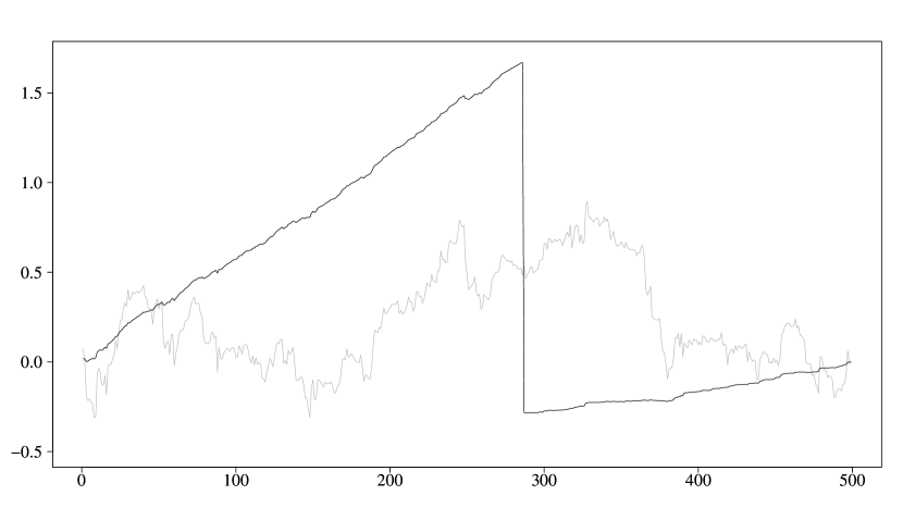
Figure 2: Process $(b_{k})_{k=1,...,500}$ computed from weakly contaminated (black) and uncontaminated (grey) sample

We add one mild outlier to the sample by setting, say, ${\bf x}_{288}$ to $(20,-50)$. We denote the resulting contaminated example by $({\bf x}_{t}^{w})_{t=1,...,n}$, where $w$ indicates weak contamination. Figure 2 visualizes the process

$$b_{k}=\tilde{D}\frac{k}{\sqrt{n}}(\hat{r}_{k}-\hat{r}_{n}),\qquad k=1,...,n,$$

where $\hat{r}_{k}$ denotes the Bravais-Pearson correlation coefficient based on ${\bf X}_{1},...,{\bf X}_{k}$, and where $\tilde{D}$ is the deviation estimator mentioned in the beginning of Section 4 that scales the process such that $(b_{[ns]})_{s\in[0,1]}$ converges to a Brownian bridge.

-Figure 2 here -

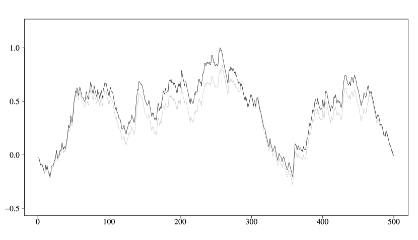
Figure 3: Process $(\psi_{k})_{k=1,...,500}$ computed from strongly contaminated (black) and uncontaminated (grey) sample

-Figure 3 here -

The BPC test statistic is then $\sup_{1\leq k\leq n}|b_{k}|$. The grey line in Figure 2 corresponds to the uncontaminated sample $({\bf x}_{t})_{t=1,...,n}$, the black line to $({\bf x}_{t}^{w})_{t=1,...,n}$. The single outlier has a dramatic effect on the Bravais-Pearson test statistic and, in this example, causes the null hypothesis to be rejected at the significance level $0.05$. While the position of the outlier influences the decision of the test (see Figure 1), it has no big influence on the basic character of the shape of the black line.

Alternatively, we create a strongly contaminated sample $({\bf x}_{t}^{s})_{t=1,...,n}$ by randomly placing $10$ outliers in the second half of the sample. Each outlier is of the form $(y_{t},-y_{t})$, where $y_{t}$ is drawn from the uniform distribution on $[-1000,-100]\cup[100,1000]$. Both, fraction and size of the outliers in $({\bf x}_{t}^{s})_{t=1,...,n}$ are about 10 times as large as in $({\bf x}_{t}^{w})_{t=1,...,n}$. Figure 3 depicts the process

$$\psi_{k}=\hat{D}\frac{k}{\sqrt{n}}(\hat{\rho}_{k}-\hat{\rho}_{n}),\qquad k=1,...,n,$$

once being computed from the uncontaminated sample (grey line) and once from the heavily corrupted sample $({\bf x}_{t}^{s})_{t=1,...,n}$ (black line). We witness a slight distortion of $(\psi_{k})_{k=1,...,n}$ as a result of the contamination, but the location of the maximizing point as well as the decision of the test are unaffected. Note that the main observations from Figure 2 and 3 basically could also be replicated under the $t_{5}$-distribution and/or serial indepedence as used in the previous section.

5.2 Empirical relevance

This subsection shows that the outlier scenario described in the previous subsection might indeed be relevant for a practitioner who analyzes structural changes in the dependence of assets. This can be exemplarily seen in the time period around the Black Monday, 19th October 1987, i.e. in the time period from the beginning of January 1985 to the end of December 1989, using daily return data from Datastream (yielding $n=1262$). Both the Dow Jones Industrial Average and the Nasdaq Composite daily returns are extremely negative at this day, and the absolute values of these returns are much higher than the other ones at this time. The next day, the Dow Jones return is positive again, while the Nasdaq return remains negative - both on a high level compared to the means and standard deviations of all days. Table 4 shows the exact values.

-Table 4 here -

These outliers are reflected in the BPC test statistic, see Figure 4, part (a), for a visualization of the process $(b_{k})_{k=1,\ldots,1262}$ and the peak around the Black Monday. On 19th October, the successively estimated correlations become very high, but fall down on the next day. Both phenomena together lead to the peak. Note that this is not exactly the same situation as in Figure 2. However, by similar simulations with two outliers as in this application, we can reproduce the peak of Figure 4, part (a), as well. Thus, the figures give two different examples of a bizarre behavior of the test statistic which are both due to the construction of the Pearson correlation coefficient.
Applying the BPC test gives a test statistic of $1.447$ ($p$-value of $0.030$) such that the null hypothesis of constant correlation is rejected at the $5\%$-level. However, the test statistic would be much lower without this peak and the null would not be rejected.
Our Spearman test statistic is not affected by this peak - see Figure 4, part (b) for a visualization of the process $(\psi_{k})_{k=1,\ldots,1262}$ - and the test statistic is equal to $0.886$ ($p$-value of $0.412$). Therefore, one should probably conclude that the dependence structure did not change seriously after the Black Monday. Similar results were obtained for other time periods around 19th October 1987 and have been confirmed in Dehling et al. (2012) who perform a related analysis.

-Figure 4 here -

6 Discussion

We propose a new test for constancy of Spearman’s rho which is much more robust against outliers than the BPC test previously suggested by Wied et al. (2012).

Indirectly, our test also allows for testing if the whole copula of multivariate random vectors is constant, and thus it extends formerly suggested pointwise copula constancy tests. It is an interesting task for further research to compare the performance of our test with the performance of constancy tests for the whole copula, based on other functionals of the multivariate sequential rank order process, such as proposed in Kojadinovic and Rohmer (2012), Bücher and Ruppert (2012), van Kampen and Wied (2012) and Rémillard (2010), especially in higher dimensions. Some limited evidence for the bivariate case (Spearman and maximum functional) can be found in van Kampen and Wied (2012) and van Kampen (2012). In general, it is not obvious how to compare both tests as one needs to specify a bandwidth for the Spearman test and a block length for the maximum test. However, there is evidence that the Spearman test is typically (but not always) outperformed by the maximum test in terms of power. The Spearman test is computationally less intensive as no bootstrap approximations are required.

Another worthwile research approach would be an extension of the considered dependence structure to functionals of iid- or even of mixing processes in order to enlarge the class of models in which our test can operate.

Appendix A Appendix section

Proof of Theorem 1
Denote with $l^{\infty}(\mathbb{R}^{k})$ the function space of all bounded functions from $\mathbb{R}^{k}$ to $\mathbb{R}$.

Consider first $P_{n}(s)$:

$$P_{n}(s) =\frac{[ns]}{\sqrt{n}}\left(h(d)\cdot\left(2^{d}\int_{[0,1]^{d}}\hat{C}_{[ns]}({\bf u})d{\bf u}-1\right)-h(d)\cdot\left(2^{d}\int_{[0,1]^{d}}\hat{C}_{n}({\bf u})d{\bf u}-1\right)\right)$$

$$=\frac{[ns]}{\sqrt{n}}\cdot h(d)\cdot 2^{d}\int_{[0,1]^{d}}\left(\frac{1}{[ns]}\sum_{j=1}^{[ns]}\hat{R}_{j}({\bf u})-\frac{1}{n}\sum_{j=1}^{n}\hat{R}_{j}({\bf u})\right)d{\bf u}$$

$$=h(d)\cdot 2^{d}\int_{[0,1]^{d}}A_{n}(s,{\bf u})d{\bf u}$$

with

$$A_{n}(s,{\bf u})=\frac{[ns]}{\sqrt{n}}\left(\frac{1}{[ns]}\sum_{j=1}^{[ns]}\hat{R}_{j}({\bf u})-\frac{1}{n}\sum_{j=1}^{n}\hat{R}_{j}({\bf u})\right).$$ (4)

With an invariance principle for

$$\frac{1}{\sqrt{n}}\sum_{j=1}^{[ns]}(R_{j}({\bf u})-C({\bf u})),$$ (5)

which is presented in Theorem 2.1 in Inoue (2001) (setting $\delta$ from Inoue, 2001 to $0$ and defining $x_{ni}$ from Inoue, 2001 as $(F_{i}(X_{i,j}))_{1\leq i\leq d}$), Condition 3.1 in Bücher and Volgushev (2011) is satisfied with $G_{n}^{*}(s,{\bf u}):=\frac{1}{n}\sum_{j=1}^{[ns]}R_{j}({\bf u})$ and $C^{*}(s,{\bf u}):=sC({\bf u})$ which lies in the space $\mathbb{D}_{\Psi}$ defined in Bücher and Volgushev (2011). So we obtain with Corollary 3.3.a in Bücher and Volgushev (2011)

$$A_{n}(\cdot,\cdot)\rightarrow_{d}A_{0}(\cdot,\cdot)\text{ in }l^{\infty}(\mathbb{R}^{d+1})$$

with

$$A_{0}(s,{\bf u})=V_{0}(s,{\bf u})-sV_{0}(1,{\bf u}).$$

$V_{0}(s,{\bf u})$ is a $\mathsf{P}$-almost surely continuous, centered Gaussian process with covariance function

$$K_{0}((s_{1},{\bf u_{1}}),(s_{2},{\bf u_{2}})):=\mathsf{Cov}(V_{0}(s_{1},{\bf u_{1}}),V_{0}(s_{2},{\bf u_{2}}))=(s_{1}\wedge s_{2})K^{\prime}({\bf u_{1}},{\bf u_{2}}),$$

where

$$K^{\prime}({\bf u_{1}},{\bf u_{2}}) =C({\bf u_{1}}\wedge{\bf u_{2}})-C({\bf u_{1}})C({\bf u_{2}})$$

$$+\sum_{m=2}^{\infty}\left(\mathsf{E}({\bf 1}_{\{X_{1,1}\leq F_{1}^{-1}(u_{1}^{1});\ldots;X_{d,1}\leq F_{d}^{-1}(u_{1}^{d})\}}{\bf 1}_{\{X_{1,m}\leq F_{1}^{-1}(u_{2}^{1});\ldots;X_{d,m}\leq F_{d}^{-1}(u_{2}^{d})\}})\right.$$

$$\left.-\mathsf{E}({\bf 1}_{\{X_{1,1}\leq F_{1}^{-1}(u_{1}^{1});\ldots;X_{d,1}\leq F_{d}^{-1}(u_{1}^{d})\}})\cdot\mathsf{E}({\bf 1}_{\{X_{1,m}\leq F_{1}^{-1}(u_{2}^{1});\ldots;X_{d,m}\leq F_{d}^{-1}(u_{2}^{d})\}})\right)$$

$$+\sum_{m=2}^{\infty}\left(\mathsf{E}({\bf 1}_{\{X_{1,1}\leq F_{1}^{-1}(u_{2}^{1});\ldots;X_{d,1}\leq F_{d}^{-1}(u_{2}^{d})\}}{\bf 1}_{\{X_{1,m}\leq F_{1}^{-1}(u_{1}^{1});\ldots;X_{d,m}\leq F_{d}^{-1}(u_{1}^{d})\}})\right.$$

$$\left.-\mathsf{E}({\bf 1}_{\{X_{1,1}\leq F_{1}^{-1}(u_{2}^{1});\ldots;X_{d,1}\leq F_{d}^{-1}(u_{2}^{d})\}})\cdot\mathsf{E}({\bf 1}_{\{X_{1,m}\leq F_{1}^{-1}(u_{1}^{1});\ldots;X_{d,m}\leq F_{d}^{-1}(u_{1}^{d})\}})\right).$$

This covariance function is the limit of the covariance function of

$$V_{n}(s,{\bf u}) =\frac{1}{\sqrt{n}}\sum_{j=1}^{[ns]}(R_{j}({\bf u})-C({\bf u})),$$

i.e.

$$K_{0}((s_{1},{\bf u_{1}}),(s_{2},{\bf u_{2}}))=\lim_{n\rightarrow\infty}\mathsf{Cov}(V_{n}(s_{1},{\bf u_{1}}),V_{n}(s_{2},{\bf u_{2}})),$$

see Inoue (2001). Now, with the continuous mapping theorem,

$$P_{n}(\cdot)\rightarrow_{d}P_{0}(\cdot)\text{ in }l^{\infty}(\mathbb{R}),$$

where

$$P_{0}(s)=h(d)2^{d}\int_{[0,1]^{d}}A_{0}(s,{\bf u})d{\bf u}$$

is a $\mathsf{P}$-almost surely continuous, centered Gaussian process. With Fubini’s theorem, the covariance function is

$$\mathsf{Cov}(P_{0}(s_{1}),P_{0}(s_{2}))$$

$$=h(d)^{2}2^{2d}\int_{[0,1]^{d}}\int_{[0,1]^{d}}\mathsf{Cov}(V_{0}(s_{1},{\bf u_{1}})-s_{1}V_{0}(1,{\bf u_{1}}),V_{0}(s_{2},{\bf u_{2}})-s_{2}V_{0}(1,{\bf u_{2}}))d{\bf u_{1}}d{\bf u_{2}}$$

$$=h(d)^{2}2^{2d}(s_{1}\wedge s_{2}-s_{1}s_{2}-s_{1}s_{2}+s_{1}s_{2})\int_{[0,1]^{d}}\int_{[0,1]^{d}}\mathsf{Cov}(V_{0}(1,{\bf u_{1}}),V_{0}(1,{\bf u_{2}}))d{\bf u_{1}}d{\bf u_{2}}$$

$$=(s_{1}\wedge s_{2}-s_{1}s_{2})D^{\prime}$$

with

$$D^{\prime} =h(d)^{2}2^{2d}\int_{[0,1]^{d}}\int_{[0,1]^{d}}K^{\prime}({\bf u_{1}},{\bf u_{2}})d{\bf u_{1}}d{\bf u_{2}}$$

$$=h(d)^{2}2^{2d}\left\{\mathsf{E}\left(\prod_{i=1}^{d}(1-U_{i,j})^{2}\right)-\left[\mathsf{E}\left(\prod_{i=1}^{d}(1-U_{i,j})\right)\right]^{2}\right.$$

$$\left.+2\left[\sum_{m=1}^{\infty}\mathsf{E}\left(\prod_{i=1}^{d}(1-U_{i,j})(1-U_{i,j+m})\right)-\left(\mathsf{E}\left(\prod_{i=1}^{d}(1-U_{i,j})\right)\right)^{2}\right]\right\}$$

$$=h(d)2^{2d}\left[\mathsf{Var}\left(\prod_{i=1}^{d}(1-U_{i,j})\right)+2\sum_{m=1}^{\infty}\mathsf{Cov}\left(\prod_{i=1}^{d}(1-U_{i,j}),\prod_{i=1}^{d}(1-U_{i,j+m})\right)\right].$$

This holds because, again with Fubini,

$$\int_{[0,1]^{d}}\int_{[0,1]^{d}}C({\bf u_{1}}\wedge{\bf u_{2}})d{\bf u_{1}}d{\bf u_{2}}$$

$$=\int_{[0,1]^{d}}\int_{[0,1]^{d}}\mathsf{E}({\bf 1}_{\{X_{1,j}\leq F_{1}^{-1}(u_{1}^{1});\ldots;X_{d,j}\leq F_{d}^{-1}(u_{1}^{d})\}}{\bf 1}_{\{X_{1,j}\leq F_{1}^{-1}(u_{2}^{1});\ldots;X_{d,j}\leq F_{d}^{-1}(u_{2}^{d})\}})d{\bf u_{1}}d{\bf u_{2}}$$

$$=\mathsf{E}\left(\int_{[0,1]^{d}}\int_{[0,1]^{d}}{\bf 1}_{\{X_{1,j}\leq F_{1}^{-1}(u_{1}^{1});\ldots;X_{d,j}\leq F_{d}^{-1}(u_{1}^{d})\}}{\bf 1}_{\{X_{1,j}\leq F_{1}^{-1}(u_{2}^{1});\ldots;X_{d,j}\leq F_{d}^{-1}(u_{2}^{d})\}}d{\bf u_{1}}d{\bf u_{2}}\right)$$

$$=\mathsf{E}\left(\int_{[0,1]^{d}}\int_{[0,1]^{d}}{\bf 1}_{\{U_{1,j}\leq u_{1}^{1};\ldots;U_{d,j}\leq u_{1}^{d}\}}{\bf 1}_{\{U_{1,j}\leq u_{2}^{1};\ldots;U_{d,j}\leq u_{2}^{d}\}}d{\bf u_{1}}d{\bf u_{2}}\right)$$

$$=\mathsf{E}\left(\prod_{i=1}^{d}(1-U_{i,j})\prod_{i=1}^{d}(1-U_{i,j})\right).$$

The other summands of $K^{\prime}({\bf u_{1}},{\bf u_{2}})$ are integrated analoguesly.
We get a consistent estimator for $D^{\prime}$ from de Jong and Davidson (2000),

$$\tilde{D}^{\prime} =h(d)^{2}2^{2d}\left\{\frac{1}{n}\sum_{j=1}^{n}\prod_{i=1}^{d}(1-U_{i,j})^{2}-\left(\frac{1}{n}\sum_{j=1}^{n}\prod_{i=1}^{d}(1-U_{i,j})\right)^{2}\right.$$

$$\left.+2\left[\sum_{m=1}^{n-1}k\left(\frac{m}{\gamma_{n}}\right)\left(\sum_{j=1}^{n-m}\frac{1}{n}\prod_{i=1}^{d}(1-U_{i,j})(1-U_{i,j+m})-\left(\frac{1}{n}\sum_{j=1}^{n}\prod_{i=1}^{d}(1-U_{i,j})\right)^{2}\right)\right]\right\},$$

with a kernel $k$ that is contained in the class $\mathcal{K}_{2}$ of Andrews (1991) which guarantees positive semi-definiteness of $\tilde{D}^{\prime}$. Next, we show that $\hat{D}^{\prime}-\tilde{D}^{\prime}\rightarrow_{p}0$. By the invariance principle (5) (this time applied on the components of ${\bf X}_{j}$) we get a Glivenko-Cantelli-like theorem (in probability) with rate $n^{-\frac{1}{2}}$ for the marginal empirical distribution functions, that means,

$$B_{n}:=\max_{i=1,\ldots,d}\sup_{j\in\mathbb{N}}|\hat{U}_{i,j;n}-U_{i,j}|=O_{\mathsf{P}}\left(n^{-\frac{1}{2}}\right).$$

Since $0\leq U_{i,j},\hat{U}_{i,j;n}\leq 1$, we obtain

$$\left|\prod_{i=1}^{d}(1-\hat{U}_{i,j;n})(1-\hat{U}_{i,j+m;n})-\prod_{i=1}^{d}(1-U_{i,j})(1-U_{i,j+m})\right|\leq 2dB_{n}.$$

Thus we get

$$|\hat{D}^{\prime}-\tilde{D}^{\prime}|\leq C\sum_{m=1}^{n-1}k\left(\frac{m}{\gamma_{n}}\right)B_{n}=O_{\mathsf{P}}\left(\gamma_{n}n^{-\frac{1}{2}}\right)=o_{\mathsf{P}}(1),$$

as $\gamma_{n}=o(n^{\frac{1}{2}})$, compare the argument in Andrews (1991, p. 852). Therefore $\hat{D}^{\prime}$ is a consistent estimator of $D^{\prime}$.
The theorem follows then with the continuous mapping theorem, because the process

$$P^{*}_{0}(s):=\frac{1}{\sqrt{D^{\prime}}}P_{0}(s)$$

is a $\mathsf{P}$-almost surely continuous, centered Gaussian process with the same covariance function as the Brownian bridge, i.e.

$$\mathsf{Cov}(P^{*}_{0}(s_{1}),P^{*}_{0}(s_{2}))=s_{1}\wedge s_{2}-s_{1}s_{2}.$$

Since a Gaussian process is uniquely determined by the first two moments, the limit process is in fact a Brownian bridge. $\blacksquare$

Proof of Theorem 2
The proof is basically similar to the proof of Theorem 1. We consider $A_{n}(s,{\bf u})$ from (4) and use a minor modification of Corollary 3.3.a in Bücher and Volgushev (2011). Condition 3.1 is modified in that sense that we formulate the condition for triangular arrays. The invariance principle from Theorem 2.1 in Inoue (2001) (defining again $x_{ni}$ from Inoue, 2001 as $(F_{i}(X_{i,j}))_{1\leq i\leq d}$ with the stationarity of the marginal distribution functions) yields that

$$\frac{1}{\sqrt{n}}\sum_{j=1}^{[ns]}(R_{j}({\bf u})-C_{j}({\bf u}))$$ (6)

converges in distribution to the process $V_{0}(s,{\bf u})$ such that

$$\frac{1}{\sqrt{n}}\sum_{j=1}^{[ns]}(R_{j}({\bf u})-C({\bf u})) =\frac{1}{\sqrt{n}}\sum_{j=1}^{[ns]}(R_{j}({\bf u})-C_{j}({\bf u}))+\frac{1}{\sqrt{n}}\sum_{j=1}^{[ns]}(C_{j}({\bf u})-C({\bf u}))$$ (7)

$$=\frac{1}{\sqrt{n}}\sum_{j=1}^{[ns]}(R_{j}({\bf u})-C_{j}({\bf u}))+\frac{\delta}{n}\sum_{j=1}^{[ns]}\left(C^{{}^{\prime}}\left(\frac{j}{n},{\bf u}\right)-C({\bf u})\right)$$ (8)

converges in distribution to the process $V_{0}(s,{\bf u})+\delta\int_{0}^{s}C^{{}^{\prime}}\left(t,{\bf u}\right)dt-\delta sC({\bf u})$. This process fulfills Condition 3.1 in Bücher and Volgushev (2011) with $G_{n}^{*}(s,{\bf u})=\frac{1}{n}\sum_{j=1}^{[ns]}R_{j}({\bf u})$ and $C^{*}(s,{\bf u})=sC({\bf u})$ which lies in the space $\mathbb{D}_{\Psi}$ defined in Bücher and Volgushev (2011). Thus the proof of Corollary 3.3.a goes through in the same way as in the stationarity case. Thus, $A_{n}(s,{\bf u})$ converges to

$$A_{0}(s,{\bf u})+\delta\left[\int_{0}^{s}C^{{}^{\prime}}\left(t,{\bf u}\right)dt-s\int_{0}^{1}C^{{}^{\prime}}\left(t,{\bf u}\right)dt\right].$$

In addition, the probability limit of $\hat{D}$ under the sequence of local alternatives is the quantity $D$ from the proof of Theorem 1, i.e. the probability limit of $\hat{D}$ under the null hypothesis. This holds because

$$\lim_{n\rightarrow\infty}\mathsf{Cov}(V_{n}(s_{1},{\bf u_{1}}),V_{n}(s_{2},{\bf u_{2}}))$$

is the same under the null hypothesis as well as under the sequence of local alternatives. Thus, the theorem is proved. $\blacksquare$

Appendix B Connection to copula constancy tests

Let $\hat{F}_{i,n}^{-1}(u_{i}),0<u_{i}<1,i=1,\ldots,d,$ denote the empirical quantile function and consider the case that $n\cdot u_{i}$ is an integer for all $i=1,\ldots,d$. Write

$$A_{n}(s,u) = \frac{[ns]}{\sqrt{n}}\left(\frac{1}{[ns]}\sum_{j=1}^{[ns]}\hat{R}_{j}(u)-\frac{1}{n}\sum_{j=1}^{n}\hat{R}_{j}(u)\right)$$

$$= -\frac{[ns]}{\sqrt{n}}\left(\frac{1}{[ns]}\sum_{j=1}^{[ns]}\left(\hat{C}_{n}(u)-\hat{R}_{j}(u)\right)\right)+\frac{[ns]}{\sqrt{n}}\left(\frac{1}{n}\sum_{j=1}^{n}\left(\hat{C}_{n}(u)-\hat{R}_{j}(u)\right)\right)$$

$$= -\frac{1}{\sqrt{n}}\sum_{j=1}^{[ns]}\left(\hat{C}_{n}(u)-\hat{R}_{j}(u)\right)+\frac{1}{\sqrt{n}}\sum_{k=1}^{[ns]}\left(\frac{1}{n}\sum_{j=1}^{n}\left(\hat{C}_{n}(u)-\hat{R}_{j}(u)\right)\right)$$

$$= -\frac{1}{\sqrt{n}}\sum_{j=1}^{[ns]}\left[\left(\hat{C}_{n}(u)-\hat{R}_{j}(u)\right)-\frac{1}{n}\sum_{m=1}^{n}\left(\hat{C}_{n}(u)-\hat{R}_{m}(u)\right)\right]$$

$$= -\frac{1}{\sqrt{n}}\sum_{j=1}^{[ns]}\left[\hat{C}_{n}(u)-{\bf 1}_{\{X_{1j}\leq\hat{F}_{1,n}^{-1}(u_{1}),\ldots,X_{dj}\leq\hat{F}_{d,n}^{-1}(u_{d})\}}\right],$$

where the last step uses that $1/n\sum_{m=1}^{n}\hat{R}_{m}(u)=\hat{C}_{n}(u)$ and

$$\hat{R}_{j}(u) := {\bf 1}_{\{\hat{U}_{1j;n}\leq u_{1},\ldots,\hat{U}_{dj;n}\leq u_{d}\}}$$

$$= {\bf 1}_{\{\hat{F}_{1,n}^{-1}(\hat{U}_{1j;n})\leq\hat{F}_{1,n}^{-1}(u_{1}),\ldots,\hat{F}_{d,n}^{-1}(\hat{U}_{dj;n})\leq\hat{F}_{d,n}^{-1}(u_{d})\}}$$

$$= {\bf 1}_{\{X_{1j}\leq\hat{F}_{1,n}^{-1}(u_{1}),\ldots,X_{dj}\leq\hat{F}_{d,n}^{-1}(u_{d})\}}.$$

Note that $\hat{C}_{n}(u)-{\bf 1}_{\{X_{1j}\leq\hat{F}_{1,n}^{-1}(u_{1}),\ldots,X_{dj}\leq\hat{F}_{d,n}^{-1}(u_{d})\}}$ are the bivariate $\tau$- or $u$-quantics in Busetti and Harvey (2011) if $d=2$. Hence, our test bases on similar quantities.

Acknowledgements: Financial support by Deutsche Forschungsgemeinschaft (SFB 823, Statistik nichtlinearer dynamischer Prozesse, projects A1 and C3) and Ruhr Graduate School in Economics is gratefully acknowledged. We are grateful to helpful comments from the Editor, the Associate Editor and the referees.

(a) Process $(b_{k})_{k=1,\ldots,1262}$

(b) Process $(\psi_{k})_{k=1,\ldots,1262}$

Figure 4: Processes $(b_{k})_{k=1,\ldots,1262}$ and $(\psi_{k})_{k=1,\ldots,1262}$ for the Dow Jones and Nasdaq Index

Table 1: Empirical power in different settings with serial independence, $\rho_{0}=0.4$, results of the Pearson-test in brackets

$n$	Values of $\rho_{1}$
	$0.4$	$0.6$	$0.8$	$0.2$	$0$	$-0.2$	$-0.4$	$-0.6$
a) bivariate $t_{1}$ distribution
$500$	$0.045$	$0.081$	$0.205$	$0.079$	$0.199$	$0.418$	$0.702$	$0.917$
	$(0.478)$	$(0.507)$	$(0.550)$	$(0.474)$	$(0.476)$	$(0.490)$	$(0.513)$	$(0.533)$
$1000$	$0.046$	$0.121$	$0.383$	$0.120$	$0.370$	$0.730$	$0.953$	$0.998$
	$(0.477)$	$(0.505)$	$(0.553)$	$(0.469)$	$(0.479)$	$(0.490)$	$(0.511)$	$(0.539)$
$2000$	$0.048$	$0.205$	$0.662$	$0.204$	$0.656$	$0.960$	$1.000$	$1.000$
	$(0.477)$	$(0.500)$	$(0.550)$	$(0.471)$	$(0.475)$	$(0.489)$	$(0.514)$	$(0.538)$
b) bivariate $t_{3}$ distribution
$500$	$0.045$	$0.085$	$0.217$	$0.088$	$0.230$	$0.495$	$0.786$	$0.958$
	$(0.050)$	$(0.260)$	$(0.725)$	$(0.125)$	$(0.412)$	$(0.699)$	$(0.843)$	$(0.907)$
$1000$	$0.045$	$0.129$	$0.404$	$0.134$	$0.426$	$0.804$	$0.978$	$1.000$
	$(0.040)$	$(0.352)$	$(0.845)$	$(0.195)$	$(0.602)$	$(0.831)$	$(0.916)$	$(0.950)$
$2000$	$0.048$	$0.222$	$0.699$	$0.230$	$0.732$	$0.983$	$1.000$	$1.000$
	$(0.035)$	$(0.479)$	$(0.910)$	$(0.310)$	$(0.756)$	$(0.906)$	$(0.951)$	$(0.968)$
c) bivariate $t_{5}$ distribution
$500$	$0.047$	$0.085$	$0.215$	$0.089$	$0.240$	$0.515$	$0.804$	$0.966$
	$(0.038)$	$(0.435)$	$(0.958)$	$(0.261)$	$(0.778)$	$(0.962)$	$(0.990)$	$(0.995)$
$1000$	$0.047$	$0.129$	$0.404$	$0.136$	$0.446$	$0.824$	$0.984$	$1.000$
	$(0.038)$	$(0.693)$	$(0.992)$	$(0.506)$	$(0.955)$	$(0.993)$	$(0.998)$	$(0.999)$
$2000$	$0.048$	$0.226$	$0.698$	$0.237$	$0.753$	$0.987$	$1.000$	$1.000$
	$(0.037)$	$(0.913)$	$(0.998)$	$(0.806)$	$(0.992)$	$(0.998)$	$(0.999)$	$(1.000)$

Table 2: Empirical power in different settings with serial dependence, $\rho_{0}=0.4$, results of the Pearson-test in brackets

$n$	Values of $\rho_{1}$
	$0.4$	$0.6$	$0.8$	$0.2$	$0$	$-0.2$	$-0.4$	$-0.6$
a) bivariate $t_{1}$ distribution
$500$	$0.053$	$0.077$	$0.165$	$0.078$	$0.157$	$0.313$	$0.545$	$0.790$
	$(0.481)$	$(0.513)$	$(0.563)$	$(0.478)$	$(0.479)$	$(0.495)$	$(0.519)$	$(0.539)$
$1000$	$0.056$	$0.108$	$0.294$	$0.107$	$0.282$	$0.573$	$0.850$	$0.980$
	$(0.480)$	$(0.510)$	$(0.565)$	$(0.472)$	$(0.483)$	$(0.494)$	$(0.517)$	$(0.546)$
$2000$	$0.056$	$0.165$	$0.513$	$0.164$	$0.504$	$0.861$	$0.990$	$1.000$
	$(0.480)$	$(0.506)$	$(0.561)$	$(0.473)$	$(0.478)$	$(0.492)$	$(0.518)$	$(0.544)$
b) bivariate $t_{3}$ distribution
$500$	$0.051$	$0.082$	$0.183$	$0.084$	$0.191$	$0.401$	$0.671$	$0.895$
	$(0.054)$	$(0.286)$	$(0.760)$	$(0.136)$	$(0.438)$	$(0.722)$	$(0.857)$	$(0.915)$
$1000$	$0.053$	$0.119$	$0.327$	$0.122$	$0.347$	$0.693$	$0.933$	$0.996$
	$(0.044)$	$(0.385)$	$(0.868)$	$(0.213)$	$(0.630)$	$(0.848)$	$(0.923)$	$(0.954)$
$2000$	$0.055$	$0.188$	$0.573$	$0.193$	$0.610$	$0.941$	$0.999$	$1.000$
	$(0.037)$	$(0.520)$	$(0.924)$	$(0.337)$	$(0.777)$	$(0.915)$	$(0.955)$	$(0.970)$
c) bivariate $t_{5}$ distribution
$500$	$0.053$	$0.083$	$0.182$	$0.087$	$0.200$	$0.423$	$0.696$	$0.911$
	$(0.042)$	$(0.465)$	$(0.968)$	$(0.273)$	$(0.792)$	$(0.967)$	$(0.991)$	$(0.995)$
$1000$	$0.054$	$0.118$	$0.331$	$0.124$	$0.366$	$0.719$	$0.947$	$0.998$
	$(0.041)$	$(0.725)$	$(0.994)$	$(0.529)$	$(0.961)$	$(0.994)$	$(0.998)$	$(0.999)$
$2000$	$0.055$	$0.192$	$0.581$	$0.199$	$0.640$	$0.953$	$0.999$	$1.000$
	$(0.040)$	$(0.929)$	$(0.998)$	$(0.822)$	$(0.993)$	$(0.998)$	$(0.999)$	$(1.000)$

Table 3: Empirical power in different settings for the trivariate $t_{3}$-distribution with serial independence, $\rho_{0}=0.4$ (for $\rho_{1}=-0.6$, the shape matrix would not be positively definite)

$n$	Values of $\rho_{1}$
	$0.4$	$0.6$	$0.8$	$0.2$	$0$	$-0.2$	$-0.4$
$500$	$0.042$	$0.169$	$0.534$	$0.195$	$0.695$	$0.988$	$1.000$
$1000$	$0.043$	$0.311$	$0.850$	$0.368$	$0.955$	$1.000$	$1.000$
$2000$	$0.046$	$0.570$	$0.992$	$0.660$	$1.000$	$1.000$	$1.000$

Table 4: Dow Jones and Nasdaq Returns around the Black Monday and empirical moments of the whole time span

Day	16.10.	19.10.	20.10.	21.10.	22.10.	$\hat{\mu}$	$\hat{\sigma}$
Dow Jones	$-0.047$	$-0.256$	$0.057$	$0.097$	$-0.039$	$0.001$	$0.013$
Nasdaq	$-0.039$	$-0.120$	$-0.094$	$0.071$	$-0.046$	$0.001$	$0.009$

References

- Amaral et al. (2000) Amaral, L., V. Plerou, P. Gopikrishan, M. Meyer, and H. Stanley (2000): “The distribution of returns of stock prices,” International Journal of Theoretical and Applied Finance, 3(3), 365–369.
- Andrews (1991) Andrews, D. (1991): “Heteroskedasticity and autocorrelation consistent covariance matrix estimation,” Econometrica, 59(3), 817–858.
- Andrews (1997) ——— (1997): “A conditional Kolmogorov test,” Econometrica, 65, 1097–1128.
- Aue et al. (2009) Aue, A., S. Hörmann, L. Horvath, and M. Reimherr (2009): “Break detection in the covariance structure of multivariate time series models,” Annals of Statistics, 37(6B), 4046–4087.
- Bücher and Ruppert (2012) Bücher, A. and M. Ruppert (2012): “Consistent testing for a constant copula under strong mixing based on the tapered block multiplier technique,” Journal of Multivariate Analysis, forthcoming.
- Bücher and Volgushev (2011) Bücher, A. and S. Volgushev (2011): “Empirical and sequential empirical copula processes under serial dependence,” preprint, arXiv: 1111.2778.
- Busetti and Harvey (2011) Busetti, F. and A. Harvey (2011): “When is a copula constant? A test for changing relationships,” Journal of Financial Econometrics, 9(1), 106–131.
- Carrasco and Chen (2002) Carrasco, M. and X. Chen (2002): “Mixing and moment properties of various GARCH and stochastic volatility models,” Econometric Theory, 18, 17–39.
- Cherubini et al. (2004) Cherubini, U., E. Luciano, and W. Vecchiato (2004): Copula methods in finance, Wiley, Chichester.
- Croux and Dehon (2010) Croux, C. and C. Dehon (2010): “Influence functions of the Spearman and Kendall Correlation measures,” Statistical Methods and Applications, 19(4), 497–515.
- de Jong and Davidson (2000) de Jong, R. and J. Davidson (2000): “Consistency of kernel estimators of heteroscedastic and autocorrelated covariance matrices,” Econometrica, 68(2), 407–424.
- Dehling et al. (2012) Dehling, H., D. Vogel, M. Wendler, and D. Wied (2012): “An efficient and robust test for change-points in correlation,” working paper (arXiv:1203.4871v2).
- Embrechts et al. (2002) Embrechts, P., A. McNeil, and D. Straumann (2002): “Correlation and dependence in risk management: Properties and pitfalls,” in Risk management: Value at Risk and beyond, ed. by M. Dempster, Cambridge University Press, Cambridge, 176–223.
- Gaißler and Schmid (2010) Gaißler, S. and F. Schmid (2010): “On testing equality of pairwise rank correlations in a multivariate random vector,” Journal of Multivariate Analysis, 101, 2598–2615.
- Galeano (2007) Galeano, P. (2007): “The use of cumulative sums for detection of changepoints in the rate parameter of a Poisson Process,” Computational Statistics and Data Analysis, 51(12), 6151–6165.
- Galeano, P. and D. Peña (2007) Galeano, P. and D. Peña (2007): “Covariance changes detection in multivariate time series,” Journal of Statistical Planning and Inference, 137(1), 194–211.
- Giacomini et al. (2009) Giacomini, E., W. Härdle, and V. Spokoiny (2009): “Inhomogeneous Dependence Modeling with Time-Varying Copulae,” Journal of Business and Economic Statistics, 27(2), 224–234.
- Grabchak and Samorodnitsky (2010) Grabchak, M. and G. Samorodnitsky (2010): “Do financial returns have finite or infinite variance? A paradox and an explanation,” Quantitative Finance, 10(8), 883–893.
- Inoue (2001) Inoue, A. (2001): “Testing for distributional change in time series,” Econometric Theory, 17, 156–187.
- Kojadinovic and Rohmer (2012) Kojadinovic, I. and T. Rohmer (2012): “Asymptotics and multiplier bootstrap of the sequential empirical copula process with applications to change-point detection,” working paper (arXiv:1206.2557.v1).
- Krishan et al. (2009) Krishan, C., R. Petkova, and P. Ritchken (2009): “Correlation risk,” Journal of Empirical Finance, 16, 353–367.
- Krämer (2002) Krämer, W. (2002): “Statistische Besonderheiten von Finanzzeitreihen,” Jahrbücher für Nationalökonomie und Statistik, 222, 210–229.
- Krämer and van Kampen (2011) Krämer, W. and M. van Kampen (2011): “A simple nonparametric test for structural change in joint tail probabilities,” Economics Letters, 110, 245–247.
- Lee et al. (2003) Lee, S., J. Ha, O. Na, and S. Na (2003): “The CUSUM test for parameter change in time series models,” Scandinavian Journal of Statistics, 30(4), 781–796.
- Longin and Solnik (1995) Longin, F. and B. Solnik (1995): “Is the correlation in international equity returns constant: 1960-1990?” International Money and Finance, 14(1), 3–26.
- Manner and Reznikova (2011) Manner, H. and O. Reznikova (2011): “A survey on time-varying copulas: Specification, simulations and application,” Econometric Reviews, 31(6), 654–687.
- Nelsen (2006) Nelsen, R. (2006): An introduction to copulas, Springer, 2 ed.
- Ploberger et al. (1989) Ploberger, W., W. Krämer, and K. Kontrus (1989): “A new test for structural stability in the linear regression model,” Journal of Econometrics, 40, 307–318.
- Quessy (2009) Quessy, J.-F. (2009): “Theoretical efficiency comparisons of independence tests based on multivariate versions of Spearman’s rho,” Metrika, 70, 315–338.
- Rémillard (2010) Rémillard, B. (2010): “Goodness-of-fit tests for copulas of multivariate time series,” SSRN working paper, online: http://dx.doi.org/10.2139/ssrn.1729982.
- Rothe and Wied (2012) Rothe, C. and D. Wied (2012): “Misspecification testing in a class of conditional distributional models,” Journal of the American Statistical Association, forthcoming.
- Rüschendorf (1976) Rüschendorf, L. (1976): “Asymptotic distributions of multivariate rank order statistics,” Annals of Statistics, 4(5), 912–923.
- Schmid and Schmidt (2007) Schmid, F. and R. Schmidt (2007): “Multivariate extensions of Spearman’s rho and related statistics,” Statistics and Probability letters, 77, 407–416.
- Segers (2012) Segers, J. (2012): “Asymptotics of empirical copula processes under nonrestrictive smoothness assumptions,” Bernoulli, 18(3), 764–782.
- Sklar (1959) Sklar, A. (1959): “Fonctions de répartition à dimensions et leurs marges,” Publications de l’Institut de Statistique de L’Université de Paris, 8, 229–231.
- van Kampen (2012) van Kampen, M. (2012): Copula constancy tests, Dissertation, TU Dortmund.
- van Kampen and Wied (2012) van Kampen, M. and D. Wied (2012): “A nonparametric constancy test for copulas under mixing conditions,” preprint (TU Dortmund).
- Wied et al. (2012) Wied, D., W. Krämer, and H. Dehling (2012): “Testing for a change in correlation at an unknown point in time using an extended functional delta method,” Econometric Theory, 58(3), 570–589.