Criticality governed by the stable renormalization fixed point
of the Ising model in the hierarchical small-world network

Abstract

We study the Ising model in a hierarchical small-world network by renormalization group analysis, and find a phase transition between an ordered phase and a critical phase, which is driven by the coupling strength of the shortcut edges. Unlike ordinary phase transitions, which are related to unstable renormalization fixed points (FPs), the singularity in the ordered phase of the present model is governed by the FP that coincides with the stable FP of the ordered phase. The weak stability of the FP yields peculiar criticalities including logarithmic behavior. On the other hand, the critical phase is related to a nontrivial FP, which depends on the coupling strength and is continuously connected to the ordered FP at the transition point. We show that this continuity indicates the existence of a finite correlation-length-like quantity inside the critical phase, which diverges upon approaching the transition point.

Recently, various physical phenomena in non-Euclidean graphs have been studied especially in the context of complex networks, and their properties have been found to be beyond the scope of the conventional theory for Euclidean graphs Dorogovtsev et al. (2008). Of particular interest are systems regarded as infinite dimensional in the sense that the equidistant surface $S_{r}$ of radius $r$ grows exponentially as $S_{r}\propto e^{y_{d}r}$ with a positive constant $y_{d}$, which is faster than any power function $r^{d-1}$ as in $d$-dimensional Euclidean graphs. Typical examples are trees and hyperbolic lattices Shima and Sakaniwa (2006). Remarkably, such infinite-dimensional systems often exhibit the critical phases in which the (nonlinear) susceptibility diverges Hinczewski and Berker (2006); Berker et al. (2009); Nogawa and Hasegawa (2009a). Although the critical phase is also observed in some Euclidean systems, e.g., the quasi-long-range ordered phase in the two-dimensional XY model Berezinskii (1972); Kosterlitz and Thouless (1973), the critical phases in infinite dimensional systems are considered to be due to rather geometrical effects. Indeed, the exponential growth of a graph admits the divergence of the susceptibility $\chi$, which is calculated by the integral of the two-point correlation function , even with finite correlation length $\hat{\xi}$ Nogawa and Hasegawa (2009b); for $\hat{\xi}>1/y_{d}$

$$\chi\propto\int_{0}^{\ln N/y_{d}}drS_{r}e^{-r/\hat{\xi}}\propto N^{\psi},\quad\psi\equiv 1-1/y_{d}\hat{\xi}$$ (1)

diverges in the thermodynamic limit $N\to\infty$. Here we set the upper bound $\ln N/y_{d}$ to ensure $\chi\propto N$ for $\hat{\xi}=\infty$. A critical phase, if it exists, lies between a disordered phase with $\hat{\xi}<1/y_{d}$ and an ordered phase with $\hat{\xi}=\infty$. Such a phase with a fractal exponent $0<\psi<1$ is actually observed in the percolation transitions in enhanced trees Nogawa and Hasegawa (2009a), hyperbolic lattices Baek et al. (2009), hierarchical graphs Hasegawa et al. (2010); Boettcher et al. (2012), and growing random networks Hasegawa and Nemoto (2010).

(a)                            (b)

Figure 1: (a) Hierarchical small-world network with eight nodes. The periodic boundary condition is imposed on the horizontal direction. (b) One-step decimation of the central spin in the partial sum of partition function. This is an inverse procedure to grow the graph in (a).

The property of the phase transitions between a critical phase and an ordered phase is an interesting issue. Quite recently, some models in the simple hierarchical network shown in Fig. 1(a) were investigated to examine these transitions. This network is very useful because rigorous real-space renormalization is possible for various models in the simplest way. Furthermore various types of phase transition are observed depending on the model used, e.g., a discontinuous transition of the bond percolation model Boettcher et al. (2012), equivalent to the 1-state Potts model Kasteleyn and Fortuin (1969); Fortuin and Kasteleyn (1972), and continuous transitions with a power-law singularity (PLS) or an essential singularity (ES) for the $q$-state Potts model with $q\geq 3$ Nogawa et al. (2012). These are observed in other graphs Krapivsky and Derrida (2004); Hinczewski and Berker (2006); Boettcher et al. (2009); Berker et al. (2009); Nogawa and Hasegawa (2009a). Thus this hierarchical network is a good stage to investigate what determines the type of phase transitions in a systematic way. In particular the 2-state Potts model, equivalent to the Ising model, stands between $q=1$ and $q=3$, and has special importance to understand how the transition class changes.

In this Rapid Communication, we study the phase transition of the 2-state Potts model in the network mentioned above by renormalization group (RG) analysis, which reveals a new class of phase transition governed by the stable fixed point. Furthermore the singularity for $q=2$ is found to be special due to the marginal bifurcation of the RG fixed point (FP) between pitchfork type for $q<2$ and saddle-node type for $q>2$.

We consider the 2-state Potts model in the hierarchical small-world network shown in Fig. 1(a). This consists of one-dimensional backbone edges (BBEs) and nested shortcut edges (SCEs). The spin variable $\sigma$, taking a value 0 or 1, is put on every node of the network. The dimensionless energy function is written as

$$-\frac{E}{k_{\mathrm{B}}T}=\!\!\sum_{\mathrm{\langle i,j\rangle\in BBE}}\!\!K\delta_{\sigma_{i}\sigma_{j}}+\!\!\sum_{\mathrm{\langle i,j\rangle\in SCE}}\!\!J\delta_{\sigma_{i}\sigma_{j}}+\sum_{i}H\delta_{\sigma_{i}0},$$ (2)

where $K$ and $J$ are the coupling constants on BBEs and SSEs, respectively, and $H(>0)$ denotes the external magnetic field coupled with the state 0.

Let us consider the partial sum of the partition function $Z=\prod_{i}\sum_{\sigma_{i}}e^{-E/k_{B}T}$ over the states of spins in the youngest generation having two neighbors [see Fig. 1(b)]. This is rigorously equivalent to replacing the parameters as

$$C_{n+1}e^{K_{n+1}\delta_{\sigma_{1}\sigma_{2}}+(H_{n+1}/2)(\delta_{\sigma_{1}0}+\delta_{\sigma_{2}0})}$$

$$=C_{n}^{2}e^{(H_{n}/2)(\delta_{\sigma_{1}0}+\delta_{\sigma_{2}0})}\sum_{\sigma}e^{(K_{n}+J)(\delta_{\sigma\sigma_{1}}+\delta_{\sigma\sigma_{2}})+H_{n}\delta_{\sigma 0}},$$ (3)

with the recursion relations:

$$g_{n+1} \!\!=\!\! g_{n}+2^{-(n+1)}\!\left[K_{n}+J-A^{(1)}_{n}/2+A^{(2)}_{n}/2+A^{(3)}_{n}\right],$$

$$K_{n+1} \!\!=\!\! -(K_{n}+J)+A^{(1)}_{n}/2+A^{(2)}_{n}/2-A^{(3)}_{n},$$ (4)

$$H_{n+1} \!\!=\!\! H_{n}+A^{(1)}_{n}-A^{(2)}_{n},$$ (5)

where $g_{n}=2^{-n}\ln C_{n}$, $e^{A^{(1)}_{n}}=e^{2(K_{n}+J)+H_{n}}+1$, $e^{A^{(2)}_{n}}=e^{2(K_{n}+J)}+e^{H_{n}}$, and $e^{A^{(3)}_{n}}=e^{H_{n}}+1$.

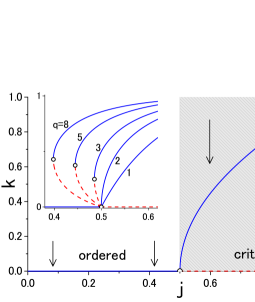
Figure 2: (color online) Phase diagram in the $j$ vs $k$ plain. The shaded region indicates the critical phase. The (blue) solid line and (red) dashed line denote stable and unstable fixed lines, respectively. The arrows indicate the RG flow of $k$. The inset shows the fixed lines for $q$=1, 2, 3, 5, and 8.

For $H=0$, the recursion relation is rewritten as

$$k_{n+1}-k_{n}=-\frac{k_{n}\left[j^{2}k_{n}^{2}-(2j-1)\right]}{1+j^{2}k_{n}^{2}},$$ (6)

where we put $k_{n}=e^{-K_{n}}$ and $j=e^{-J}$. The FP is given by $k_{n+1}=k_{n}=k^{*}$, which is solved as

$$k^{*}=0,\pm\sqrt{2t/(1+t)},\quad t\equiv 2j-1.$$ (7)

There is a pitchfork bifurcation point (PF BP) at $(j,k)=(1/2,0)$; the stable FP is $k^{*}=0$ for $j\leq 1/2$ and $k^{*}=\sqrt{2t/(1+t)}$ for $j>1/2$ (see Fig. 2). The region where the flow goes to the nontrivial fixed line is regarded as a critical phase because each FP on the line represents a self-similar structure like an ordinary critical point. It is noteworthy that in this renormalization procedure the couplings on the SCEs remain the same while the ones on the BBEs are updated. The SCE couplings $0<J\ll 1$ prevent $K_{n}$ from converging to zero, and therefore the critical phase appears instead of a disordered phase. A similar mechanism is observed in the RG analysis of the Ising models exhibiting the critical phases, e.g., in graphs: the decorated (2,2)-flower Hinczewski and Berker (2006) and the Hanoi network with average degree 5 (HN5) Boettcher and Brunson (2011).

When $j$ increases with $k$ fixed, a transition from the ordered phase to the critical phase occurs at $j=j_{c}=1/2$, irrespectively of the value of $k$. Remarkably, the FP at $j_{c}$ corresponds to $K=\infty(k=0)$ as well as in the ordered phase $j<j_{c}$ and is stable, so that the critical behavior is quite unlike the conventional one governed by unstable FP (US FP). This yields a curious singularity, as shown below.

Equation (6) is approximated by a differential equation:

$$\frac{ds_{n}}{dn}=-\frac{2s_{n}(s_{n}+|t|)}{1+s_{n}},\quad s_{n}\equiv k_{n}^{2}j^{2}.$$ (8)

This is solved as $e^{-2n|t|}=\frac{s_{n}}{s_{0}}\left(\frac{s_{0}+|t|}{s_{n}+|t|}\right)^{1-|t|}$ leading to

$$s_{n}\approx\frac{|t|}{e^{2n|t|}-1}=\left\{\begin{array}[]{ccc}1/2n&\mathrm{for}&n|t|\ll 1\\ |t|e^{-2n|t|}&\mathrm{for}&n|t|\gg 1\end{array}\right.$$ (11)

for $|t|\ll s_{0}$. Since $s_{n}$ goes to zero for $n\rightarrow\infty$, it is (and thus $K$ is) an irrelevant parameter.

In the lowest order of $H_{n}$, Eq. (11) is still valid as a solution of Eq. (4). On the other hand, Eq. (5) is rewritten as

$$H_{n+1}=H_{n}+\ln\frac{e^{2(K_{n}+J)+H_{n}}+1}{e^{2(K_{n}+J)}+e^{H_{n}}}=\frac{2H_{n}}{1+s_{n}}+O(H_{n}^{2}).$$ (12)

Note that we leave $s_{n}$ in the first term; the cross term of $s_{n}$ and $H_{n}$ remains and thus this is beyond the linear stability analysis. By putting $H_{n}=2^{n}e^{-x_{n}}$, we obtain

$$x_{n}\approx\sum_{\ell=n_{0}}^{n-1}s_{\ell}\approx\int_{n_{0}}^{n}\frac{|t|d\ell}{e^{2\ell|t|}-1}=\frac{1}{2}\ln\frac{1-e^{-2n|t|}}{1-e^{-2n_{0}|t|}},$$ (13)

where we substitute Eq. (11) into the summation and approximate it by the integral. Here we give the lower bound of summation $n_{0}$ to avoid the divergence of $s_{\ell}$ at $\ell=0$. Finally we obtain

$$H_{n}=He^{ny_{d}}u_{n}$$

$$u_{n}\approx\sqrt{\frac{|t|}{1-e^{-2n|t|}}}\propto\left\{\begin{array}[]{ccc}n^{-1/2}&\mathrm{for}&n|t|\ll 1\\ |t|^{1/2}&\mathrm{for}&n|t|\gg 1\end{array}\right.\!,$$ (16)

where we use $y_{d}=\ln 2$. Note that the factor $u_{n}$ does not appear in the linear-order treatment for $s_{n}$ and $H_{n}$.

The RG evolution Eq. (16) leads to a scale-invariant formula of the free energy as

$$g(H,N^{-1})=e^{-ny_{d}}g(Hu_{n}e^{ny_{d}},N^{-1}e^{ny_{d}})$$ (17)

for $n\gg 1$. Here $t$ is not included explicitly in the arguments of $g$ because it is (and thus $J$ is) not a scaling field but just an external parameter. The irrelevant scaling field $s_{n}$ is also omitted. However the effect of $s_{n}$ is indirectly included in $H_{n}$ as in Eq. (12) and gives the $t$ dependence as in Eq. (16). The first and second order derivatives of $g$ with $H$ are written as

$$g_{H}(H,N^{-1}) = u_{n}g_{H}(Hu_{n}e^{ny_{d}},N^{-1}e^{ny_{d}}),$$ (18)

$$g_{H^{2}}(H,N^{-1}) = u_{n}^{2}e^{ny_{d}}g_{H^{2}}(Hu_{n}e^{ny_{d}},N^{-1}e^{ny_{d}}),$$ (19)

respectively. In the following, we show the behaviors of the magnetization $m=g_{H}$ and the susceptibility $\chi=g_{H^{2}}$ in three asymptotic regimes: (i) $t<0$, $H=0$ and $N=\infty$, (ii) $t=0$, $H>0$ and $N=\infty$, and (iii) $t=0$, $H=0$ and $N<\infty$.

(i) For $t<0$, $H=0$ and $N=e^{ny_{d}}\rightarrow\infty$, we obtain

$$m = |t|^{1/2}g_{H}(0,1)\propto|t|^{1/2},$$ (20)

$$\chi = N|t|g_{H^{2}}(0,1)\propto N|t|,$$ (21)

with $u_{n}\rightarrow|t|^{1/2}$. The magnetization shows the PLS as if it were an ordinary second order transition. Within the linear analysis $u_{n}=1$, $m$ does not vanish at $t=0$, and the transition would look discontinuous. Surprisingly, $\chi$ diverges in the whole ordered phase, meaning the coexistence of a divergent fluctuation and a nonzero order parameter. Such coexistence may be realized by spatial segregation into the fluctuating region and the ordered region around the root node, the left most node in Fig. 1(a).

(ii) For $t\rightarrow 0$ and $N=e^{ny_{d}}$, $u_{n}\rightarrow n^{-1/2}$, Eqs. (18) and (19) become

$$g_{H}(H,N^{-1}) = n^{-1/2}g_{H}(Hn^{-1/2}e^{ny_{d}},1),$$ (22)

$$g_{H^{2}}(H,N^{-1}) = n^{-1}e^{ny_{d}}g_{H^{2}}(Hn^{-1/2}e^{ny_{d}},1).$$ (23)

We set $n$ so as to satisfy $Hn^{-1/2}e^{ny_{d}}=1$, which is approximately solved as $e^{ny_{d}}\approx\ln(H^{-1})/y_{d}H$. By substituting this into Eqs. (22) and (23), we obtain

$$m \approx \sqrt{\frac{y_{d}}{\ln(H^{-1})}}g_{H}(1,1)\propto\left[\ln(H^{-1})\right]^{-1/2},$$ (24)

$$\chi \approx \frac{y_{d}}{\ln H^{-1}}\frac{\ln{H^{-1}}}{y_{d}H}g_{H^{2}}(1,1)\propto\frac{1}{H}.$$ (25)

(iii) For $t=0$ and $H=0$, Eqs. (22) and (23) become

$$m = \sqrt{\frac{y_{d}}{\ln N}}g_{H}(0,1)\propto\left(\ln N\right)^{-1/2},$$ (26)

$$\chi = \frac{N}{\ln N}g_{H^{2}}(0,1)\propto\frac{N}{\ln N}.$$ (27)

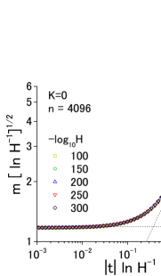
Figure 3: (color online) Scaling plot of the magnetization in the ordered phase. Data with $m<0.20$ are used.

On the crossover between the two limits, Eqs. (20) and (24), we expect a one-parameter scaling formula for $N=\infty$ such as

$$m=t^{1/2}\tilde{m}(t\ln H^{-1})=\left[\ln(H^{-1})\right]^{-1/2}\tilde{\tilde{m}}(t\ln H^{-1}),$$ (28)

which is confirmed in Fig. 3. We numerically calculate $m$ by integrating the recursion equations of $g_{n}$, $K_{n}$, $H_{n}$, and their derivatives.

Next, we investigate the property of the critical phase ($t>0$). By considering the linear stability of Eqs. (4) and (5) at the points on the fixed line, we obtain $\tilde{K}_{n+1}=e^{ny_{K}(t)}\tilde{K}_{n}$ and $H_{n+1}=e^{ny_{H}(t)}H_{n}$ where $\tilde{K}_{n}\equiv K_{n}-K^{*}(t)$, $y_{K}(t)=\ln\frac{1-t}{1+t},\quad\mathrm{and}\quad y_{H}(t)=\ln\frac{2}{1+t}.$ These lead to $\tilde{K}_{n}\propto e^{ny_{K}}$ and $H_{n}\propto e^{ny_{H}}$. While $y_{K}(t)$ is negative and therefore $\tilde{K}$ is irrelevant in the critical phase, $y_{H}(t)$ is positive and approaches $y_{d}=\ln 2$ from below as $t\rightarrow 0_{+}$.

The free energy in the critical phase satisfies

$$g(H,N^{-1})=e^{-ny_{d}}g(He^{ny_{H}(t)},N^{-1}e^{ny_{d}}).$$

Again we omit the irrelevant parameters $\tilde{K}$ and $t$ from the arguments, but $t$-dependence is included in $y_{H}$. The $\ell$-th order derivative of $g$ is written as

$$g_{H^{\ell}}(H,N^{-1})=e^{n(\ell y_{H}(t)-y_{d})}g_{H^{\ell}}(He^{ny_{H}(t)},N^{-1}e^{ny_{d}}).$$

Since $y_{H}(t)<y_{d}$, the first order derivative, i.e., the magnetization, is zero for $H=0$ and $N=e^{ny_{d}}\rightarrow\infty$ in the critical phase. The susceptibility for $H=0$ and $N=e^{ny_{d}}$ is

$$\chi=N^{\psi(t)}g_{H^{2}}(0,1)\propto N^{\psi(t)}$$ (29)

$$\psi(t)=2\frac{y_{H}(t)}{y_{d}}-1=1-\frac{2}{\ln 2}\ln(1+t).$$ (30)

For $1/2<j<1/\sqrt{2}$, $\psi$ varies from 1 to 0 as shown in Fig. 4. In this region, $\chi$ diverges in the thermodynamic limit. For $j>1/\sqrt{2}$, $\chi$ is finite but higher order derivatives, i.e., nonlinear susceptibilities, diverge; the $\ell$th order derivative of the free energy with $H$ diverges in the region where $\ell y_{H}(t)>y_{d}$.

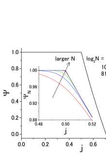
Figure 4: (color online) The fractal exponent is plotted with respect to the BBE coupling constant. The inset enlarges the finite size behavior $\psi_{N}$ around $j=j_{c}=1/2$.

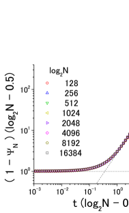
Figure 5: (color online) Scaling plot of the fractal exponent $\psi_{N}$ in the critical phase. Data with $\psi_{N}>0.60$ are used.

As noted in Eq. (1), $\psi$ is related to the correlation length $\hat{\xi}$, and the fact that $\psi$ approaches 1 from below means the divergence of $\hat{\xi}$. Here we consider the finite size effect of this singularity. The inset of the Fig. 4 shows the fractal exponent for size $N$ defined as $\psi_{N}\equiv\log_{2}[\chi(N)/\chi(N/2)]$. If we assume a power-law divergence of $\hat{\xi}$, a finite size scaling formula,

$$\hat{\xi}^{-1} \equiv 1-\psi_{N}=t^{\nu}F(t^{\nu}[\ln N]^{\mu})$$ (33)

$$= \left\{\begin{array}[]{ccc}t^{\nu}&\mathrm{for}&t^{\nu}[\ln N]^{\mu}\gg 1\\ \left[\ln N\right]^{-\mu}&\mathrm{for}&t^{\nu}[\ln N]^{\mu}\ll 1\end{array}\right.,$$

is expected for $H=0$. If $\ln N$ is a proper cutoff length, $\mu$ should be unity. Equations (30) and (27) lead to $1-\psi_{N}\propto t$ and $1-\psi_{N}\propto[\ln N]^{-1}$, respectively. Thus $\nu=1$ and $\mu=1$. We confirm the scaling behavior Eq. (33) in Fig. 5.

We have investigated the 2-state Potts (Ising) model in the simple hierarchical network with the real-space RG method. The phase transition between the ordered and critical phases is governed by the PF BP at $K=\infty$ independently of the bare value of $K$. The singular behavior of the present model is summarized in Table 1, where we also show the Potts model with $q=1$ Boettcher et al. (2012) and $q\geq 3$ Nogawa et al. (2012). See also the inset of Fig. 2 for the fixed lines for various $q$ systems.

Boettcher et al. studied the bond percolation model, i.e., the 1-state Potts model, in the same graph without backbone ($K=0$) Boettcher et al. (2012), and found a PF bifurcation of the RG FP similar to the present model ($q=2$). They also calculate the maximum cluster size $\langle s_{\mathrm{max}}\rangle$, which is a quantity corresponding to unconnected susceptibility $\tilde{\chi}\equiv\chi+Nm^{2}$ because both quantities are defined as a summation of the two-point correlation. For $q=1$, however, discontinuity of $\langle s_{\mathrm{max}}\rangle/N$ is observed at the transition point. This is in contrast to the fact that $\tilde{\chi}/N\propto t$ for $q=2$. By taking the analytic continuation of the recursion relation, corresponding to Eq. (6), for $q\geq 3$ in Ref. Nogawa et al. (2012), we obtain the PF BP $(j,k)=(1/2,0)$ for $q\leq 2$ and the recursion relation at $j=1/2$: $k_{n+1}-k_{n}=-\frac{2-q}{4}k^{2}-\frac{q-1}{4}k^{3}+O(k^{4})$. Thus the FP of $q=2$ is marginal and has weaker stability. This is presumably the origin of the continuity of the transition.

For $q\geq 3$, the saddle-node (SN) bifurcation of the FP is observed Nogawa et al. (2012). Consequently, two kinds of singularity appear depending on $k=e^{-K}$: ES corresponding to SN BP for $k\geq k_{\mathrm{SN}}$ and PLS corresponding to USFP for $k<k_{\mathrm{SN}}$. The SN BP $(j_{\mathrm{SN}},k_{\mathrm{SN}})$ approaches the PF BP $(1/2,0)$ as $q\rightarrow 2$. While the PLS and ES for $q\geq 3$ are governed by USFP and marginally unstable SN BP, respectively, the phase transition for $q\leq 2$ is governed by the stable FP. Thus the generalized scaling theory in Ref. Nogawa et al. (2012) assuming instability of a FP cannot be applied to the latter. We emphasize that the stability or instability of the FP of the transition point is the most fundamental criterion of phase transitions.

$q$	FP	$m$	$\chi$	$\hat{\xi}\equiv 1/(1-\psi)$
$1$	PF BP	–	$N|t|^{0}$, –	$t^{-2},\ [\ln N]^{2}$
$2$	PF BP	$\sqrt{|t|},\ [\ln H^{-1}]^{-1/2}$	$N|t|,\ H^{-1}$	$t^{-1},\ln N$
$\geq 3$	SN BP	$e^{-|t|^{-1/2}},\ H^{1/\delta}$	$e^{|t|^{-1/2}},\ H^{1/\delta-1}$	$t^{0}$
$\geq 3$	USFP	$|t|^{\beta},H^{1/\delta}$	$|t|^{-\gamma},\ H^{1/\delta-1}$	$t^{0}$

Table 1: Summary of singularities. We show the singular formula of $m$ and $\chi$ in the ordered phase $t<0$ and of $\hat{\xi}$ in the critical phase $t>0$. A discontinuous change is noted as $t^{0}$. The fact that $\hat{\xi}\propto[\ln N]^{2}$ for $q=1$ is our preliminary result of a Monte Carlo simulation.

References

Dorogovtsev et al. (2008)
S. N. Dorogovtsev,
A. V. Goltsev,
and J. F. F.
Mendes, Rev. Mod. Phys.
80, 1275 (2008).
Shima and Sakaniwa (2006)
H. Shima and
Y. Sakaniwa,
J. Stat. Mech. p. 08017
(2006).
Hinczewski and Berker (2006)
M. Hinczewski and
A. N. Berker,
Phys. Rev. E 73,
066126 (2006).
Berker et al. (2009)
A. N. Berker,
M. Hinczewski,
and R. R. Netz,
Phys. Rev. E 80,
041118 (2009).
Nogawa and
Hasegawa (2009a)
T. Nogawa and
T. Hasegawa,
J. Phys. A: Math. Theor. 42,
145001 (2009a).
Berezinskii (1972)
V. L. Berezinskii,
Sov. Phys. JETP 34,
610 (1972).
Kosterlitz and Thouless (1973)
J. M. Kosterlitz
and D. J.
Thouless, J. Phys. C
6, 1181 (1973).
Nogawa and
Hasegawa (2009b)
T. Nogawa and
T. Hasegawa,
J. Phys. A: Math. Theor. 42,
478002 (2009b).
Baek et al. (2009)
S. K. Baek,
P. Minnhagen,
and B. J. Kim,
Phys. Rev. E 79,
011124 (2009).
Hasegawa et al. (2010)
T. Hasegawa,
M. Sato, and
K. Nemoto,
Phy. Rev. E 82,
046101 (2010).
Boettcher et al. (2012)
S. Boettcher,
V. Singh, and
R. M. Ziff,
Nature Communications 3,
787 (2012).
Hasegawa and Nemoto (2010)
T. Hasegawa and
K. Nemoto,
Phy. Rev. E 81,
051105 (2010).
Kasteleyn and Fortuin (1969)
P. W. Kasteleyn
and C. M.
Fortuin, J. Phys. Soc. Jap.
26, 11 (1969).
Fortuin and Kasteleyn (1972)
C. M. Fortuin and
P. W. Kasteleyn,
Physica 57,
536 (1972).
Nogawa et al. (2012)
T. Nogawa,
T. Hasegawa, and
K. Nemoto,
Phys. Rev. Lett. 108,
255703 (2012).
Krapivsky and Derrida (2004)
P. L. Krapivsky
and B. Derrida,
Physica A 340,
714 (2004).
Boettcher et al. (2009)
S. Boettcher,
J. L. Cook, and
R. M. Ziff,
Phys. Rev. E 80,
041115 (2009).
Boettcher and Brunson (2011)
S. Boettcher and
C. T. Brunson,
Phys. Rev. E 83,
021103 (2011).
Bauer et al. (2005)
M. Bauer,
S. Coulomb, and
S. N. Dorogovtsev,
Phys. Rev. Lett. 94,
200602 (2005).