Abstract

We study the toroidal dipole moment of the lightest neutralino in the constrained Minimal Supersymmetric Standard Model. The toroidal dipole moment is the only electromagnetic property of the neutralino. Since the neutralino is the LSP in many versions of the MSSM and therefore a candidate for dark matter, its characterization through its electromagnetic properties is important both for particle physics and for cosmology. We perform a scan in the parameter space of the cMSSM and find that the toroidal dipole moment is different from zero, albeit very small, in all the parameter space, and reaches a value around $10^{-3}$ GeV^-2 in a particular region of the parameter space, well below experimental bounds.

1 Introduction

One of the best motivated extensions of the Standard Model (SM) is the Minimal Supersymmetric Standard Model (MSSM), since, besides giving a solution to the hierarchy problem, provides us with a good candidate for cold dark matter (CDM), namely, the lightest neutralino.

There are currently several experiments under way, and more planned for the future for direct and indirect detection of dark matter (DM) (for recent reviews on dark matter direction see [1, 2]). If detected, it will be necessary to discriminate between different candidates. To this end, it will be important to characterize as much as possible the different candidates. The neutralino is at present one of the best candidates for DM, and its electroweak properties can give us some insight into its nature. Because it is neutral, these properties appear only radiatively.

Recently, there has been intense work on the electroweak properties of dark matter since they might be relevant in the calculation of DM decays and annihilations [3, 4, 5, 6, 7, 8, 9, 10, 11, 12, 13, 14, 15], which have consequences in astrophysical processes [16, 17] and therefore are important in indirect astrophysical searches for DM, as in the calculation of the annihilation cross section of the DM itself.

One of the least studied electromagnetic properties of a particle is the Toroidal Dipole Moment (TDM), which is directly related to the anapole moment. The anapole moment corresponds to a $T$ invariant interaction, which is $C$ and $P$ non-invariant [18]. It does not have a simple classical analogue, thus the toroidal dipole moment was introduced as a more convenient description of $T$ even, $C$ and $P$ odd, interactions [19, 20, 21, 22]. The electromagnetic vertex of a particle can thus be expressed in a multipole parametrization, including the toroidal moments (see for instance [23]), which provides a one to one correspondence between the form factors and the multipole moments.

Pospelov and ter Veldhuis have obtained an upper limit for the anapole moment of WIMPS [24], using results from the DAMA and CDMS experiments [25, 26]. In case the neutralino is the main component of dark matter, its anapole moment should comply with this limit.

In this paper we calculate the TDM of the neutralino within the constrained Minimal Supersymmetric Standard Model. We do a scan in the five parameter space of the cMSSM, and compare the results with the above mentioned experimental limit. The article is organised as follows: in section II we present a very brief summary of some aspects of the constrained MSSM (cMSSM) relevant to our calculation. In section III we review the general form for the electromagnetic vertex of a particle, and in particular for a Majorana particle, as the neutralino. We introduce the anapole moment and its relation to the toroidal dipole moment. In section IV we explain the methodology used to calculate the TMD of the neutralino in the cMSSM and we evaluate it for different values of the parameters. Section V presents the results obtained and our conclusions.

2 The MSSM and the neutralino as candidate for dark matter

The cold dark matter density is known to be [27]

$$\Omega_{DM}h^{2}\sim 0.112~{},$$ (1)

where $h$ is the Hubble constant in units of $100$ km sec^-1 Mpc^-1. The thermally averaged effective cross section times the relative speed of the dark matter particle, needed to get this relic density is [28, 29, 30]

$$<\sigma v>\propto g^{4}_{weak}/16\pi^{2}m_{x}^{2}$$ (2)

consistent with the assumption of a weakly interacting dark matter particle (WIMP) with mass between $10~{}$GeV - $(few)$ TeV.

The minimal supersymmetric extension of the Standard Model (MSSM) provides us with one of the best WIMP candidates for dark matter, namely the lighest neutralino (for reviews on SUSY see for instance [31, 32]). The MSSM requires two complex Higgs electroweak doublets to give mass to the up and down type quarks and to avoid chiral anomalies. After electroweak symmetry breaking five physical Higgs states remain: two neutral CP invariant $\left(h^{0},H^{0}\right)$, two charged CP invariant $\left(H^{+},H^{-}\right)$, and one neutral CP-odd $\left(A^{0}\right)$.

The MSSM has a new discrete symmetry, R parity, defined as $R=\left(-1\right)^{3B+2S+L}$, where $B$ and $L$ are the baryonic and leptonic numbers respectively. This symmetry assignes a charge +1 to the SM particles and -1 to the supersymmetric partners, thus making the lightest supersymmetric particle (LSP) stable.

Supersymmetry has to be broken, or it would have already been observed. To break supersymmetry explicitly, without the reappearance of quadratic divergencies, a set of super-renormalizable terms are added to the Lagrangian, the so-called soft breaking terms. The Lagrangian for the soft breaking terms is given by

$${\cal L}_{soft}=-\frac{1}{2}M_{a}\lambda^{a}\lambda^{a}-\frac{1}{6}A^{ijk}\phi_{i}\Phi_{j}\phi_{k}-\frac{1}{2}B^{ij}\phi_{i}\phi_{j}+c.c.-(m^{2})^{i}_{j}\phi^{j*}\phi_{i}~{},$$ (3)

where $M_{a}$ are the gaugino masses, $A^{ijk}$ and $B^{ij}$ are trilinear and bilinear couplings, respectively, and $(m^{2})^{i}_{j}$ are scalar squared-mass terms. It is assumed that supersymmetry breaking happens in a hidden sector, which communicates to the observable one only through gravitational interactions, and that the gauge interactions unifiy. This means that at the GUT scale the soft breaking terms are “universal”, i.e., the gauginos $M_{a}$ have a common mass, as well as the scalars $(m^{2})^{i}_{j}$ and the trilinear couplings, $A^{ijk}$. Requiring electroweak symmetry breaking fixes the value of $B^{ij}$ and the absolute value of the Higgsino mixing parameter $|\mu|$. This is known as the constrained MSSM, or cMSSM, which is described by five parameters: the unified gaugino mass $m_{1/2}$, the universal scalar mass $m_{0}$, the value of the universal trilinear coupling $A_{0}$, the sign of Higgsino mass parameter $\mu$, and the ratio of the vacuum expectation values of the two Higgses, $\tan\beta$.

After the electroweak symmetry breaking the neutral and charged states in the MSSM can mix. In the case of the neutral ones they give rise to a set of four mass eigenstates, the neutralinos. It is the lightest one of these that is the LSP and a good candidate to dark matter in many SUSY models. The lightest neutralino, in the gauge eigenstate basis, is thus a function of the neutral Higgsinos and the neutral gauginos (Wino and Bino)

$$\psi_{0}=(\tilde{B},\tilde{W}^{0},\tilde{H}^{0}_{u},\tilde{H}^{0}_{d})~{}.$$ (4)

The properties of the neutralinos will depend on the mixing, which in turn depends on the soft breaking parameters. Thus, the lightest neutralino can range from almost pure Bino to almost pure Higgsino.

3 Toroidal Dipole Moment

For $1/2$-spin particles the most general expression for the electromagnetic vertex function, which characterizes the interaction between the particle and the electromagnetic field, is:

$$\Gamma_{\mu}(q)=f_{Q}(q^{2})\gamma_{\mu}+f_{\mu}(q^{2})i\sigma_{\mu\nu}q^{\nu}\gamma_{5}$$

$$-f_{E}(q^{2})\sigma_{\mu\nu}q^{\nu}+f_{A}(q^{2})(q^{2}\gamma_{\mu}-\displaystyle{\not}qq_{\mu})\gamma_{5},$$ (5)

where $f_{Q}(q^{2})$, $f_{\mu}(q^{2})$, $f_{E}(q^{2})$ and $f_{A}(q^{2})$ are the so called charge, magnetic dipole, electric dipole and anapole form factors, respectively; where $q_{\mu}=p_{\mu}^{\prime}-p_{\mu}$ is the transferred 4-momentum; and $\sigma_{\mu\nu}=(i/2)\left[{\gamma_{\mu},\gamma_{\nu}}\right]$ [21, 33]. These form factors are physical observables when $q^{2}\rightarrow 0$, and their combinations define the well known magnetic dipole $(\mu)$, electric dipole $(d)$ and anapole $(a)$ moments.

The electromagnetic properties of Majorana fermions (like the neutralino) are described by a unique form factor, the anapole, $f_{A}(q^{2})$. This is a consequence of CPT-invariance and the C, P, T properties of $\Gamma_{\mu}(q^{2})$ and the interaction Hamiltonian. Thus, the electromagnetic vertex function of a neutralino can be writen as

$$\Gamma_{\mu}(q^{2})=f_{A}(q^{2})(q^{2}\gamma_{\mu}-\displaystyle{\not}qq_{\mu})\gamma_{5}.$$ (6)

The anapole moment was introduced by Zel’dovich to describe a T-invariant interaction that does not conserve P and C parity [18]. The anapole moment does not have a simple classical analogue, since $f_{A}(q^{2})$ does not correspond to a multipolar distribution. A more convenient quantity to describe this interaction was proposed by V. M. Dubovik and A. A. Cheshkov [34]: the toroidal dipole moment (TDM), $\tau(q^{2})$.

The TDM and the anapole moment coincide in the case of $m_{i}=m_{f}$, i.e. the incoming and outgoing particle are the same. This type of static multipole moments does not produce any external fields in vacuum but generate a free-field (gauge invariant) potential [21], which is responsible for topological effects like the Aharonov-Bohm one.

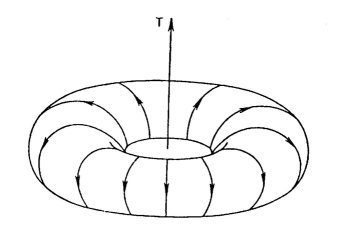
Figure 1: Current configuration with a toroidal dipole moment. The arrows on the torus indicate the direction of the current, and the TDM is directed towards the symmetry axis of the torus.

The simplest TDM model (anapole) was given by Zel’dovich as a conventional solenoid rolled up in a torus and with only one poloidal current, see fig. 1. For such stationary solenoid, without azimuthal components for the current or the electric field, there is only one magnetic azimuthal field different from zero inside the torus.

4 One-loop calculation

The TDM of the neutralino may be defined in the one-loop approximation in the cMSSM by the Feynman diagrams shown in figs. 2 and 3, where $f$ represents the charged fermions of the SM. Taking each fermionic family separately we obtain 94 Feynman diagrams in total: 66 corresponding to self-energy and 28 to vertex corrections.

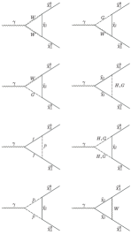
Figure 2: One-loop vertex corrections to the process $\gamma\longrightarrow\chi_{1}^{0}\chi_{1}^{0}$.

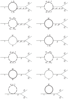
Figure 3: One-loop corrections to the self-energy for the process $\gamma\longrightarrow\chi_{1}^{0}\chi_{1}^{0}$.

We use FeynCalc to calculate the amplitude of these diagrams. Since we are only interested in the terms that contribute to the anapole form factor, we isolate the ones that have the Lorentz structure $\gamma_{\mu}\gamma_{5}$. It is important to notice here that we work in the t’Hooft-Feynman gauge ($\xi=1$). One of the first results we obtain is that the self-energies $\gamma H^{0}$, $\gamma h^{0}$, $\gamma A^{0}$ and $\gamma G^{0}$ do not contribute to the calculation. If we call $\Xi_{i}$ the coefficient that multiplies $\gamma_{\mu}\gamma_{5}$ for the ith diagram, then we have that

$$\sum_{i}\Xi_{i}=f_{A}(q^{2})q^{2}.$$ (7)

To obtain the toroidal dipole moment $\tau=f_{A}(0)$ we use the l’Hopital rule and get

$$\tau=f_{A}(0)=\lim_{q^{2}\rightarrow 0}\frac{\sum_{i}\Xi_{i}}{q^{2}}=\frac{\partial\sum_{i}\Xi_{i}}{\partial q^{2}}\mid_{q^{2}\rightarrow 0}.$$ (8)

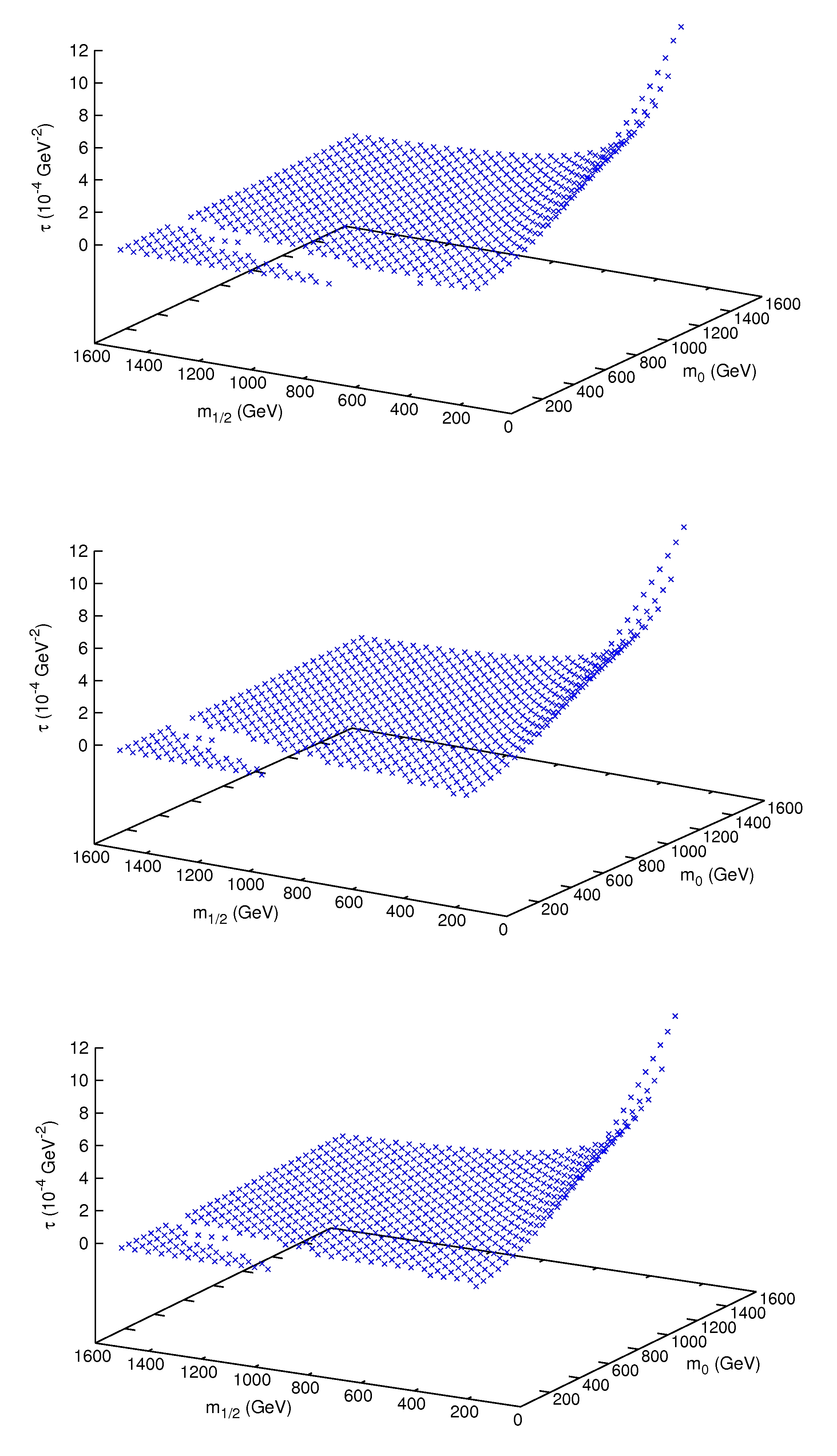
Figure 4: TDM for $\tan\beta=10$, ${\rm sign}\mu=+$ y $A_{0}=-1000$ (top), $0$ (centre) y $1000$ (bottom) GeV.

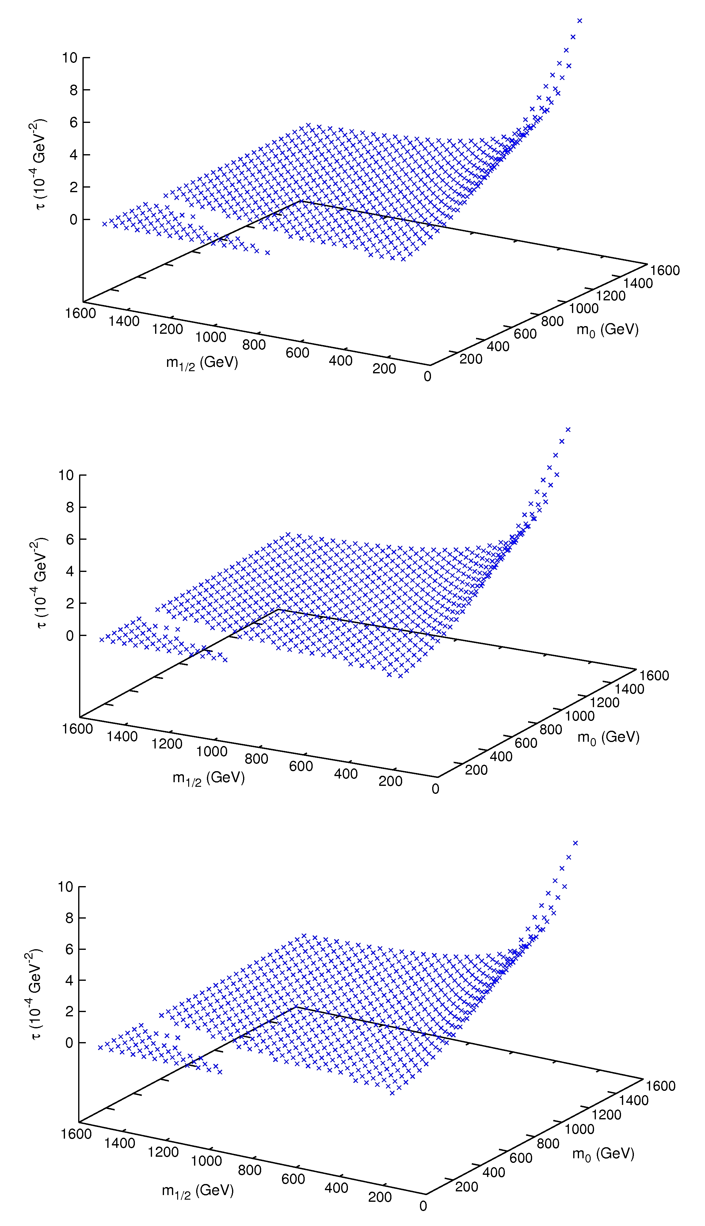
Figure 5: TDM for $\tan\beta=10$, ${\rm sign}\mu=-$ y $A_{0}=-1000$ (top), $0$ (centre) y $1000$ (bottom) GeV.

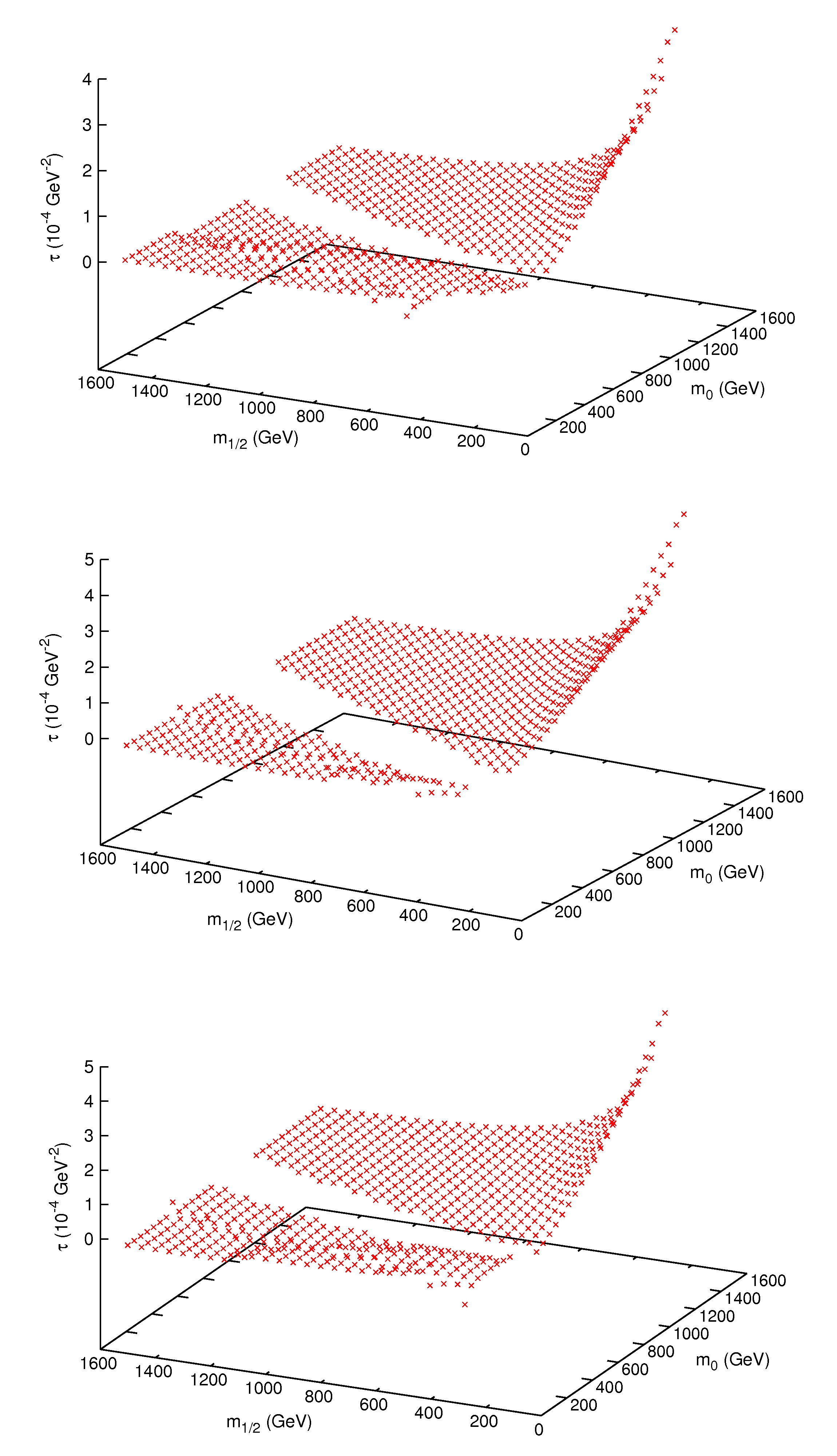
Figure 6: TDM for $\tan\beta=50$, ${\rm sign}\mu=+$ y $A_{0}=-1000$ (top), $0$ (centre) y $1000$ (bottom) GeV.

The contributions to the self-energies have two point Passarino-Veltman scalar functions of the type $B_{0}\left(q^{2},x^{2},x^{2}\right)$ and $B_{0}\left(0,x^{2},x^{2}\right)$. Likewise, the contributions to the vertex corrections have two and three point scalar functions of the type $B_{0}\left(q^{2},x^{2},x^{2}\right)$, $B_{0}\left(M^{2}_{\tilde{\chi}_{1}^{0}},y^{2},x^{2}\right)$ and $C_{0}\left(q^{2},M^{2}_{\tilde{\chi}_{1}^{0}},M^{2}_{\tilde{\chi}_{1}^{0}},x^{2},x^{2},y^{2}\right)$. In both cases $x$ and $y$ represent the masses of the particles in the loop.

When evaluating (6), derivatives of the Passarino-Veltman functions appear. To evaluate the $B_{0}$’s, as well as their derivatives, we use LoopTools[35]. To evaluate the $C_{0}$’s and their derivatives we expande them in a power series around $q^{2}=0$ (see appendix).

The expression obtained for the toroidal dipole moment depends on various parameters of the MSSM, including the supersymmetric particles masses as well as the mass mixing matrix elements, the value of $\tan\beta$, and the values of the soft breaking terms. We evaluate the TDM within the cMSSM using Suspect[36], by fixing the value of $A_{0}$, $\tan\beta$ and ${\rm sign}\mu$, and scanning over the other two parameters $m_{0}$ and $m_{1/2}$, from $0$ to $1500$ GeV and $250$ to $1500$ GeV, respectively.

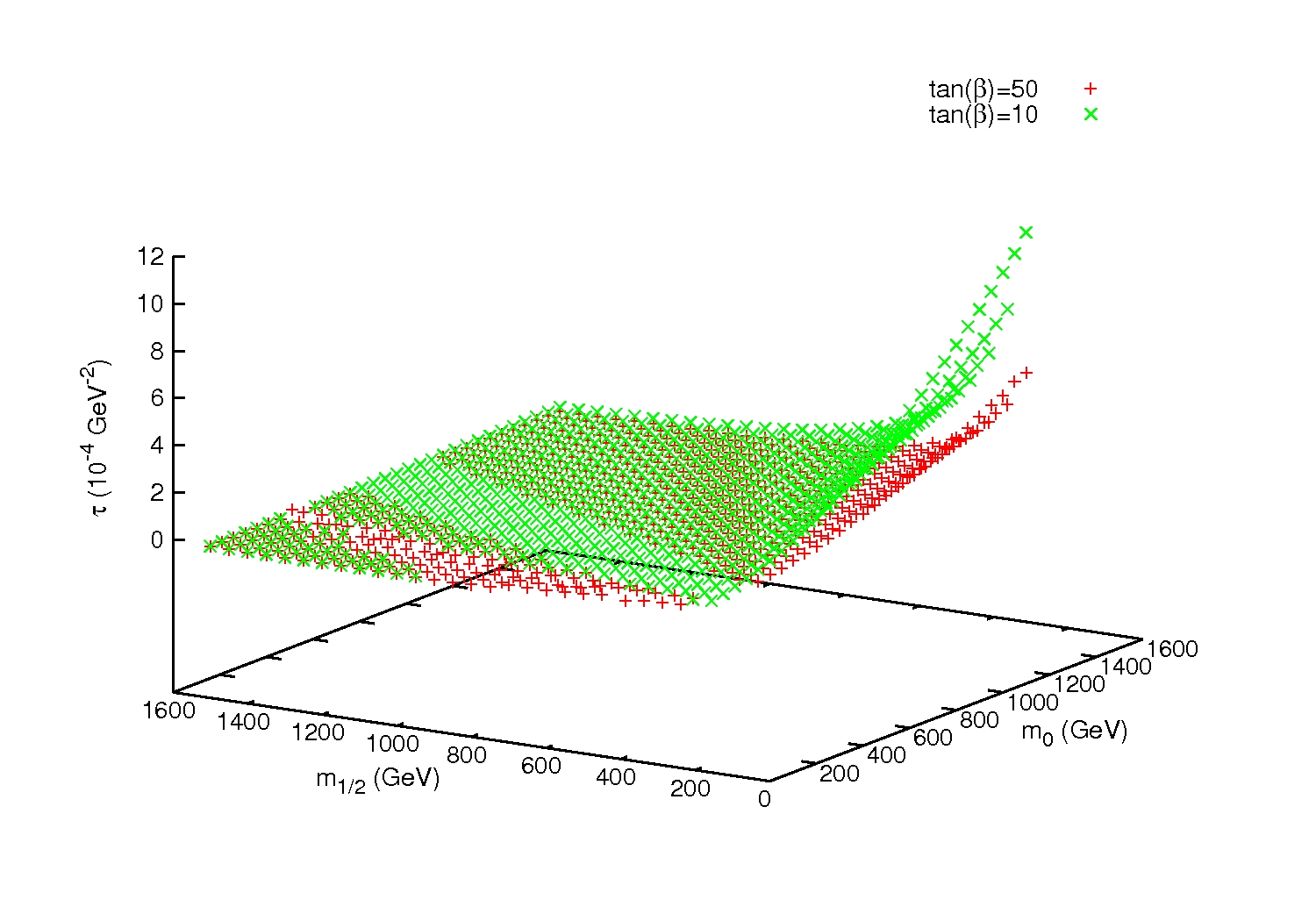
Figure 7: TDM for ${\rm sign}\mu=+$, $A_{0}=0$ GeV, $\tan\beta=10$ (green) and $\tan\beta=50$ (red).

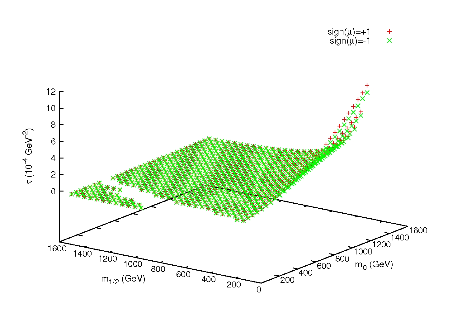
Figure 8: TDM for $\tan\beta=10$, $A_{0}=0$ GeV, ${\rm sign}\mu=+$ (red) and ${\rm sign}\mu=-$ (green).

Figure 4 shows the neutralino toroidal dipole moment for $\tan\beta=10$, $\mu>0$, and three different values of $A_{0}$, $-1000$, $0$ and $1000$ GeV (top to bottom). Comparing the three different plots, no dependence on $A_{0}$ is shown. The TDM is very low for almost every region of the parameter space scanned, with values between $10^{-5}$ and $10^{-8}$ GeV^-2. However the TDM increases for increasing $m_{0}$ and decreasing $m_{1/2}$, reaching values over $10^{-3}$ GeV^-2 for high $m_{0}$ ($\geq 800$ GeV) and low $m_{1/2}$ ($\leq 400$ GeV). Similarly, figure 6 shows the results for $\tan\beta=50$, $\mu>0$, and the same three different values of $A_{0}$, $-1000$, $0$ and $1000$ GeV (top to bottom). The TDM reaches values around $10^{-3}$ GeV^-2.

Figure 5 shows the TDM for $\tan\beta=10$ and $\mu<0$. Sign$\mu>0$ may solve the problem of the discrepancy between the measured value of $g-2$ of the muon and the one predicted by the SM. However, this does not mean negative sign$\mu$ is ruled out since others mechanisms could solve this problem, and therefore sign$\mu<0$ should be taken into consideration.

Figure 7 shows a comparison of two plots for different $\tan\beta$ but same sign$\mu$ and $A_{0}$. This figure shows the dependence of the TDM on $\tan\beta$. Figure 8 shows a comparison of two plots for different values of sign$\mu$ but same $\tan\beta$ and $A_{0}$. This figure shows no dependence of the TDM on sign$\mu$.

Notice that in all the plots the region for which $M_{\tilde{\chi}_{1}^{0}}=M_{\tilde{\tau}}$ is suppressed since we are not considering this possibility. This condition ($M_{\tilde{\chi}_{1}^{0}}=M_{\tilde{\tau}}$) separates the region where the neutralino $\tilde{\chi}_{1}^{0}$ is the LSP and the one where the stau $\tilde{\tau}$ is the LSP.

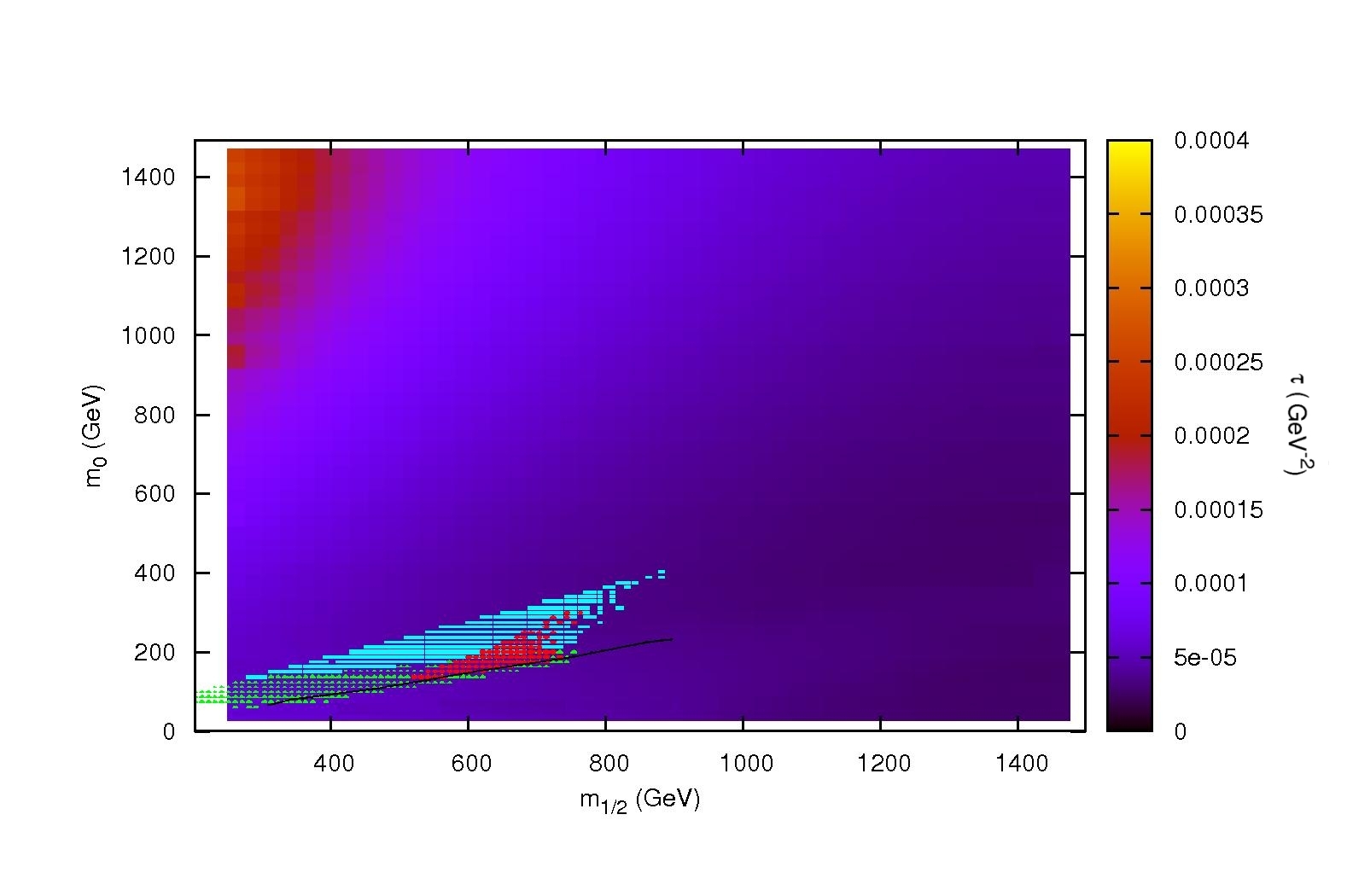
Figure 9: TDM results for $\tan\beta=10$, $A_{0}=0$ GeV and ${\rm sign}\mu=+$ combined with restrictions from cosmological observational data (WMAP).

If combined with other criteria, our results can be used to further reduce the parameter space of the cMSSM. As an example, figure 9 combines our results with those obtained in ref. [37]. They studied the allowed parameter space for diferent models (including cMSSM), supposing that the neutralino is the main component of the CDM, varying $A_{0}$ and imposing the restrictions of cosmological experimental data from WMAP. As can be seen in the plot, their criteria favours a region with very low $m_{0}$, which is compatible with a TDM $<10^{-5}$ GeV^-2 for the neutralino. In other words, if a TDM is measured for a WIMP and it is around or higher than $10^{-4}$ GeV, the neutralino of the cMSSM would no longer be a good candidate for CDM in this region of parameter space.

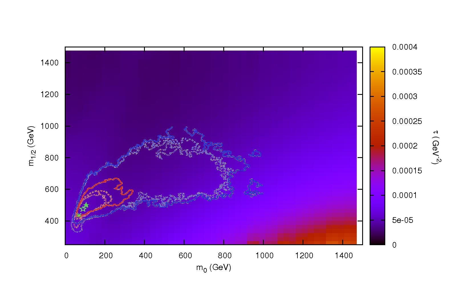
Figure 10: TDM results for $\tan\beta=10$, $A_{0}=0$ GeV, ${\rm sign}\mu=+$ combined with restrictions from initial direct LHC searches for supersymmetry.

In figure 10 we compare our results with a frequentist analysis of the probable ranges of parameters of the MSSM using the results of initial direct LHC searches for supersymmetry, combined with the required cold dark matter density, and the spin-independent dark matter scattering cross section [38]. The figure shows the 68 and 95% CL contours (red and blue, respectively) both after applying the CMS and ATLAS constrains (dashed and solid lines, respectively) and beforehand (dotted lines), taken from their paper. Also shown in the figure as open (solid) green stars are the best-fit points found after applying the CMS (ATLAS) constrainsts in the cMSSM. As can be seen in the figure, this analysis also favours a neutralino with a very low TDM.

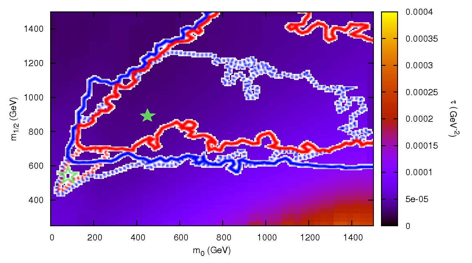
Figure 11: TDM results for $\tan\beta=10$, $A_{0}=0$ GeV, ${\rm sign}\mu=+$ combined with restrictions from searches for supersymmetric signals using $~{}1/$fb of LHC data.

In figure 11 we compare our results with another frequentist analysis of the CMSSM pararameter space including the public results of searches for supersymmetric signals using $~{}1/$fb of LHC data recorded by ATLAS and CMS and $~{}0.3/$fb of data recorded by LHCb in addition to electroweak precision and B-physics obsevables [39]. The figure shows the 68 and 95% CL contours (red and blue, respectively) with LHC_1/b data (solid lines) and showing pre-LHC fits (dotted lines), taken from their paper. Although this analysis widens the allowed parameter space, it still favours a neutralino with very low TDM.

5 Conclusions

We calculated the only electromagnetic property of the lightest neutralino: its toroidal dipole moment. Its characterization is extremely valuable for discriminating different models which have the neutralino as dark matter candidate. We performed the calculation in the framework of the cMSSM, however a similar analysis can be performed for other models (work in progress). We found that the TDM of the neutralino is highly sensitive to $m_{0}$, $m_{1/2}$ and $\tan\beta$, but very weakly or practically non-dependent on $A_{0}$ and sign$\mu$.

All points in the parameter space we scanned give a TDM consistent with the upper limit ($\sim 10^{-2}$ GeV^-2) obtained by Pospelov and ter Veldhuis [24] for WIMPs interacting with heavy nuclei using data from the CDMS and DAMA experiments. However, this data can and will be improved in the next few years helping to refine the upper limit, likely ruling out some regions of the parameter space.

The TDM analysis can be used as another criteria to constrain the parameter space of a given model which has a neutralino as candidate for dark matter. Thus, according to our results, if a non-zero (around $10^{-4}$-$10^{-3}$ GeV^-2) TDM could be measured for the neutralino, that would indicate that the favored region of the parameter space of the cMSSM would be high $m_{0}$ ($\geq 800$ GeV) and low $m_{1/2}$ ($\leq 400$ GeV). Otherwise, other regions are compatible with a TDM lower than $10^{-5}$ GeV.

If combined with other criteria (such as dark matter relic density, or frequentist analysis of data from the LHC) the parameter space can be reduced even further. In fact, the combination with these other criteria favours a region with low $m_{0}$, which is compatible with a $10^{-5}$-$10^{-8}$ GeV^-2 TDM for the neutralino. This means, among other things, that if a TDM higher than $10^{-4}$ GeV^-2 is measured for a WIMP it would exclude some regions of parameter space of the cMSSM (and other more specific models), at least if the neutralino is the only component of dark matter. One should keep in mind that all analysis mentioned were made with this assumption.

6 Acknowledgements

We acknowledge very useful discussions with E. Ley Koo and A. Mondragón.
This work was partially supported by UNAM grants PAPIIT IN111609 and IN113412.

Appendix: Scalar Three-point Function

In this appendix, we analyse the Passarino-Veltman scalar three-point function $C_{0}(q^{2},x^{2},x^{2},z^{2},z^{2},y^{2})$ [40, 41] which appears in the TDM calculation. Here $q^{2}$ denotes the photon transfered 4-momentum, $x$ is the neutralino mass, and $y$ and $z$ are the masses of the particles running in the loop.

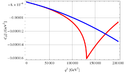
Figure 12: Comparison between numerical (red line) and approximate (blue line) scalar three-point function $C_{0}(q^{2},x^{2},x^{2},z^{2},z^{2},y^{2})$, with $x=97.7$ GeV, $y=415.4$ GeV and $z=80.43$ GeV. The analytical approximation (blue line) is only valid for $q^{2}\rightarrow 0$.

The corresponding plot for this $C_{0}$ function can be seen in figure 12. The red line shows the numerical solution, the blue line line represents the approximate solution, i.e., the Taylor expansion around $q^{2}=0$, which can be written as follows:

$$C_{0}\left(q^{2},x^{2},x^{2},z^{2},z^{2},y^{2}\right)=\alpha_{0}+\alpha_{1}q^{2}+{\cal O}(q^{4}).$$ (9)

The coefficients $\alpha_{i}$ are functions of the masses:

$$\alpha_{0}=\frac{\log\left(\frac{y^{2}}{z^{2}}\right)}{2x^{2}}+a\log\omega,$$ (10)

$$\alpha_{1}=\frac{x^{4}-y^{2}x^{2}-2z^{2}x^{2}+z^{4}-y^{2}z^{2}}{6x^{2}z^{2}(-x+y-z)(x+y-z)(-x+y+z)(x+y+z)}+\frac{\log\left(\frac{y^{2}}{z^{2}}\right)}{12x^{4}}+b\log\omega,$$ (11)

where

$$\omega=\frac{\left(ix^{2}+iy^{2}-iz^{2}+\sqrt{-y^{4}+2(x^{2}+z^{2})y^{2}-(z^{2}-x^{2})}\right)\left(ix^{2}-iy^{2}+iz^{2}+\sqrt{-y^{4}+2(x^{2}+z^{2})y^{2}-(z^{2}-x^{2})}\right)}{\left(-ix^{2}+iy^{2}-iz^{2}+\sqrt{-y^{4}+2(x^{2}+z^{2})y^{2}-(z^{2}-x^{2})}\right)\left(-ix^{2}-iy^{2}+iz^{2}+\sqrt{-y^{4}+2(x^{2}+z^{2})y^{2}-(z^{2}-x^{2})}\right)},$$ (12)

$$a=\frac{i(x^{2}+y^{2}-z^{2})}{2x^{2}\sqrt{-x^{4}+2y^{2}x^{2}+2z^{2}x^{2}-y^{4}-z^{4}+2y^{2}z^{2}}}$$ (13)

and

$$b=\frac{i(x^{2}+y^{2}-z^{2})(x^{4}-4y^{2}x^{2}-2z^{2}x^{2}+y^{4}+ź^{4}-2y^{2}z^{2})}{12x^{4}(-x+y-z)(x+y-z)(-x+y+z)(x+y+z)\sqrt{-x^{4}+2y^{2}x^{2}+2z^{2}x^{2}-y^{4}-z^{4}+2y^{2}z^{2}}}.$$ (14)

References

- [1] A. M. Szelc, Acta Phys.Polon. B41, 1417 (2010), [1010.3918].
- [2] R. Schnee, 1101.5205.
- [3] K. Sigurdson, M. Doran, A. Kurylov, R. R. Caldwell and M. Kamionkowski, Phys.Rev. D70, 083501 (2004), [astro-ph/0406355].
- [4] P. Ciafaloni et al., JCAP 1103, 019 (2011), [1009.0224].
- [5] P. Ciafaloni and A. Urbano, Phys.Rev. D82, 043512 (2010), [1001.3950].
- [6] P. Ciafaloni et al., 1104.2996.
- [7] N. F. Bell, J. B. Dent, T. D. Jacques and T. J. Weiler, Phys.Rev. D83, 013001 (2011), [1009.2584].
- [8] N. F. Bell, J. B. Dent, T. D. Jacques and T. J. Weiler, 1101.3357.
- [9] N. F. Bell et al., 1104.3823.
- [10] J. B. Dent, R. J. Scherrer and T. J. Weiler, Phys.Rev. D78, 063509 (2008), [0806.0370].
- [11] M. Kachelriess, P. Serpico and M. Solberg, Phys.Rev. D80, 123533 (2009), [0911.0001].
- [12] J. H. Heo, 0902.2643.
- [13] J. H. Heo, Phys.Lett. B693, 255 (2010), [0901.3815].
- [14] S. Liebler and W. Porod, Nucl.Phys. B849, 213 (2011), [1011.6163], * Temporary entry *.
- [15] V. Barger, W.-Y. Keung and D. Marfatia, Phys.Lett. B696, 74 (2011), [1007.4345].
- [16] V. Berezinsky, M. Kachelriess and S. Ostapchenko, Phys.Rev.Lett. 89, 171802 (2002), [hep-ph/0205218].
- [17] M. Kachelriess and P. Serpico, Phys.Rev. D76, 063516 (2007), [0707.0209].
- [18] Y. Zeldovich, Zh. Eksp. Teor. Fiz 33, 1531 (1957).
- [19] G. N. Afanasev and V. M. Dubovik, Sov. J. Part. Nucl. 23, 552 (1992).
- [20] G. N. Afanasev, V. M. Dubovik and S. Misicu, J. Phys. A26, 3279 (1993).
- [21] V. M. Dubovik and V. E. Kuznetsov, Int. J. Mod. Phys. A13, 5257 (1998), [hep-ph/9606258].
- [22] E. N. Bukina, V. M. Dubovik and V. E. Kuznetsov, Phys.Lett. B435, 134 (1998), [hep-ph/9805491].
- [23] A. Gongora and E. Ley-Koo, Rev. Mex. Fis. E 52, 188 (2006).
- [24] M. Pospelov and T. ter Veldhuis, Phys. Lett. B480, 181 (2000), [hep-ph/0003010].
- [25] R. Bernabei et al., Phys. Lett. B389, 757 (1996).
- [26] CDMS, R. Abusaidi et al., Phys. Rev. Lett. 84, 5699 (2000), [astro-ph/0002471].
- [27] WMAP Collaboration, E. Komatsu et al., Astrophys.J.Suppl. 192, 18 (2011), [1001.4538].
- [28] G. Jungman, M. Kamionkowski and K. Griest, Phys.Rept. 267, 195 (1996), [hep-ph/9506380].
- [29] K. A. Olive, astro-ph/0301505.
- [30] J. L. Feng, Ann.Rev.Astron.Astrophys. 48, 495 (2010), [1003.0904].
- [31] S. P. Martin, hep-ph/9709356.
- [32] I. J. Aitchison, hep-ph/0505105, Notes of Lectures for Graduate Students in Particle Physics Oxford, 2004 and 2005.
- [33] E. N. Bukina, V. M. Dubovik and V. E. Kuznetsov, JINR-E4-98-95.
- [34] V. Dubovik and A. Cheshkov, Sov. J. Particles Nucl. 5, 318 (1975).
- [35] T. Hahn and M. Perez-Victoria, Comput. Phys. Commun. 118, 153 (1999), [hep-ph/9807565].
- [36] A. Djouadi, J.-L. Kneur and G. Moultaka, Comput. Phys. Commun. 176, 426 (2007), [hep-ph/0211331].
- [37] L. S. Stark, P. Hafliger, A. Biland and F. Pauss, JHEP 0508, 059 (2005), [hep-ph/0502197].
- [38] O. Buchmueller et al., Eur. Phys. J. C71, 1634 (2011), [1102.4585].
- [39] O. Buchmueller et al., Eur.Phys.J. C72, 1878 (2012), [1110.3568], 25 pages, 36 figures.
- [40] L. G. Cabral-Rosetti and M. A. Sanchiz-Lozano, J.Comput.Appl.Math. 115, 93 (2000), [hep-ph/9809213].
- [41] L. G. Cabral-Rosetti and M. A. Sanchiz-Lozano, J.Phys.Conf.Ser. 37, 82 (2006), [hep-ph/0206081].