Two-Nucleon Scattering without partial waves using a momentum space Argonne V18 interaction

Abstract

We test the operator form of the Fourier transform of the Argonne V18 potential by computing selected scattering observables and all Wolfenstein parameters for a variety of energies. These are compared to the GW-DAC database and to partial wave calculations. We represent the interaction and transition operators as expansions in a spin-momentum basis. In this representation the Lippmann-Schwinger equation becomes a six channel integral equation in two variables. Our calculations use different numbers of spin-momentum basis elements to represent the on- and off-shell transition operators. This is because different numbers of independent spin-momentum basis elements are required to expand the on- and off-shell transition operators. The choice of on and off-shell spin-momentum basis elements is made so that the coefficients of the on-shell spin-momentum basis vectors are simply related to the corresponding off-shell coefficients.

I Introduction

Among the so-called ‘high precision’ nucleon-nucleon (NN) potentials the Argonne V18 potential Wiringa et al. (1995) is the only one given in a basis of spin-isospin operators, $O_{n}$, which are multiplied by scalar functions, $V_{n}(r)$, of the relative distance $r$. These features are advantageous for some applications, however, there are classes of problems where a momentum-space treatment is preferred. These applications include relativistic few-nucleon scattering and electroweak probes of few-nucleon systems. While realistic momentum-space nucleon-nucleon potentials are available, they are either given in terms of partial-wave expansions, e.g. the CD-Bonn interaction Machleidt (2001) and the Nijmegen interaction Stoks et al. (1994), or they are limited to low energies, like the interactions derived in chiral effective field theory Epelbaum et al. (2005); Entem and Machleidt (2003).

The experience in standard three-nucleon calculations that is based on a partial-wave projected momentum-space basis Gloeckle et al. (1996) shows that while this standard treatment is quite successful at lower energies, the numerical realization of the scattering equations becomes more tedious with increasing energy. For a system of three bosons interacting via scalar forces it already has been demonstrated that it is relatively easy to directly calculate three-body scattering observables in a relativistic Faddeev scheme without using partial wave projections  Lin et al. (2008, 2008). Thus, it is natural to strive for solving the three-nucleon Faddeev equations in a similar fashion.

The first step in this direction is solving the two-nucleon problem based on an operator expansion instead of a partial-wave projected momentum-space basis. One of the advantages of using operator expansions over partial waves is that the transition matrix elements are reasonably smooth. At higher energies, an accurate representation of these smooth, but forward-peaked, functions requires a large number of partial waves. A converged partial-wave expansion of the transition matrix elements implies that all of the high-frequency oscillations from the large-$l$ partial waves must largely cancel. In addition, to achieve these cancellations the computation of the transition matrix elements requires the accurate computation of oscillatory integrals. At low-energies partial waves are preferred because they replace the two-variable Lippmann-Schwinger equation by a finite set of uncoupled one-variable equations. For sufficiently high energies the simplicity of a direct vector treatment of the Lippmann-Schwinger equation has advantages, even though the integral equation has an additional integration variable. In this paper we discuss the direct vector solution of the Lippmann-Schwinger equation using a recent momentum-space treatment of the Argonne V18 potential Veerasamy and Polyzou (2011). There the potential was only tested in the calculation of the deuteron bound state, which is not sensitive to the charge symmetry breaking parts of the AV18 potential. Solving for the scattering observables provides a complete test of the momentum-space representation of the AV18 potential presented in Refs. Veerasamy and Polyzou (2011); Veerasamy (2011).

There have been several approaches formulating nucleon-nucleon (NN) scattering without employing a partial-wave decomposition. A helicity formulation related to the total NN spin was proposed in Fachruddin et al. (2000). The spectator equation for relativistic NN scattering has been successfully solved in Ramalho et al. (2006), also using a helicity formulation.

A three-dimensional formulation based on an operator expansion was proposed and carried out for a chiral next-to-next-leading order NN force and a standard one-boson-exchange potential in  Golak et al. (2010). A basic foundation for the latter rests on the fact that the most general form of the NN interaction can be represented as a linear combination of six linearly-independent spin-momentum operators with scalar coefficient functions. This representation determines the spin-structure of the NN bound and scattering states. The Wolfenstein decomposition of the NN scattering amplitude into five linear operators is dictated by rotational, space reflection, spin-exchange symmetry, and time-reversal invariance Wolfenstein and Ashkin (1952). A sixth independent operator with these symmetries does not exist on shell. Ref. Golak et al. (2010) uses six linearly independent operators that satisfy all of the symmetry requirements, but these operators become linearly dependent on shell so the scattering amplitude was computed from the off-shell result by the required continuity of the transition matrix elements.

The vector treatment of the spins requires the computation of an analytic expression for each spin-basis element at each quadrature point. A symbolic reduction technique, developed in  Veerasamy (2011), automates the computation of these expressions. Our calculations use five independent spin-operators to expand the on-shell transition matrix element and an additional sixth operator to expand the off-shell transition matrix elements. Based on calculations using different choices of the sixth operator, we find that using a sixth operator that changes sign under time reversal to expand the off-shell transition matrix elements leads to a numerically more stable discretization of the Lippmann-Schwinger equation when compared to calculations using a sixth operator that has the symmetries of the potential. An important observation is that while a time-odd operator appears in the expansion of the potential, the potential itself remains invariant with respect to time reversal because the expansion coefficients also contain time-odd components. The expansion coefficient of the time-odd operator that we consider vanishes on-shell.

In Sec. II we discuss the operator basis that we use to expand the NN potential and derive in Sec. III the resulting Lippmann-Schwinger equation and show how we explicitly obtain the on-shell scattering amplitude. We then discuss our numerical procedure and the extraction of the Wolfenstein amplitudes in Sec. IV. In Sec. V we discuss the selected NN observables at different energies, and conclude in Sec. VI.

II Operator Expansions

Momentum-space scattering calculations are performed using the Lippmann-Schwinger integral equation. It is a singular integral equation with a compact kernel. This means that the kernel can be uniformly approximated by a finite dimensional matrix and that the equations can be solved to any desired accuracy by solving a finite system of linear equations.

The Lippmann-Schwinger equation has the well-known form

$$T(z)=V+V(z-H_{0})^{-1}T(z).$$ (1)

We represent the operators in this equation by matrix elements in the total momentum $\mathbf{P}$ and single-particle momentum, $\mathbf{p}=\frac{1}{2}(\mathbf{p}_{p}-\mathbf{p}_{n})$, boosted to the system rest frame with a Galilean boost. Matrix element of the interaction and transition operator have the form

$$\langle\mathbf{P}^{\prime},\mathbf{p}^{\prime}|V|\mathbf{P},\mathbf{p}\rangle=\delta(\mathbf{P}^{\prime}-\mathbf{P})\langle\mathbf{p}^{\prime}\|V\|\mathbf{p}\rangle$$ (2)

and

$$\langle\mathbf{P}^{\prime},\mathbf{p}^{\prime}|T(z)|\mathbf{P},\mathbf{p}\rangle=\delta(\mathbf{P}^{\prime}-\mathbf{P})\langle\mathbf{p}^{\prime}\|T(z)\|\mathbf{p}\rangle,$$ (3)

where the reduced matrix elements $\langle\mathbf{p}^{\prime}\|V\|\mathbf{p}\rangle$ and $\langle\mathbf{p}^{\prime}\|T(z)\|\mathbf{p}\rangle$ are matrices in spin-isospin space.

Any operator $V$ on the two-nucleon Hilbert space can be expanded as a linear combination of the spin-basis operators, $\Sigma_{\mu\nu}:=\sigma_{1\mu}\otimes\sigma_{2\nu}$, where $\sigma_{i\mu}=(I,\boldsymbol{\sigma})$,

$$V=\sum V^{\mu\nu}\Sigma_{\mu\nu}$$ (4)

and

$$V^{\mu\nu}=\frac{1}{4}Tr(\Sigma_{\mu\nu}V).$$ (5)

The operator $\Sigma_{\mu\nu}$ has sixteen components, however the number of independent operator types that can appear in a transition operator or potential is constrained by rotational invariance, time-reversal invariance, space-reflection symmetry, and spin-exchange symmetry. Spin-exchange symmetry means that the potential commutes with the square of the total spin, which is a symmetry of nucleon-nucleon interactions. These symmetries can be utilized to reduce number of coupled Lippmann-Schwinger equations.

The three Pauli spin matrices in $\Sigma_{\mu\nu}$ for each particle can be replaced by the rotationally invariant operators, $\mathbf{\hat{{V}}_{i}}\cdot\boldsymbol{\sigma}_{j}$, for any independent set of vector operators, $\{\mathbf{\hat{{V}}_{1}},\mathbf{\hat{{V}}_{2}},\mathbf{\hat{{V}}_{3}}\}$. The traces of the product of these operators with the potential have the same time-reversal, space-reflection, and spin-exchange symmetry as the operators. If the spin operators are chosen to be orthonormal with respect to the trace norm, the only operators that contribute to the potential expansion are the operators that satisfy all these symmetries, except time-reversal invariance, because it is possible to have a scalar coefficient function that changes sign on time reversal. Consideration of the symmetries of a complete set of spin operators implies that the most general interaction consistent with these symmetries can be represented by an expansion in terms of five operators on shell and six off shell. When the spin operators are not orthonormal with respect to the trace, a matrix inversion is needed to compute the expansion of the potential. This inverse matrix may not have any simple symmetry with respect to time reversal. The same will be true for the resulting expansion coefficients. Nevertheless, the number of operators needed is unchanged and the symmetries of the full potential are preserved.

In this paper we consider the following independent momentum operators used by Wolfenstein Wolfenstein (1954)

$$\hat{\mathbf{K}} := {(\mathbf{p}^{\prime}-\mathbf{p})\over|\mathbf{p}^{\prime}-\mathbf{p}|}$$ (6)

$$\hat{\mathbf{Q}} := {(\mathbf{p}^{\prime}+\mathbf{p})\over|\mathbf{p}^{\prime}+\mathbf{p}|}$$ (7)

$$\hat{\mathbf{N}} := {(\mathbf{p}^{\prime}\times\mathbf{p})\over|\mathbf{p}^{\prime}\times\mathbf{p}|}.$$ (8)

These vector operators can be classified by their transformation properties with respect to space reflection and time reversal.

A useful independent set of spin operators that are sufficient to expand the scattering amplitude matrix $M$ was given by Wolfenstein. In terms of the vectors of Eq. (8) the Wolfenstein operators are

$$\Big{\{}I,(\mbox{\boldmath$\sigma$}_{1}\cdot\hat{\mathbf{Q}})\otimes(\mbox{\boldmath$\sigma$}_{2}\cdot\hat{\mathbf{Q}}),(\mbox{\boldmath$\sigma$}_{1}\otimes I+I\otimes\mbox{\boldmath$\sigma$}_{2})\cdot\hat{\mathbf{N}},(\mbox{\boldmath$\sigma$}_{1}\cdot\hat{\mathbf{N}})\otimes(\mbox{\boldmath$\sigma$}_{2}\cdot\hat{\mathbf{N}}),(\mbox{\boldmath$\sigma$}_{1}\cdot\hat{\mathbf{K}})\otimes(\mbox{\boldmath$\sigma$}_{2}\cdot\hat{\mathbf{K}})\Big{\}}.$$ (9)

The coefficients of the expansion of the scattering amplitude matrix in Wolfenstein spin-operators are the so-called Wolfenstein parameters, $a,c,m,g,h$. Knowledge of these parameters as a function of the initial and final momenta contains all of the information in the scattering amplitude matrix. The scattering-amplitude matrix is related to the on-shell transition matrix element by

$$M(\mathbf{p}^{\prime},\mathbf{p})=-4\pi^{2}\mu\langle\mathbf{p}^{\prime}\|T(z)\|\mathbf{p}\rangle$$ (10)

where $\mu$ is the reduced mass of the two-nucleon system and the Wolfenstein parameterization of $M(\mathbf{p}^{\prime},\mathbf{p})$ is

$$M = aI+c(\mbox{\boldmath$\sigma$}_{1}\otimes I+I\otimes\mbox{\boldmath$\sigma$}_{2})\cdot\hat{\mathbf{N}}+m(\mbox{\boldmath$\sigma$}_{1}\cdot\hat{\mathbf{N}})\otimes(\mbox{\boldmath$\sigma$}_{2}\cdot\hat{\mathbf{N}})+$$ (12)

$$(g+h)(\mbox{\boldmath$\sigma$}_{1}\cdot\hat{\mathbf{Q}})\otimes(\mbox{\boldmath$\sigma$}_{2}\cdot\hat{\mathbf{Q}})+(g-h)(\mbox{\boldmath$\sigma$}_{1}\cdot\hat{\mathbf{K}})\otimes(\mbox{\boldmath$\sigma$}_{2}\cdot\hat{\mathbf{K}}).$$

The operators of Eq. (12) are invariant with respect to rotations, space reflection, spin exchange, and time reversal.

The additional operator,

$$(\mbox{\boldmath$\sigma$}_{1}\cdot\hat{\mathbf{K}})\otimes(\mbox{\boldmath$\sigma$}_{2}\cdot\hat{\mathbf{Q}})+(\sigma_{1}\cdot\hat{\mathbf{Q}})\otimes(\mbox{\boldmath$\sigma$}_{2}\cdot\hat{\mathbf{K}}),$$ (13)

is rotationally invariant, space reflection invariant and spin exchange invariant, but changes sign under time reversal. If this operator is paired with a coefficient function that also changes sign under time reversal then the product is invariant with respect to time reversal. A time-odd coefficient function must be odd in $|\mathbf{p}^{\prime}|^{2}-|\mathbf{p}|^{2}$, and thus vanish on shell. This means that while this operator cannot appear in the scattering amplitude matrix, $M$, it can appear in the interaction or half-shell transition matrix and it may also appear in the off-shell unitarity constraint on the transition operator.

The six independent operators of Eqs. (9) and (13) are sufficient to expand any potential that is invariant with respect to rotations, space reflection, time reversal, and spin exchange.

In order to solve the Lippmann-Schwinger equation the interaction is expanded in terms of these six independent spin operators. In our applications the operator $(\mbox{\boldmath$\sigma$}_{1}\cdot\hat{\mathbf{N}})\otimes(\mbox{\boldmath$\sigma$}_{2}\cdot\hat{\mathbf{N}})$ is replaced by the operator $(\mbox{\boldmath$\sigma$}_{1}\cdot\mbox{\boldmath$\sigma$}_{2})$. This replacement is done for numerical reasons, but it is also useful because this operator appears in the spin-spin part of the interaction as well as in the tensor force.

The transition matrix elements can be expanded using the same six operators. This results in a set of six coupled equations for the half-shell or off-shell transition matrix elements. Since the scattering amplitude matrix is related to the on-shell transition operator by a multiplicative scalar, it is useful to put the integral equation in a form where the on-shell points are included in the linear equation. To avoid ambiguities, the on-shell amplitude is expanded using 5 independent spin components. This will be discussed in section IV.

The expansion of both the interactions and transition matrix elements is constructed by taking traces with the six independent spin operators

$$W^{1} := {\bf I}$$ (14)

$$W^{2} := \mbox{\boldmath$\sigma$}_{1}\cdot\mbox{\boldmath$\sigma$}_{2}$$ (15)

$$W^{3} := (\mbox{\boldmath$\sigma$}_{1}\cdot\hat{\mathbf{K}})\otimes(\mbox{\boldmath$\sigma$}_{2}\cdot\hat{\mathbf{K}})$$ (16)

$$W^{4} := (\mbox{\boldmath$\sigma$}_{1}\cdot\hat{\mathbf{Q}})\otimes(\mbox{\boldmath$\sigma$}_{2}\cdot\hat{\mathbf{Q}})$$ (17)

$$W^{5} := i(\mbox{\boldmath$\sigma$}_{1}\otimes{\bf I}+{\bf I}\otimes\mbox{\boldmath$\sigma$}_{2})\cdot\hat{\mathbf{N}}$$ (18)

$$W^{6} := (\mbox{\boldmath$\sigma$}_{1}\cdot\hat{\mathbf{K}})\otimes(\mbox{\boldmath$\sigma$}_{2}\cdot\hat{\mathbf{Q}})+(\mbox{\boldmath$\sigma$}_{1}\cdot\hat{\mathbf{Q}})\otimes(\mbox{\boldmath$\sigma$}_{2}\cdot\hat{\mathbf{K}}).$$ (19)

It follows that

$$V=\sum_{i=1}^{6}U_{i}W^{i},$$ (20)

where

$$U_{i}:=(A^{-1})^{ij}\mathbf{Tr}(W^{j}V)\qquad A^{ij}:=\mathbf{Tr}(W^{i}W^{j}).$$ (21)

Both $T(z)$ and $V$ are matrices in the spin and isospin degrees of freedom and the $W^{j}$ and $A^{ij}$ depend on $\mathbf{p}$ and $\mathbf{p}^{\prime}$. By taking traces, the Lippmann-Schwinger equation becomes a set of six coupled integral equations in two variables.

As discussed before, six linearly independent operators are required to expand any NN potential. This expansion can include the product of a time-odd, space reflection invariant spin-momentum operator with a space reflection invariant, time-odd coefficient function resulting in a term that conserves the symmetry properties of the NN-potential. Note that a space-reflection odd operator cannot appear in this expansion because it would require a pseudo-scalar coefficient which cannot be constructed from two vectors Veerasamy (2011).

The spin-spin operator, $W^{2}$, and the Wolfenstein operator $(\mbox{\boldmath$\sigma$}_{1}\cdot{\bf N})(\mbox{\boldmath$\sigma$}_{2}\cdot{\bf N})$ are independent and have all of symmetries of the potential. They are related by

$$\mbox{\boldmath$\sigma$}_{1}\cdot\mbox{\boldmath$\sigma$}_{2}=$$ (23)

$$R\left(\frac{R^{2}}{{(K^{2}Q^{2}-R^{2})}^{2}}-\frac{K^{2}Q^{2}}{{(K^{2}Q^{2}-R^{2})}^{2}}\right)\;\left((\mbox{\boldmath$\sigma$}_{1}\cdot{\bf K})\;(\mbox{\boldmath$\sigma$}_{2}\cdot{\bf Q})+(\mbox{\boldmath$\sigma$}_{1}\cdot{\bf Q})(\mbox{\boldmath$\sigma$}_{2}\cdot{\bf K})\right)$$

$$+ \left(\frac{Q^{2}R^{2}}{{(K^{2}Q^{2}-R^{2})}^{2}}-\frac{K^{2}Q^{4}}{{(K^{2}Q^{2}-R^{2})}^{2}}\right)\;\left(\mbox{\boldmath$\sigma$}_{1}\cdot{\bf K}\right)\left(\mbox{\boldmath$\sigma$}_{2}\cdot{\bf K}\right)+\frac{(\mbox{\boldmath$\sigma$}_{1}\cdot{\bf N})(\mbox{\boldmath$\sigma$}_{2}\cdot{\bf N})}{N^{2}}$$ (24)

$$+ \left(\frac{K^{2}R^{2}}{{(K^{2}Q^{2}-R^{2})}^{2}}-\frac{K^{4}Q^{2}}{{(K^{2}Q^{2}-R^{2})}^{2}}\right)\left(\mbox{\boldmath$\sigma$}_{1}\cdot{\bf Q}\right)\left(\mbox{\boldmath$\sigma$}_{2}\cdot{\bf Q}\right),$$ (25)

which involves $W^{3}$, $W^{4}$ as well as the time-odd operator, $W^{6}$. In this expression $R={\bf K}\cdot{\bf Q}=|\mathbf{p}^{\prime}|^{2}-|\mathbf{p}|^{2}$ is the time-odd coefficient of the time-odd operator $W^{6}$, which vanishes on-shell.

It follows that the basis for the off-shell potential, $W^{1}-W^{6}$ could be replaced by an equivalent basis where $W^{6}$ is replaced by the Wolfenstein operator $(\mbox{\boldmath$\sigma$}_{1}\cdot{\bf N})(\mbox{\boldmath$\sigma$}_{2}\cdot{\bf N})$. While the second basis has all of the symmetries of the potential, the basis that includes the time-odd operator $W^{6}$ is preferable for numerical reasons as will be elaborated on later.

III Lippmann-Schwinger Equations

The reduced transition matrix elements can be expressed as

$$t(p^{\prime},p,x;z):=\langle\mathbf{p}^{\prime}\|T(z)\|\mathbf{p}\rangle\qquad z:=\frac{p_{0}^{2}}{2\mu}+i0^{+},$$ (26)

where the variables are defined below and $t(p^{\prime},p,x;z)$ is a spin-isospin valued function. Here $p_{0}$ represents the on-shell momentum. The Lippmann-Schwinger equation for $t(p^{\prime},p,x;z)$ is the two-variable integral equation

$$t(p^{\prime},p,x^{\prime};z)=$$ (28)

$$v(p^{\prime},p,x^{\prime})+\int_{-1}^{1}dx^{\prime\prime}\int_{0}^{\infty}dp^{\prime\prime}p^{\prime\prime 2}u(p^{\prime},x^{\prime},p^{\prime\prime},x^{\prime\prime})G_{0}(p^{\prime\prime},z)t(p^{\prime\prime},p,x^{\prime\prime};z)\;,$$

where the coordinate system is chosen so that the initial momentum is in the $3$-direction and the scattering plane is the $1$-$3$ plane. The integration over the azimuthal angle only affects variables in the potential and can be carried out independently. The momenta and quantities in Eq. (28) are parameterized in terms of the variables $p,p^{\prime},x^{\prime},p^{\prime\prime},x^{\prime\prime}$ defined by

$$\mathbf{p} := (0,0,p)=\mathbf{p}_{0}$$ (29)

$$\mathbf{p}^{\prime} := \left(p^{\prime}\sqrt{1-x^{\prime 2}},0,p^{\prime}x^{\prime}\right)$$ (30)

$$\mathbf{p}^{\prime\prime} := \left(p^{\prime\prime}\sqrt{1-x^{\prime\prime 2}}\cos(\phi^{\prime\prime}),p^{\prime\prime}\sqrt{1-x^{\prime\prime 2}}\sin(\phi^{\prime\prime}),p^{\prime\prime}x^{\prime\prime}\right)$$ (31)

$$\hat{\mathbf{p}}^{\prime}\cdot\hat{\mathbf{p}} := x^{\prime}$$ (32)

$$\hat{\mathbf{p}}^{\prime\prime}\cdot\hat{\mathbf{p}} := x^{\prime\prime}$$ (33)

$$\hat{\mathbf{p}}^{\prime}\cdot\hat{\mathbf{p}}^{\prime\prime} := y=x^{\prime}x^{\prime\prime}+\sqrt{(1-x^{\prime 2})(1-x^{\prime\prime 2})}\cos(\phi^{\prime\prime})$$ (34)

$$v(p^{\prime},p,x^{\prime}) := V(\mathbf{p}^{\prime},\mathbf{p})$$ (35)

$$v(p^{\prime},p^{\prime\prime},y) := V(\mathbf{p}^{\prime},\mathbf{p}^{\prime\prime})$$ (36)

$$u(p^{\prime},x^{\prime},p^{\prime\prime},x^{\prime\prime},\phi^{\prime\prime}) := v(p^{\prime},p^{\prime\prime},x^{\prime}x^{\prime\prime}+\sqrt{(1-x^{\prime 2})(1-x^{\prime\prime 2})}\cos(\phi^{\prime\prime}))$$ (37)

$$G_{0}(p^{\prime\prime},z) = {2\mu\over p_{0}^{2}-p^{\prime\prime^{2}}+i0^{+}}$$ (38)

$$u(p^{\prime},x^{\prime},p^{\prime\prime},x^{\prime\prime}) := \int_{0}^{2\pi}d\phi^{\prime\prime}u(p^{\prime},x^{\prime},p^{\prime\prime},x^{\prime\prime},\phi^{\prime\prime}).$$ (39)

In the following we omit the explicit limits of the integrals. One can see that Eq. (28) is an integral equation in two variables, the integration over the azimuthal angle $\phi^{\prime\prime}$ can be carried out independently as given in Eq. (39).

In order to reduce Eq. (28) to an algebraic equation the singular integral is first treated by a subtraction

$$t(p^{\prime},p,x^{\prime};z)=v(p^{\prime},p,x^{\prime})+$$ (40)

$$\int dx^{\prime\prime}dp^{\prime\prime}{2\mu\over p_{0}^{2}-p^{\prime\prime 2}}\left[u(p^{\prime},x^{\prime},p^{\prime\prime},x^{\prime\prime})p^{\prime\prime 2}t(p^{\prime\prime},p,x^{\prime\prime};z)-u(p^{\prime},x^{\prime},p_{0},x^{\prime\prime})p_{0}^{2}t(p_{0},p,x^{\prime\prime};z)\right]$$ (42)

$$-{i2\mu\pi p_{0}}\int dx^{\prime\prime}u(p^{\prime},x^{\prime},p_{0},x^{\prime\prime})\;t(p_{0},p,x^{\prime\prime};z)\;,$$

where the unknown $t(p_{0},p,x^{\prime\prime};z)$ satisfies

$$t(p_{0},p,x^{\prime};z)=v(p_{0},p,x^{\prime})+$$ (43)

$$\int dx^{\prime\prime}dp^{\prime\prime}{2\mu\over p_{0}^{2}-p^{\prime\prime 2}}\big{[}u(p_{0},x^{\prime},p^{\prime\prime},x^{\prime\prime})p^{\prime\prime 2}t(p^{\prime\prime},p,x^{\prime\prime};z)-u(p_{0},x^{\prime},p_{0},x^{\prime\prime})p_{0}^{2}t(p_{0},p,x^{\prime\prime};z)\big{]}$$ (45)

$$-{i2\mu p_{0}\pi}\int dx^{\prime\prime}u(p_{0},x^{\prime},p_{0},x^{\prime\prime})\;t(p_{0},p,x^{\prime\prime},z).$$

These equations define a non-singular set of coupled integral equations. The integrals are approximated by sums over quadrature points and weights. The quadrature points are chosen to not include the point $p_{0}$, which is treated separately. The resulting linear system is given by

$$t(p_{i}^{\prime},p,x_{l}^{\prime};z)=v(p_{i}^{\prime},p,x_{l}^{\prime})+$$ (48)

$$\sum_{kj}dx_{k}^{\prime\prime}dp_{j}^{\prime\prime}{2\mu\over p^{2}_{0}-p_{j}^{\prime\prime 2}}\left[u(p_{i}^{\prime},x_{l}^{\prime},p_{j}^{\prime\prime},x_{k}^{\prime\prime})p_{j}^{\prime\prime 2}t(p_{j}^{\prime\prime},p,x_{k}^{\prime\prime};z)-u(p_{i}^{\prime},x_{l}^{\prime},p_{0},x_{k}^{\prime\prime})p_{0}^{2}t(p_{0},p,x_{k}^{\prime\prime};z)\right]$$

$$-{i2\pi\mu p_{0}}\sum_{k}dx_{k}^{\prime\prime}u(p^{\prime},x^{\prime},p_{0},x_{k}^{\prime\prime})t(p_{0},p,x_{k}^{\prime\prime};z)$$

and

$$t(p_{0},p,x_{l}^{\prime};z)=v(p_{0},p,x_{l}^{\prime})+$$ (51)

$$\sum_{kj}dx_{k}^{\prime\prime}dp_{j}^{\prime\prime}{2\mu\over p_{0}^{2}-p_{j}^{\prime\prime 2}}\left[u(p_{0},x_{l}^{\prime},p_{j}^{\prime\prime},x_{k}^{\prime\prime})p_{j}^{\prime\prime 2}t(p_{j}^{\prime\prime},p,x_{k}^{\prime\prime};z)-u(p_{0},x_{l}^{\prime},p_{0},x_{k}^{\prime\prime},)p_{0}^{2}t(p_{0},p,x_{k}^{\prime\prime};z)\right]$$

$$-{i2\pi\mu p_{0}}\sum_{k}dx^{\prime\prime}_{k}u(p_{0},x_{l}^{\prime},p_{0},x_{k}^{\prime\prime})t(p_{0},p,x_{k}^{\prime\prime};z).$$

This linear system gives approximate solutions for $t(p_{i}^{\prime},p,x^{\prime}_{l};z)$ at the quadrature points and at the point where $p_{i}^{\prime}=p_{0}$.

Given the approximate solutions at the quadrature points, the results for any values of $p^{\prime},p,x^{\prime}$ can be computed by inserting the solutions at the quadrature points back in the integral equation Sloan (1976),

$$t(p^{\prime},p,x^{\prime};z)=v(p^{\prime},p,x^{\prime})+$$ (54)

$$\sum_{jk}dx_{k}^{\prime\prime}dp_{j}^{\prime\prime}{2\mu\over p_{0}^{2}-p_{j}^{\prime\prime 2}}\left[u(p^{\prime},x^{\prime},p_{j}^{\prime\prime},x_{k}^{\prime\prime})p_{j}^{\prime\prime 2}t(p_{j}^{\prime\prime},p,x_{k}^{\prime\prime};z)-u(p^{\prime},x^{\prime},p_{0},x_{k}^{\prime\prime})p_{0}^{2}t(p_{0},p,x_{k}^{\prime\prime};z)\right]$$

$$-{i2\pi\mu p_{0}}\sum_{k}dx_{k}^{\prime\prime}u(p^{\prime},x^{\prime},p_{0},x_{k}^{\prime\prime})t(p_{0},p,x_{k}^{\prime\prime};z).$$

These equations give the off-shell transition matrix elements; half-shell matrix elements are obtained by setting $p^{2}=p_{0}^{2}$, while on-shell matrix elements have $p^{2}=p^{\prime 2}=p_{0}^{2}$.

When calculating NN observables, it is sufficient to solve for the half-shell transition matrix. This solution can be used as input Keister and Polyzou (2006); Lin et al. (2008), using the first resolvent equation Reed and Simon (1972), to find the off-shell transition matrix. For this reason we only discuss the solution of the half-shell equation, $p^{2}=p_{0}^{2}$.

For realistic models the interactions and transition operators in the above equations are matrices in the spin and isospin degrees of freedom. To treat this we expand $t(p_{j}^{\prime},p,x_{k}^{\prime};z)$ as a linear combination of known spin operators and unknown coefficients functions. A similar expansion is used to represent the interaction except the coefficient functions are known for the interactions. The resulting equations are for the unknown coefficient functions. The explicit form of the algebraic equations for the transition matrix elements are given in Appendix A.

IV Calculation of the Wolfenstein Amplitudes

IV.1 Formal Considerations

As noted in Ref. Golak et al. (2010), one of the major challenges in the calculation of NN observables is the calculation of the on-shell amplitudes. In order to avoid taking on-shell limits of off-shell amplitudes expressed as linear combinations of six independent spin-operators, we directly calculate the on-shell transition amplitudes by expanding them using the five linearly independent Wolfenstein operators given by Eq. (9). The spin-spin operator in the NN-potential is on-shell linearly dependent on the Wolfenstein operators via Eq. (25), since here $R=0$,

$$\mbox{\boldmath$\sigma$}_{1}\cdot\mbox{\boldmath$\sigma$}_{2}=\frac{(\mbox{\boldmath$\sigma$}_{1}\cdot{\bf K})\;(\mbox{\boldmath$\sigma$}_{2}\cdot{\bf K})}{K^{2}}+\frac{(\mbox{\boldmath$\sigma$}_{1}\cdot{\bf Q})\;(\mbox{\boldmath$\sigma$}_{2}\cdot{\bf Q})}{Q^{2}}+\frac{(\mbox{\boldmath$\sigma$}_{1}\cdot{\bf N});(\mbox{\boldmath$\sigma$}_{2}\cdot{\bf N})}{N^{2}},$$ (55)

where we used the unnormalized vectors, K, Q, and N. The normalization factors are

$$K^{2}=2p^{2}_{0}(1-x),\quad Q^{2}=2p^{2}_{0}(1+x),\quad N^{2}=p^{4}_{0}(1-x^{2}),$$ (56)

with $x:=\hat{\mathbf{p}}\cdot\hat{\mathbf{p}}^{\prime}$ and the magnitude of the on-shell momentum $p_{0}$. For numerical computations it is essential to avoid zeros in a denominator. Thus we re-express the operator $(\mbox{\boldmath$\sigma$}_{1}\cdot{\bf N})(\mbox{\boldmath$\sigma$}_{2}\cdot{\bf N})$ as

$$(\mbox{\boldmath$\sigma$}_{1}\cdot{\bf N})\;(\mbox{\boldmath$\sigma$}_{2}\cdot{\bf N})=$$ (58)

$$p_{0}^{4}(1-x^{2})\;\mbox{\boldmath$\sigma$}_{1}\cdot\mbox{\boldmath$\sigma$}_{2}-\frac{p_{0}^{2}(1-x)}{2}(\mbox{\boldmath$\sigma$}_{1}\cdot{{\bf Q}})(\mbox{\boldmath$\sigma$}_{2}\cdot{{\bf Q}})-\frac{p_{0}^{2}(1+x)}{2}(\mbox{\boldmath$\sigma$}_{1}\cdot{{\bf K}})(\mbox{\boldmath$\sigma$}_{2}\cdot{{\bf K}}),$$

which is well behaved in the limits $x\rightarrow+/-1$ and $p_{0}\rightarrow 0$. This justifies our choice to use Eq. (58) to replace the operator $(\mbox{\boldmath$\sigma$}_{1}\cdot{\bf N})(\mbox{\boldmath$\sigma$}_{2}\cdot{\bf N})$ in the Wolfenstein basis with the spin-spin operator $W^{2}=\mbox{\boldmath$\sigma$}_{1}\cdot\mbox{\boldmath$\sigma$}_{2}$.

For the sixth operator we considered two choices: One of them is the time-odd operator $W^{6}=((\mbox{\boldmath$\sigma$}_{1}\cdot{\bf K})\;(\mbox{\boldmath$\sigma$}_{2}\cdot{\bf Q})+(\mbox{\boldmath$\sigma$}_{1}\cdot{\bf Q})(\mbox{\boldmath$\sigma$}_{2}\cdot{\bf K}))$. The coefficient function in the NN potential for this operator vanishes on-shell.

A second choice is the Wolfenstein operator $(\mbox{\boldmath$\sigma$}_{1}\cdot{\bf N})\;(\mbox{\boldmath$\sigma$}_{2}\cdot{\bf N})$ Golak et al. (2010). This operator is related to the time-odd operator, $W^{6}$, by re-expressing Eq. (25) as

$$(\mbox{\boldmath$\sigma$}_{1}\cdot{\bf N})(\mbox{\boldmath$\sigma$}_{2}\cdot{\bf N})=$$ (60)

$$N^{2}(\mbox{\boldmath$\sigma$}_{1}\cdot\mbox{\boldmath$\sigma$}_{2})+\left(\frac{Q^{2}}{4}\right)(\mbox{\boldmath$\sigma$}_{1}\cdot{\bf K})(\mbox{\boldmath$\sigma$}_{2}\cdot{\bf K})+\frac{({\bf K}\cdot{\bf Q})}{4}\left((\mbox{\boldmath$\sigma$}_{1}\cdot{\bf K})(\mbox{\boldmath$\sigma$}_{2}\cdot{\bf Q})+(\mbox{\boldmath$\sigma$}_{1}\cdot{\bf Q})(\mbox{\boldmath$\sigma$}_{2}\cdot{\bf K})\right)$$

$$+ \left(\frac{K^{2}}{4}\right)(\mbox{\boldmath$\sigma$}_{1}\cdot{\bf Q})(\mbox{\boldmath$\sigma$}_{2}\cdot{\bf Q}).$$ (61)

If we choose the sixth operator to be $(\mbox{\boldmath$\sigma$}_{1}\cdot{\bf N})\;(\mbox{\boldmath$\sigma$}_{2}\cdot{\bf N})$, the on- and off-shell potentials coefficient functions are related by

$$V_{1}^{\rm{onshell}} = V_{1}^{\rm{offshell}}$$ (62)

$$V_{2}^{\rm{onshell}} = V_{2}^{\rm{offshell}}-p_{0}^{4}(1-x^{2})V_{6}^{\rm{offshell}}$$ (63)

$$V_{3}^{\rm{onshell}} = V_{3}^{\rm{offshell}}-\frac{p_{0}^{2}(1+x)}{2}V_{6}^{\rm{offshell}}$$ (64)

$$V_{4}^{\rm{onshell}} = V_{4}^{\rm{offshell}}-\frac{p_{0}^{2}(1-x)}{2}V_{6}^{\rm{offshell}}$$ (65)

$$V_{5}^{\rm{onshell}} = V_{5}^{\rm{offshell}}\;,$$ (66)

where $V_{i}$ are the expansion functions for the operators $i={1,2,3,4,5}$. These expressions show a rapid variation of these coefficients near the on-shell point, making the direct computation of the on-shell values in Eq. (54) essentially impossible.

However, when the time-odd operator, $W^{6}$, is chosen as 6th operator, the relationship between the on-shell and off-shell coefficient functions is

$$V_{1}^{\rm{onshell}} = V_{1}^{\rm{offshell}}$$ (67)

$$V_{2}^{\rm{onshell}} = V_{2}^{\rm{offshell}}$$ (68)

$$V_{3}^{\rm{onshell}} = V_{3}^{\rm{offshell}}$$ (69)

$$V_{4}^{\rm{onshell}} = V_{4}^{\rm{offshell}}$$ (70)

$$V_{5}^{\rm{onshell}} = V_{5}^{\rm{offshell}},$$ (71)

which does not exhibit rapid variations near the on-shell point. Thus, calculations with the time-odd operator as part of the basis have the advantage that the coefficient functions are on- and off-shell the same. Test calculations using $(\mbox{\boldmath$\sigma$}_{1}\cdot{\bf N})\;(\mbox{\boldmath$\sigma$}_{2}\cdot{\bf N})$ as 6th operator led to numerical instabilities in solving the Lippmann-Schwinger equation, as already pointed out in Ref. Golak et al. (2010). Thus, our calculations use the time-odd operator, $W^{6}$, as the 6th operator in the basis.

The scattering amplitude matrix can be expressed in terms of the on-shell transition matrix elements Gloeckle (1983) as

$$M(\mathbf{p}^{\prime},\mathbf{p})=-4\pi^{2}\mu t(p_{0},p_{0},x,z)=-4\pi^{2}\mu\sum_{i=1}^{5}t_{i}(p_{0},p_{0},x,z)W^{i}(p_{0},p_{0},x),$$ (72)

where we do not display the spin-isospin parameters.

Accounting for all of the invariances, $M$ can be expressed in the basis of operators of Eq. (12) in terms of the Wolfenstein parameters $\{a,c,m,g,h\}$. These complex coefficients encode all of the information contained in the on-shell transition matrix elements. By writing the Wolfenstein operators in term of the operators of Eq. (19), the matrix $M$ can be expressed in terms of the Wolfenstein parameters as

$$M=aW^{1}+mW^{2}+(g-h-m)W^{3}+(g+h-m)W^{4}-icW^{5}.$$ (73)

For identical nucleons this expression has to be anti-symmetric under the exchange of the nucleons, including the isospin factors. This can be achieved by anti-symmetrizing the initial two-nucleon state. In our operator formalism a particle interchange is represented by a spin exchange and the reversal of the initial momentum, $\mathbf{p}\to-\mathbf{p}$. The spin-exchange operator is given by

$$P_{12}=\frac{1}{2}\left(I+\boldsymbol{\sigma}^{1}\cdot\boldsymbol{\sigma}^{2}\right)=\frac{1}{2}\left(I+W^{2}\right).$$ (74)

If we change the sign of the initial momentum $\mathbf{p}$, the vectors $\mathbf{K},\mathbf{Q}$, and $\mathbf{N}$ become

$$\mathbf{K} \to \mathbf{Q}$$ (75)

$$\mathbf{Q} \to \mathbf{K}$$ (76)

$$\mathbf{N} \to -\mathbf{N},$$ (77)

which implies that the spin-basis elements transform as

$$W^{1} \to W^{1}$$ (78)

$$W^{2} \to W^{2}$$ (79)

$$W^{3} \to W^{4}$$ (80)

$$W^{4} \to W^{3}$$ (81)

$$W^{5} \to -W^{5}\;.$$ (82)

The coefficients of the exchange matrix elements become

$$W^{1} \to W^{1}P_{12}={1\over 2}W^{1}(I+W^{2})={1\over 2}(W^{1}+W^{2})$$ (83)

$$W^{2} \to W^{2}P_{12}={1\over 2}W^{2}(I+W^{2})={1\over 2}(3W^{1}-W^{2})$$ (84)

$$W^{3} \to W^{4}P_{12}={1\over 2}W^{4}(I+W^{2})=W^{4}+{Q^{2}\over 2}(W^{1}-W^{2})$$ (85)

$$W^{4} \to W^{3}P_{12}={1\over 2}W^{3}(I+W^{2})=W^{3}+{K^{2}\over 2}(W^{1}-W^{2})$$ (86)

$$W^{5} \to -W^{5}P_{12}=-{1\over 2}W^{5}(I+W^{2})=-W^{5}.$$ (87)

The expansion coefficients of the $W^{i}$ become

$$t_{i}(p_{0},p_{0},x)\to t_{i}(p_{0},p_{0},-x).$$ (88)

Putting all of this together using $t=1$ to denote the symmetric iso-triplet subspace, $t=0$ to denote the antisymmetric iso-singlet subspace, $m_{i}(\mathbf{p}^{\prime},\mathbf{p}):=-4\pi^{2}\mu t_{i}(p_{0},p_{0},x)$ and $m_{i}(\mathbf{p}^{\prime},-\mathbf{p})=-4\pi^{2}\mu t_{i}(p_{0},p_{0},-x)$ we get the following expansion for scattering amplitude matrix including exchange contributions

$$M=W^{1}\left(m_{1}(\mathbf{p}^{\prime},\mathbf{p})+{1\over 2}(-1)^{t}m_{1}(\mathbf{p}^{\prime},-\mathbf{p})+{3\over 2}(-1)^{t}m_{2}(\mathbf{p}^{\prime},-\mathbf{p})+\right.$$ (95)

$$+\left.{1\over 2}(-1)^{t}m_{3}(\mathbf{p}^{\prime},-\mathbf{p})+{1\over 2}(-1)^{t}m_{4}(\mathbf{p}^{\prime},-\mathbf{p})\right)$$

$$+W^{2}\left(m_{2}(\mathbf{p}^{\prime},\mathbf{p})+{1\over 2}(-1)^{t}m_{1}(\mathbf{p}^{\prime},-\mathbf{p})-{1\over 2}(-1)^{t}m_{2}(\mathbf{p}^{\prime},-\mathbf{p})\right.$$

$$\left.-{1\over 2}(-1)^{t}m_{3}(\mathbf{p}^{\prime},-\mathbf{p})-{1\over 2}(-1)^{t}m_{4}(\mathbf{p}^{\prime},-\mathbf{p})\right)$$

$$+W^{3}\left(m_{3}(\mathbf{p}^{\prime},\mathbf{p})+(-)^{t}m_{4}(\mathbf{p}^{\prime},-\mathbf{p})\right)$$

$$+W^{4}\left(m_{4}(\mathbf{p}^{\prime},\mathbf{p})+(-)^{t}m_{3}(\mathbf{p}^{\prime},-\mathbf{p})\right)$$

$$+W^{5}\left(m_{5}(\mathbf{p}^{\prime},\mathbf{p})-(-)^{t}m_{5}(\mathbf{p}^{\prime},-\mathbf{p})\right).$$

Comparing this with Eq. (73) gives the following expressions for the Wolfenstein parameters

$$a = m_{1}(\mathbf{p}^{\prime},\mathbf{p})+\frac{1}{2}(-1)^{t}m_{1}(\mathbf{p}^{\prime},-\mathbf{p})+\frac{3}{2}(-1)^{t}m_{2}(\mathbf{p}^{\prime},-\mathbf{p})$$ (97)

$$+\frac{1}{2}(-1)^{t}m_{3}(\mathbf{p}^{\prime},-\mathbf{p})+\frac{1}{2}(-1)^{t}m_{4}(\mathbf{p}^{\prime},-\mathbf{p})$$

$$m = m_{2}(\mathbf{p}^{\prime},\mathbf{p})+(-1)^{t}\frac{1}{2}m_{1}(\mathbf{p}^{\prime},-\mathbf{p})-\frac{1}{2}(-1)^{t}m_{2}(\mathbf{p}^{\prime},-\mathbf{p})$$ (99)

$$-\frac{1}{2}(-1)^{t}m_{3}(\mathbf{p}^{\prime},-\mathbf{p})-\frac{1}{2}(-1)^{t}m_{4}(\mathbf{p}^{\prime},-\mathbf{p})$$

$$c = i\left(m_{5}(\mathbf{p}^{\prime},\mathbf{p})-(-)^{t}m_{5}(\mathbf{p}^{\prime},-\mathbf{p})\right)$$ (100)

$$g+h = m_{2}(\mathbf{p}^{\prime},\mathbf{p})+m_{4}(\mathbf{p}^{\prime},\mathbf{p})+-\frac{1}{2}(-1)^{t}m_{2}(\mathbf{p}^{\prime},-\mathbf{p})$$ (102)

$$+\frac{1}{2}(-)^{t}m_{3}(\mathbf{p}^{\prime},-\mathbf{p})-\frac{1}{2}(-1)^{t}m_{4}(\mathbf{p}^{\prime},-\mathbf{p})+\frac{1}{2}(-1)^{t}m_{1}(\mathbf{p}^{\prime},-\mathbf{p})$$

$$g-h = m_{2}(\mathbf{p}^{\prime},\mathbf{p})+m_{3}(\mathbf{p}^{\prime},\mathbf{p})-\frac{1}{2}(-1)^{t}m_{2}(\mathbf{p}^{\prime},-\mathbf{p})$$ (104)

$$+\frac{1}{2}(-)^{t}m_{4}(\mathbf{p}^{\prime},-\mathbf{p})-\frac{1}{2}(-1)^{t}m_{3}(\mathbf{p}^{\prime},-\mathbf{p})+\frac{1}{2}(-1)^{t}m_{1}(\mathbf{p}^{\prime},-\mathbf{p}).$$

IV.2 Wolfenstein Amplitudes for the AV18 Potential

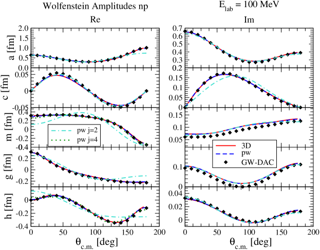
Figure 1: The Wolfenstein amplitudes for neutron-proton scattering at 100 MeV laboratory kinetic energy based on the AV18 potential. The solid (red) line represents the 3D calculation, whereas the dashed (blue) curve is obtained from a partial-wave calculation summing partial waves up to $j=6$. The partial-wave sums up to $j=2$ and $j=4$ are shown as double-dash-dotted (turquoise) and dotted (green) lines. The data points are the amplitudes extracted from the GW-DAC current analysis http://gwdac.phys.gwu.edu ; Arndt et al. (2007).

In this subsection we calculate the Wolfenstein amplitudes for neutron-proton ($np$) and proton-proton ($pp$) scattering calculated with our 3D formulation at 100 MeV and at 350 MeV laboratory energy and compare them with calculations Weppner et al. (1998) based on summing partial wave amplitudes up to a given $j_{max}$. We chose 100 MeV as the low energy, since here already the sum over a small number of partial waves should suffice to achieve agreement with the 3D calculation. This is indeed the case as illustrated in Fig. 1 for the $np$ Wolfenstein amplitudes. The solid line represents the 3D calculations, which perfectly agrees with a partial-wave calculation in which $j_{max}=6$. The figure also indicates that at this energy even $j_{max}=4$ already converges to the 3D result. We also compare our calculations to an extraction of the $np$ Wolfenstein amplitudes from the current solution of the GW-DAC Data Analysis Center Arndt et al. (2007, 2009); http://gwdac.phys.gwu.edu .

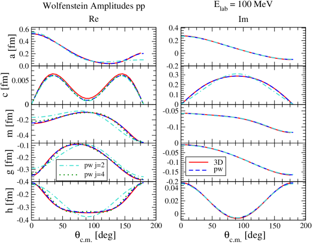
Figure 2: The Wolfenstein amplitudes for proton-proton scattering a 100 MeV laboratory kinetic energy based on the AV18 potential. The meaning of the curves is the same as in Fig. 1.

In Fig. 2 the Wolfenstein amplitudes for $pp$ scattering are shown for 100 MeV laboratory scattering energy, and again the 3D calculation is compared to a partial wave sum up to $j_{max}=6$. Here $pp$ means that we use the strong $pp$ interaction as given by the AV18 interaction, however do not treat the long-range Coulomb interaction. The 3D and partial-wave summed calculation agree rather well with each other. Only the Real $c$ amplitude displays a small deviation. However, when considering the scale of the y-axis, this deviation should not be considered significant. In contrast to the $np$ case, the real part of the amplitudes $g$ and $h$ indicate that for very small angles a $j_{max}=4$ calculation is not yet fully converged.

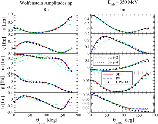
Figure 3: The Wolfenstein amplitudes for neutron-proton scattering at 350 MeV laboratory kinetic energy based on the AV18 potential.The solid (red) line represents the 3D calculation, whereas the dashed (blue) curve is obtained from a partial-wave calculation summing partial waves up to $j=9$. The partial-wave sums up to $j=2$ and $j=4$ are shown as double-dash-dotted (turquoise) and dotted (green) lines. The data points are the amplitudes extracted from the GW-DAC current analysis http://gwdac.phys.gwu.edu ; Arndt et al. (2007).

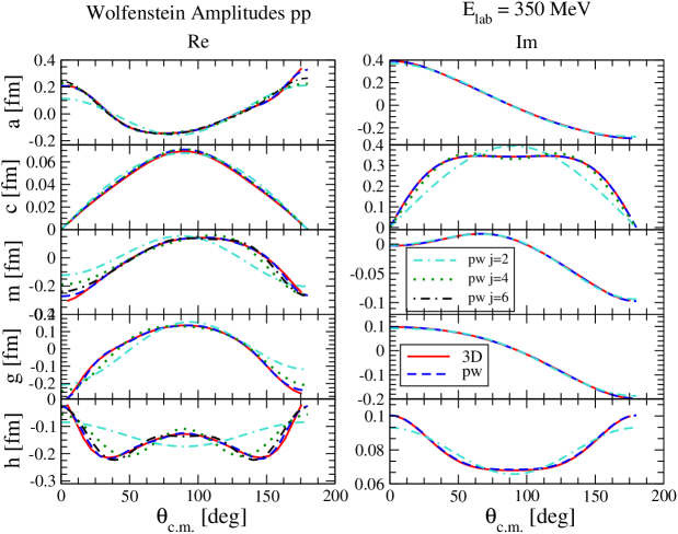
Figure 4: The Wolfenstein amplitudes for proton-proton scattering at 350 MeV laboratory kinetic energy based on the AV18 potential. The meaning of the curves is the same as in Fig. 3.

Figs. 3 and 4 show the Wolfenstein amplitudes for $np$ and $pp$ scattering at 350 MeV laboratory kinetic energy, the highest energy for which the AV18 interaction is fitted to the NN data base. In both figures the solid line represents the 3D calculation, whereas the dashed line represents a partial-wave calculation summed up to $j_{max}=9$. In Fig. 3 the partial-wave sums up to $j_{max}=2$ and $j_{max}=4$ are also shown. In contrast to the lower energy of 100 MeV in Fig. 1, at this energy the partial-wave sum up to $j_{max}=4$ is clearly not converged. In fact, the backward angles of the real parts of $a$ and $h$ show a particularly bad convergence. In addition, we indicate the extraction of the Wolfenstein amplitudes from the GW-DAC data analysis Arndt et al. (2007); http://gwdac.phys.gwu.edu by the filled diamonds. For the $pp$ Wolfenstein amplitudes in Fig. 4 we also display a partial wave calculation summed up to $j_{max}=6$ to indicate that even this partial wave sum is not yet converged to the full 3D calculation. A careful inspection of the real parts of the forward and backward angles of $a$, $g$, and $h$ reveals that even the partial wave sum of $j_{max}=9$ is not quite converged yet. In contrast, the imaginary parts of all amplitudes show already convergence at roughly $j_{max}=4$.

IV.3 Numerical Details

The LS integral equation that needs to be solved when performing a calculation without employing a partial-wave decomposition is, in the form of Eqs. (42) and (45), a two-dimensional integral equation in two variables (the magnitude of a momentum p’ and an angle x’). Due to the structure of the equation, an angle integration over the azimuthal angle $\phi$ can be carried out separately as given in Eq. (39), and is thus not part of the integral equation. For the integration we use standard Gauss-Legendre integration with a tangent map of the points of the momentum integration. Discretized the set of coupled equations, Eqs. (42) and (45), turn into a finite set of linear algebraic equations, which is solved by standard methods.

However, we need to test the numerical convergence for each integration. In the following we demonstrate the numerical convergence by concentrating on the real part of the Wolfenstein $a$ amplitude and consider its values for different sets of grid points of $p$, $x\equiv\cos\theta$, and $\phi$. For the choice of $n$ $p$-points, $m$ $x$-points and $l$ $\phi$-points let us define the value of the real part of the Wolfenstein amplitude A as $a(n,m,l)$. Then we define as logarithmic error in $\phi$,

$${\rm Log-Error}_{\phi}(l)=\log\left(\left|\frac{(a(60,30,40)-a(60,30,l))*100}{a(60,30,40)}\right|\right)$$ (105)

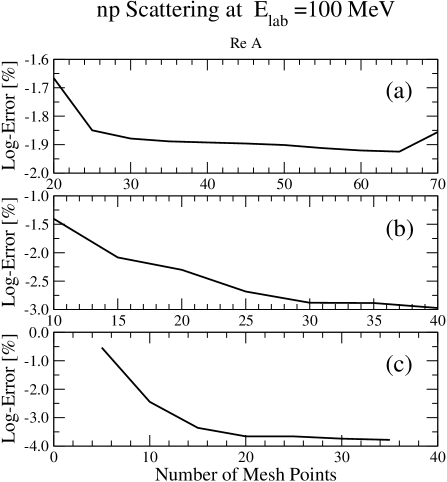
Figure 5: The logarithmic error for the momentum grid points (a), the polar angle ($\cos\theta=x$) points (b) and the azimuthal angle ($\phi$) grid points (c) as function of number of points. Precise definitions and explanations are given in Sec. IV.3.

This Log-Error is plotted in Fig. 5(c) for values $l\in(5,35)$, and we see that the $\phi$ integration converges very quickly. Already 20 $\phi$ points are sufficient to achieve an error in the order of $10^{-4}$%. For most of our calculations we choose 30 $\phi$ points. For the $x$-points we define

$${\rm Log-Error}_{x}(m)=\log\left(\left|\frac{(a(60,45,20)-a(60,m,20))*100}{a(60,45,20)}\right|\right)$$ (106)

This Log-Error is plotted in Fig. 5(b) for values $m\in(10,40)$. The $x$-integration converges much slower with respect to the number of mesh-points, and for having an error in the order of $10^{-3}$to $10^{-4}$% we need at least 40 integration points for a converged calculation.

For the momentum-integration points we define

$${\rm Log-Error}_{p}(n)=\log\left(\left|\frac{(a(75,30,20)-a(n,30,20))*100}{a(75,30,20)}\right|\right)$$ (107)

This Log-Error is plotted in Fig. 5(a) for values $n\in(20,70)$. Here we see that the error in the momentum integration decreases slowest as a function of the momentum-integration points, and in order to have an error of about $10^{-2}$% and we choose 60 $p$-points for our calculations. Based on the above considerations, all of our calculations use $(n,l,m)=(30,40,60)$ mesh points to achieve an overall numerical errors of 0.01%, which is well below the accuracy with which NN observables are given.

V Observables

One of the main purposes of this paper it to test the momentum-space potential AV18 potential given in Veerasamy and Polyzou (2011). There it was demonstrated that the potential reproduced the deuteron binding energy and the wave functions. However, these tests were only sensitive to the $np$ part of the potential. Now we have the opportunity to test the $np$ as well as the $pp$ pieces of the AV18 potential given in Ref. Veerasamy and Polyzou (2011). In comparing the results of the scattering calculations to data we found that the grid for the Fourier transform of the charge symmetry breaking term, which is the 18-th operator in Ref. Wiringa et al. (1995) needed to be extended beyond 100 fm^-1, the standard value for all other terms of the AV18 potential. Specifically, for the 18th operator the Chebyshev expansion of the Fourier transform is extended to 250 fm^-1.

The scattering amplitude matrix is related to the on-shell solution of the Lippmann-Schwinger equation as indicated in Eq. (72). Having obtained $M({\bf p}^{\prime},{\bf p})$, the spin averaged unpolarized differential cross section is given by summing over the final spins and averaging over the initial spins as

$${d\sigma\over d\Omega}=\frac{1}{4}\mathbf{Tr}(MM^{\dagger}),$$ (108)

whereas general spin observables have the form

$$\langle O\rangle=\frac{\mathbf{Tr}(MAM^{\dagger}B)}{\mathbf{Tr}(MM^{\dagger})}.$$ (109)

Here the operator $A$ is associated with a measurement of the initial spins and the operator $B$ is associated with a measurement of the final spin state. The traces can be expressed as homogeneous polynomials of degree two in terms of the Wolfenstein parameters.

To test the potential and the computational method we compare calculated $np$ observable as several energies and compare them to the observables in the GW-DAC analysis Arndt et al. (2007); http://gwdac.phys.gwu.edu as well as calculations based on a partial-wave expansion Weppner et al. (1998). For the $pp$ observables we can only make a comparison with the partial-wave based calculations, since we do not include the Coulomb interaction.

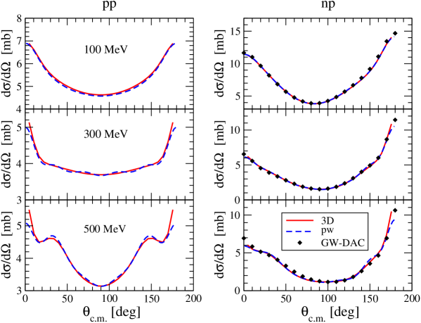
Figure 6: The differential cross section for $pp$ (left) and $np$ (right) scattering as function of the c.m. scattering angle for 100, 300, and 500 MeV projectile laboratory kinetic energy. The solid (red) line represent the 3D calculation with the AV18 potential, whereas the dashed line represent a partial-wave based calculation summed up to $j_{max}=9$. The diamonds represent the $np$ data from the GW-DAC analysis http://gwdac.phys.gwu.edu ; Arndt et al. (2007).

Fig. 6 shows the differential cross sections for $pp$ and $np$ scattering at 100, 300, and 500 MeV projectile laboratory kinetic energies. The solid lines are the result of solving the equations of Sec. III with the momentum-space AV18 potential of ref. Veerasamy and Polyzou (2011). Both calculations are compared to partial-wave calculations using a partial-wave sum up to $j_{max}=9$. The black diamonds are the $np$ cross sections taken from the GW-DAC phase shift analysis Arndt et al. (2007); http://gwdac.phys.gwu.edu . For the higher projectile laboratory kinetic energies there is a clear deviation at the very forward and backward angles between the 3D calculation and the partial-wave sum, indicating that even the sum to $j_{max}=9$ is not yet converged.

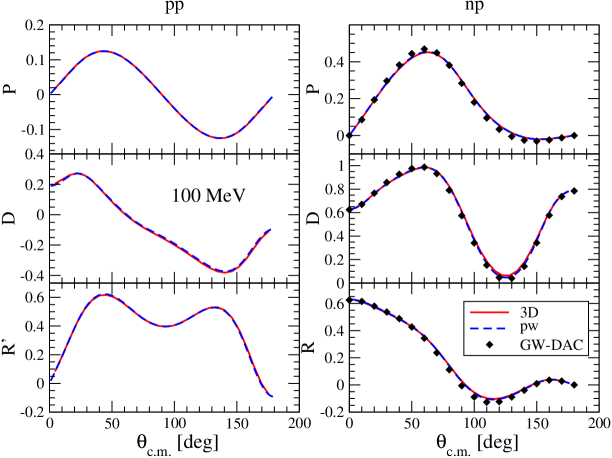
Figure 7: The spin observables $P$, $D$ and $R^{\prime}$ for $pp$ (left) and $np$ (right) scattering as function of the c.m. scattering angle for 100 MeV projectile laboratory kinetic energy. The solid (red) line represent the 3D calculation with the AV18 potential, whereas the dashed line represent a partial-wave based calculation summed up to $j_{max}=9$. The diamonds represent the $np$ data from the GW-DAC analysis http://gwdac.phys.gwu.edu ; Arndt et al. (2007).

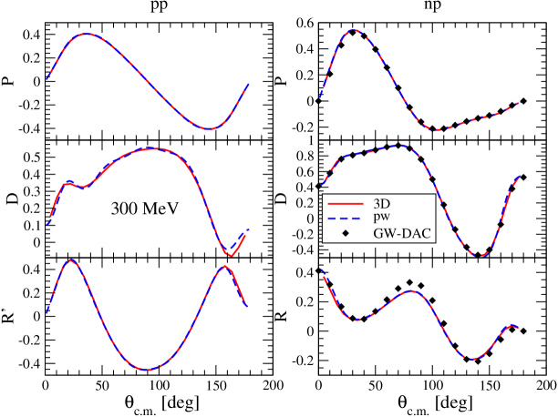
Figure 8: The spin observables $P$, $D$ and $R^{\prime}$ for $pp$ (left) and $np$ (right) scattering as function of the c.m. scattering angle for 300 MeV projectile laboratory kinetic energy. The meaning of the curves is the same as in Fig. 7.

Figs. 7 and 8 show selected spin observables for $pp$ and $np$ scattering at 100 and 300 MeV. The following observables are shown,

$$\mathbf{P} = \frac{\mathbf{Tr}(MM^{\dagger}\mbox{\boldmath$\sigma$})}{\mathbf{Tr}(MM^{\dagger})}$$ (110)

$$D = \frac{\mathbf{Tr}(M(\mbox{\boldmath$\sigma$}\cdot\hat{\mathbf{N}})M^{\dagger}(\mbox{\boldmath$\sigma$}\cdot\hat{\mathbf{N}))}}{\mathbf{Tr}(MM^{\dagger})}$$ (111)

$$R^{\prime} = \frac{\mathbf{Tr}(M(\mbox{\boldmath$\sigma$}\cdot(\hat{\mathbf{N}}\times\mathbf{Q}))M^{\dagger}(\mbox{\boldmath$\sigma$}\cdot\hat{\mathbf{Q}}))}{\mathbf{Tr}(MM^{\dagger})}.$$ (112)

Here $\sigma$ stands for either $\mbox{\boldmath$\sigma$}_{1}$ or $\mbox{\boldmath$\sigma$}_{2}$ depending on label of the particles. The solid lines represent the 3D calculation with the the momentum-space AV18 potential of ref. Veerasamy and Polyzou (2011), whereas the dashed lines represent a partial-wave calculation with partial waves summed up to $j_{max}=9$. The diamonds represent the observables taken from the GW-DAC analysis Arndt et al. (2007); http://gwdac.phys.gwu.edu . At 100 MeV projectile kinetic energy there is perfect agreement between the 3D and the partial-wave calculations, as is expected. At 300 MeV there are small deviations in the backward angles of $D$ and $R^{\prime}$, however not as large as for the differential cross section.

VI Summary and Conclusions

We formulated and numerically illustrated an approach to treat NN scattering directly with momentum vectors together with spin-momentum operators multiplied with scalar function that are only functions of those momentum vectors. Our formulation differs from the one suggested previously in Ref. Golak et al. (2010) in the choice of the operator expansion. The basic foundation for an operator expansion rests on the fact that the most general form of a nucleon-nucleon interaction can be represented as a linear combination of six linearly independent spin-momentum operators with scalar coefficient functions. The Wolfenstein decomposition of the NN scattering amplitude into five linearly independent operators is dictated by physical symmetries Wolfenstein and Ashkin (1952), while a sixth operator with those symmetry properties does not exist on-shell. The choice of this sixth operator is not unique, and different NN potential employ different choices Fachruddin et al. (2000); Crespo and Moro (2002).

In this work we solve the Lippmann Schwinger equation by using different numbers of spin-momentum basis elements to represent the on- and half-off shell transition matrix elements. We show that a numerically stable discretization of the Lippmann-Schwinger equation is obtained for a certain pair of on and off-shell spin bases. The stable choice includes a sixth time-odd operator in the off-shell basis. The choice of this sixth operator is the main difference between our formulation and calculation compared to the ones in Ref. Golak et al. (2010). Our calculations are able to directly calculate the on-shell elements of the transition amplitude, which was not easily possible with the choice of Ref. Golak et al. (2010). We should point out that even if a time-odd operator appears in the expansion of the potential, as it does in the AV18 potential, the potential itself remains invariant with respect to time reversal, since the expansion coefficients of this operator also contain time-odd functions. The scalar coefficient function time-odd operator we consider vanishes on shell.

With those six operators the Lippmann-Schwinger equation becomes a six channel integral equation in two variables. The solution is represented by six complex amplitudes in four variables, which on-shell reduce to five complex amplitudes in two variables, which are simple linear combinations of the five Wolfenstein amplitudes. We calculated the Wolfenstein amplitudes for $np$ and $pp$ scattering using the momentum-space representation of the AV18 potential given in Ref. Veerasamy and Polyzou (2011) for several laboratory projectile kinetic energies and compared our calculations to the results of traditional partial-wave calculations summed up to a given $j_{max}$ and verified for low energies that our 3D calculation matches the partial-wave sum exactly, while at even moderately high energies (like e.g. 300 MeV) a partial-wave sum with $j_{max}\leq 9$ is not sufficient for a converged partial-wave calculation.

Appendix A Transition Matrix Elements

In order to keep the notation as simple as possible we use shorthand notations for the terms in Eqs. (48-51):

$$t_{il} := t(p_{i}^{\prime\prime},p_{0},x^{\prime\prime}_{l};p_{0})$$ (113)

$$t_{0l} := t(p_{0},p_{0},x^{\prime}_{l};p_{0})$$ (114)

$$v_{il} := v(p_{i}^{\prime},p,x^{\prime}_{l})$$ (115)

$$v_{0l} := v(p_{0},p,x^{\prime}_{l})$$ (116)

$$u_{il;jk} := u(p_{i}^{\prime},x^{\prime}_{l},p_{j}^{\prime\prime},x_{k}^{\prime\prime})$$ (117)

$$u_{il;0k} := u(p_{i}^{\prime},x^{\prime}_{l},p_{0},x_{k}^{\prime\prime})$$ (118)

$$u_{0l;jk} := u(p_{0},x^{\prime}_{l},p_{j}^{\prime\prime},x_{k}^{\prime\prime})$$ (119)

$$u_{0l;0k} := u(p_{0},x^{\prime}_{l},p_{0},x_{k}^{\prime\prime})$$ (120)

$$g_{j} := {2\mu\over p_{0}^{2}-p_{j}^{\prime\prime 2}+i0^{+}}.$$ (121)

In this notation Eqs. (48-51) become the linear system,

$$t_{il} = v_{il}+\sum_{kj}dx^{\prime\prime}_{k}dp^{\prime\prime}_{j}g_{j}[u_{il;jk}(p^{\prime\prime}_{j})^{2}t_{jk}-u_{il;0k}p_{0}^{2}t_{0k}]-{i2\pi\mu p_{0}}\sum_{k}dx^{\prime\prime}_{k}u_{il;0k}t_{0k}$$ (122)

$$t_{0l} = v_{0l}+\sum_{kj}dx^{\prime\prime}_{k}dp^{\prime\prime}_{j}g_{j}[u_{0l;jk}(p^{\prime\prime}_{j})^{2}t_{jk}-u_{0l;0k}p_{0}^{2}t_{0k}]-i2\pi\mu p_{0}\sum_{k}dx^{\prime\prime}_{k}u_{0l;0k}t_{0k}.$$ (123)

The interaction and transition matrix elements are represented by linear combinations of the operators, $W^{j}$. Since the $W^{j}$ operators depend on the momenta, there are different expansions at each quadrature point. We use the notation $\hat{W}^{j}$ for the operators used to expand the on-shell matrix elements and $W^{j}$ for the operators used to expand the off-shell matrix elements, even though they are identical for $j=1,\cdots,5$. Lower indices are used to denote the momentum variables that appear in the operator expressions.

$$t_{il} := \sum_{m=1}^{6}t_{il}^{m}W_{il}^{m}$$ (124)

$$t_{0l} := \sum_{m=1}^{5}t_{0l}^{m}\hat{W}_{l}^{m}$$ (125)

$$v_{il} := \sum_{m=1}^{6}v_{il}^{m}W_{il}^{m}$$ (126)

$$v_{0l} := \sum_{m=1}^{5}v_{0l}^{m}\hat{W}_{l}^{m}$$ (127)

$$u_{il;jk} := \sum_{m=1}^{6}u_{iljk}^{m}W_{iljk}^{m}$$ (128)

$$u_{il;0k} := \sum_{m=1}^{6}u_{il0k}^{m}{W}_{ilk}^{m}$$ (129)

$$u_{0l;jk} := \sum_{m=1}^{6}u_{0l0k}^{m}{W}_{ilk}^{m}$$ (130)

$$u_{0l;0k} := \sum_{m=1}^{5}u_{lk}^{m}\hat{W}_{lk}^{m}.$$ (131)

Substituting these expansions into Eqs. (123) leads to

$$\sum_{m=1}^{6}t_{il}^{m}W_{il}^{m}=\sum_{m=1}^{6}v_{il}W_{il}^{m}+$$ (134)

$$\sum_{kj}dx_{k}^{\prime\prime}dp_{j}^{\prime\prime}g_{j}\left[\sum_{m,n=1}^{6}u^{m}_{iljk}(p_{j}^{\prime\prime 2})t^{n}_{jk}W_{iljk}^{m}W_{jk}^{n}-\sum_{m=1}^{6}\sum_{n=1}^{5}u^{m}_{il0k}p_{0}^{2}t^{n}_{0k}{W}_{ilk}^{m}\hat{W}_{k}^{n}\right]$$

$$-{i2\pi\mu p_{0}}\sum_{k}dx_{k}^{\prime\prime}\sum_{m=1}^{6}\sum_{n=1}^{5}u^{m}_{il0k}t^{n}_{0k}{W}_{ilk}^{m}\hat{W}_{k}^{n}$$

and

$$\sum_{m=1}^{5}t^{m}_{0l}\hat{W}_{l}^{m}=\sum_{m=1}^{5}v^{m}_{0l}\hat{W}_{l}^{m}+$$ (137)

$$\sum_{kj}dx_{k}^{\prime\prime}dp_{j}^{\prime\prime}g_{j}\left[\sum_{m,n=1}^{6}u^{m}_{0ljk}(p_{j}^{\prime\prime 2})t^{n}_{jk}W_{ljk}^{m}W_{jk}^{n}-\sum_{m=1}^{6}\sum_{n=1}^{5}u^{m}_{0l0k}p_{0}^{2}t^{n}_{0k}{W}_{lk}^{m}\hat{W}_{k}^{n}\right]$$

$$-i2\pi\mu p_{0}\sum_{k}dx_{k}^{\prime\prime}\sum_{m,n=1}^{5}u^{m}_{0l0k}t^{n}_{0k}\hat{W}_{lk}^{m}\hat{W}_{k}^{n}$$

In order to obtain a linear system for the coefficient functions, $t^{m}_{il}$ and $t^{m}_{0l}$, we first multiply the first equation from the left by $W_{il}^{m^{\prime}}$ and the second one by $\hat{W}_{l}^{m^{\prime}}$ and then take traces over the spins. The resulting linear system is given by

$$\sum_{m=1}^{6}t_{il}^{m}\mbox{Tr}(W_{il}^{m^{\prime}}W_{il}^{m})=\sum_{m=1}^{6}v_{il}\mbox{Tr}(W_{il}^{m^{\prime}}W_{il}^{m})+$$ (140)

$$\sum_{kj}dx_{k}^{\prime\prime}dp_{j}^{\prime\prime}g_{j}\left[\sum_{m,n=1}^{6}u^{m}_{iljk}(p_{j}^{\prime\prime 2})t^{n}_{jk}\mbox{Tr}(W_{il}^{m^{\prime}}W_{iljk}^{m}W_{jk}^{n})-\sum_{m=1}^{6}\sum_{n=1}^{5}u^{m}_{il0k}p_{0}^{2}t^{n}_{0k}\mbox{Tr}(W_{il}^{m^{\prime}}{W}_{ilk}^{m}\hat{W}_{k}^{n})\right]$$

$$-{i2\pi\mu p_{0}}\sum_{k}dx_{k}^{\prime\prime}\sum_{m=1}^{6}\sum_{n=1}^{5}u^{m}_{il0k}t^{n}_{0k}\mbox{Tr}(W_{il}^{m^{\prime}}{W}_{ilk}^{m}\hat{W}_{k}^{n})$$

and

$$\sum_{m=1}^{5}t^{m}_{0l}\mbox{Tr}(\hat{W}_{l}^{m^{\prime}}\hat{W}_{l}^{m})=\sum_{m=1}^{5}v^{m}_{0l}\mbox{Tr}(\hat{W}_{l}^{m^{\prime}}\hat{W}_{l}^{m})+$$ (143)

$$\sum_{kj}dx_{k}^{\prime\prime}dp_{j}^{\prime\prime}g_{j}\left[\sum_{m,n=1}^{6}u^{m}_{0ljk}(p_{j}^{\prime\prime 2})t^{n}_{jk}\mbox{Tr}(\hat{W}_{l}^{m^{\prime}}W_{ljk}^{m}W_{jk}^{n})-\sum_{m=1}^{6}\sum_{n=1}^{5}u^{m}_{0l0k}p_{0}^{2}t^{n}_{0k}\mbox{Tr}(\hat{W}_{l}^{m^{\prime}}{W}_{lk}^{m}\hat{W}_{k}^{n})\right]$$

$$-i2\pi\mu p_{0}\sum_{k}dx_{k}^{\prime\prime}\sum_{m,n=1}^{5}u^{m}_{0l0k}t^{n}_{0k}\mbox{Tr}(\hat{W}_{l}^{m^{\prime}}\hat{W}_{lk}^{m}\hat{W}_{k}^{n}).$$

The input to Eqs. (140) through (143) involves a large number of traces over the spin operators. To treat these we use the symbolic tool developed in Veerasamy (2011) to evaluate these traces.