Multiple Star Formation to the Bottom of the IMF

Abstract

The frequency and properties of multiple star systems offer powerful tests of star formation models. Multiplicity surveys over the past decade have shown that binary properties vary strongly with mass, but the functional forms and the interplay between frequency and semimajor axis remain largely unconstrained. We present the results of a large-scale survey of multiplicity at the bottom of the IMF in several nearby young associations, encompassing 78 very low mass members observed with Keck laser guide star adaptive optics. Our survey confirms the overall trend observed in the field for lower-mass binary systems to be less frequent and more compact, including a null detection for any substellar binary systems with separations wider than $\sim$7 AU. Combined with a Bayesian re-analysis of existing surveys, our results demonstrate that the binary frequency and binary separations decline smoothly between masses of 0.5 $M_{\sun}$ and 0.02 $M_{\sun}$, though we can not distinguish the functional form of this decline due to a degeneracy between the total binary frequency and the mean binary separation. We also show that the mass ratio distribution becomes progressively more concentrated at $q\sim$1 for declining masses, though a small number of systems appear to have unusually wide separations and low mass ratios for their mass. Finally, we compare our results to synthetic binary populations generated by smoothed particle hydrodynamic simulations, noting the similarities and discussing possible explanations for the differences.

1. Introduction

The frequency and properties of multiple star systems offer powerful constraints on star formation and early cluster evolution. The semimajor axis of a binary system should correspond to the characteristic size of its progenitor core at the time of fragmentation, so the binary separation distribution constrains the range of sizes and the size evolution for cores(e.g., Sterzik et al., 2003, and references therein). The overall binary frequency and the mass ratio distribution are set by the detailed physics of binary fragmentation(Delgado-Donate et al., 2004), and each binary system’s mass ratio will depend on the post-fragmentation accretion history(Bate & Bonnell, 1997), while formation in environments with high stellar density could shape the binary population as and after it forms(Kroupa et al., 1999). A successful model for star formation should be able to match the observed frequency and properties of the binary star population, as well as any mass-dependent changes in these parameters.

The past two decades have seen numerous studies of nearby field binary systems in order to constrain their frequency and properties. These surveys (e.g., Duquennoy & Mayor, 1991; Fischer & Marcy, 1992; Close et al., 2003; Bouy et al., 2003; Burgasser et al., 2003) have found that binary frequencies and properties are very strongly dependent on mass. Solar-mass stars have high binary frequencies ($\gtrsim$60%) and maximum separations of up to $\sim$10⁴ AU. By contrast, M dwarfs have moderately high binary frequencies (30–40%) and few binary companions with separations of more than $\sim$1000 AU, while brown dwarfs have low binary frequencies ($\sim$15% for all companions with separations $\gtrsim$2–4 AU) and few companions with separations $>$10 AU.

However, field multiplicity results face unavoidable ambiguity near and below the substellar regime. These surveys provide only weak constraints on the mass dependence of substellar binary properties due to the degeneracy between brown dwarf masses and ages, and mass ratios are similarly difficult to estimate. Also, the field represents a composite population drawn from all star-formation regions, so field surveys cannot probe the dependence of binary properties on initial conditions (the stellar density or total mass) and evolutionary history (the degree of dynamical evolution each system undergoes before leaving its natal environment). For example, the separation distribution for binary systems is truncated at separations of $\sim$100 AU in open clusters like Praesepe (e.g., Patience et al., 2002), whereas unbound young associations have binary systems as wide as 10⁴ AU (Kraus & Hillenbrand, 2008, 2009b).

These complications have motivated a large number of multiplicity surveys in nearby star-forming regions and young clusters. Several survey programs have found that the solar-mass stars in loosely-bound young associations have extremely high binary frequencies(Ghez et al., 1993; Leinert et al., 1993; Simon et al., 1995; Köhler et al., 2000; Kraus et al., 2008). The binary frequency in young open clusters appears to be significantly lower(e.g., Petr et al., 1998; Köhler et al., 2006), which could be interpreted either as early dynamical evolution or a signature of the different primordial environment. Surveys of very low-mass stars and brown dwarfs have concentrated mainly on nearby unbound associations (Kraus et al., 2005, 2006; Konopacky et al., 2007; Ahmic et al., 2007; Biller et al., 2011), but produced results that largely match the field: low-mass binary systems are rare and tend to have small separations and similar component masses.

The aforementioned surveys of low-mass multiplicity in young associations used very modest sample sizes since high-resolution imaging techniques were observationally expensive. As a result, their tentative conclusions raised as many questions as they answered. The handful of binary systems they discovered tended to fall in the upper end of the surveys’ mass ranges, with very few binary companions to genuinely substellar primaries. This suggested that the binary frequency might decline with primary mass through this range, an observation that is difficult to test among low-mass field binaries.

The limited sample sizes and heterogeneous nature of previous surveys have prohibited any detailed analysis of the mass dependence of multiple star formation, especially in the low-mass regime ($M\lesssim$0.15 $M_{\sun}$) where mass-dependent effects seem to be most significant. To address this shortcoming, we present a large-scale survey of multiplicity at the bottom of the IMF in several nearby young associations. In Section 2, we list our survey’s sample and describe our survey’s observations, and in Section 3, we explain the analysis techniques used in our program. In Section 4, we describe the results of our observations. Finally, in Section 5, we use our results and other results from the literature to constrain the mass-dependent properties of low-mass multiple star formation and compare those properties to the results of theoretical models.

2. Sample and Observations

2.1. Sample Selection

Nearby star-forming regions have been the target of numerous wide-field photometric imaging surveys to detect new low-mass members (e.g., Luhman, 2004, 2006; Slesnick et al., 2006a, b, 2008). These surveys identified candidate members based on their location on an optical or near-infrared color-magnitude diagram, and membership was then confirmed spectroscopically via the detection of lithium absorption, excess $H\alpha$ emission, or low surface gravity, all of which are indicators of youth. We chose to concentrate on Taurus-Auriga ($\tau\sim$1–2 Myr; $d\sim 145$ pc; Kraus & Hillenbrand, 2009a; Torres et al., 2009) and Upper Scorpius ($\tau\sim$5 Myr; $d\sim 145$ pc; de Zeeuw et al., 1999; Preibisch et al., 2002)because they are the nearest young associations that are accessible from the northern hemisphere. In our analysis, we also use results from the literature on the Cha-I association ($\tau\sim$2–3 Myr; $d\sim 185$ pc; Luhman, 2004), which is similar to Taurus in age and environment. All regions have very low stellar densities ($N\lesssim$10 pc^-3), which is critical for minimizing the complicating role of dynamical interactions.

Our initial observational sample included all late-type members of each association (SpT$\geq$M4) that had been identified by 2006 and that hadn’t been observed at high angular resolution. However, as we describe in Section 3, we lost a significant fraction of our observing time to poor weather and instrument problems. This left our Taurus sample significantly incomplete for members discovered in 2006, plus we were unable to observe three members that had been identified earlier (J1-4423, V410 X-ray 6, and 2MASS J04163049). The effect on Upper Sco was to limit our observed sample to only the latest-type members (SpT$\geq$M6.5). We also were unable to observe 10 Taurus members that had no suitable tip-tilt stars available. This omission introduces a bias against the most reddened members of Taurus since the most heavily extincted stars were least likely to have an optically bright star nearby that could serve as a tip-tilt reference. The density of field stars is very high in Upper Sco, plus the association is almost completely cleared of its primordial molecular material, so we were always able to find a suitable tip-tilt star.

We have supplemented this observational sample with the results of numerous previous multiplicity surveys. Taurus has been a very popular target for multiplicity surveys, and association members in our spectral type range have been observed with speckle interferometry (Ghez et al., 1993; Konopacky et al., 2007), lunar occultations (Simon et al., 1995), HST imaging (Padgett et al., 1999; White & Ghez, 2001; Kraus et al., 2006), AO imaging (Correia et al., 2006), and aperture-masking interferometry (Kraus et al., 2011). Upper Scorpius has been the subject of several surveys as well, and members have been observed with speckle interferometry (Köhler et al., 2000), HST imaging (Kraus et al., 2005), and AO imaging and aperture-masking interferometry (Kraus et al. 2008). In most cases (and almost certainly in aggregate), the sample members were selected seemingly at random. As a result, we adopt the combined set as an unbiased sample.

Finally, we also observed a small number of other targets that fall outside these selection parameters, but were considered interesting for other reasons. In both associations, we observed a number of candidate wide binary systems that seemed to have unusually low binding energies. We already described the observations for UScoJ1606-1935 in a previous paper (Kraus & Hillenbrand, 2007c), and we reported the astrometric measurements for the rest in our paper on wide binary formation (Kraus & Hillenbrand, 2009b). In this paper, we report on the search for higher-order multiplicity. We also observed several candidate Taurus members discovered by (Slesnick et al., 2006b) that are not part of the young Taurus population, but might represent an older, more widely distributed population of young stars and brown dwarfs. Finally, we observed the known binary V928 Tau because it served as the tip-tilt reference for CFHT-Tau-7 and we typically imaged tip-tilt references for a data quality check. However, we do not report any results for CFHT-Tau-7 because the observing conditions at the time were too marginal for adaptive optics to yield any meaningful correction.

In Table 1, we list the young association members that we observed in our study. The $K$ magnitude for each target was taken from 2MASS (Skrutskie et al. 2006), while the $R$ magnitude and distance to each star’s tip-tilt reference are from the USNO-B1.0 catalog (Monet et al. 2003). We also list references for the handful of objects which have also been observed in other high-resolution imaging surveys; in several cases, our detection limits for small separations were superceded by the survey by Konopacky et al. (2007), so we adopted those limits where appropriate.

2.2. Observations

Most of the data that we summarize were obtained in 4 observing runs, totaling 10 nights, between December 2005 and March 2007. One source was observed during a time trade in December 2006. Most of our observations were obtained using laser guide star adaptive optics (LGSAO; Wizinowich et al., 2006) on the Keck-II telescope with NIRC2 (K. Matthews, in prep), a high spatial resolution near-infrared camera. During some periods of moderate cloud cover that were not suitable for laser operation, we also used natural guide star adaptive optics (NGSAO) to observe sample members with very close and bright tip-tilt stars. In the worst conditions, we also observed some higher-mass stars that did not fall in our sample; most of these observations have been described in our previous papers (Kraus & Hillenbrand, 2008, 2009b), so we report the rest here for completeness.

The weather conditions were highly variable over the course of our campaign, with only five nights suitable for laser operations. Several of the remaining nights were also impacted by poor seeing. Despite numerous difficulties, we report 82 observations of young association members with LGSAO and 5 additional observations with NGSAO, encompassing 78 different targets. In Table 2, we summarize the observations for each target. We also list the typical PSF FWHM for each target; a significant fraction of the targets used bright on-axis tip-tilt stars that should have achieved diffraction-limited performance (strehl$\sim$30%), but we only achieved this performance on two nights.

All of the images presented here were produced with the narrow camera, which has a field of view of 10.2″and a pixel size of 9.963 mas pix^-1 (Ghez et al., 2008). All targets were observed with the $K_{p}$ filter; in most cases, we did not obtain observations in other filters because most background stars have $J-K$ and $H-K$ colors that are not sufficiently different from young stars as to allow secure identification. Many results we draw from the literature appear to have been observed with $K$ or $K_{s}$ filters (though some do not specify), but we treat all three filters equivalently since the color terms are smaller than the typical photometric uncertainties (e.g., Carpenter et al. 2002). During early observing runs, we used a three-point dither pattern that was designed to avoid the bottom-left quadrant, which suffers from high read noise. After February 2006, we obtained all of our observations in a diagonal two-point dither pattern because experience showed that dithers degrade the AO correction until several exposures have been taken with the Low-Bandwidth Wavefront Sensor. The delay before returning to optimal correction represented a significant overhead that we sought to minimize.

Many of the targets are relatively bright in the NIR and require very short integration times to avoid saturation or nonlinearity, so a large fraction of our observations were taken in correlated double-sampling (CDS) mode, for which the array read noise is 38 electrons read^-1. Where possible, we observed targets in multiple correlated double-sampling (MCDS) mode, where multiple reads are taken at the beginning and ending of each exposure; this choice reduces the read noise by approximately the square root of the number of reads. This is doubly significant because the read noise per coadd and the total number of coadds per exposure are both reduced. In all cases, the read noise is negligible compared to PSF variations from the primary at separations of $<$1″. However, it always dominated over the sky background in determining our faint-source detection limits at large separations from the science target. In all cases, the images were flat-fielded and dark- and bias-subtracted using standard IRAF procedures.

3. Analysis Methods

3.1. Source Identification and Detection Limits

Source identification in AO imagery is a complicated endeavour. In NGSAO mode, the gross shape of the PSF depends on the target’s optical brightness and the seeing, while the fine structure is determined by speckle patterns that continuously change on timescales ranging from seconds to hours. The LGSAO PSF is further complicated by variations in laser return strength, tip-tilt anisoplanatism with respect to off-axis guide stars, and heightened sensitivity to telescope effects like wind shake. Finally, observations in poor weather are further complicated by rapid PSF quality variation due to changing atmospheric conditions. The source detection process can be divided into two regimes: a wide regime where the PSF core is negligible and speckle confusion dominates (projected separation $\rho$$\gtrsim$2 times the core FWHM), and a close regime where shape and width variations in the PSF core dominate and speckle confusion is negligible. We have adopted a different method in each separation regime.

3.1.1 The Wide, Speckle-Dominated Regime

As was summarized by Metchev & Hillenbrand (2009), there are four common methods used to subtract the primary star’s flux and identify companions in AO imagery: subtracting a median PSF representing all similar observations, subtracting a 180^o rotated version of the same image, high-pass filtering by subtracting a Gaussian-smoothed version of the same image, or subtracting the azimuthally-averaged profile. We conducted experiments with these techniques, but we found that the speckle mitigation strategies that are vital for high-strehl NGSAO data are actually only marginally useful for low-strehl LGSAO data. Most of the flux that would be found in discrete speckles in high-strehl data is instead averaged into the seeing-limited halo, rendering the PSF less azimuthally variable at a given separation. The brightest speckles remain distinguishable, but at far lower contrast with respect to the surrounding median flux. Since the noise floor is brighter and the noise ceiling is fainter, there is less to be gained from exceeding the noise ceiling.

The sparsity and relatively low contrast of speckles in LGSAO data suggest that a different strategy is optimal for our data. Speckle mitigation and subtraction of the primary star’s flux are observationally expensive, so the preferred strategy should be to characterize the mean and standard deviation of the brightness distribution of the PSF as a function of separation, then set the source detection limit above the expected ceiling for speckle brightness. We characterized the brightness distribution of each target’s PSF by measuring the flux through photometric apertures placed at a range of separations and PAs, then measuring the mean and standard deviation for all apertures in a given bin of separation. The apertures were placed on a rectangular grid with spacing of 25 mas in order to ensure that the small number of speckles were detected, and the aperture sizes were matched to the FWHM of the PSF core for the primary. We measured this aperture photometry using the IRAF task PHOT, which is distributed as part of the DAOPHOT package (Stetson, 1987).

In Figure 1, we show the contrast as a function of separation for three stars that span our survey’s data quality, as well as the 5$\sigma$ envelope for each source. We found that there was typically 1 detection at 4–5$\sigma$ per 2 stars, one detection at 5–6$\sigma$ per 10 stars, and no detections among any of our targets at 6–10$\sigma$. This indicates that a 6$\sigma$ clip should be uncontaminated by spurious detections, while a 5$\sigma$ clip can be adopted if the few remaining speckles can be confidently identified as such. We found that all of the 5–6$\sigma$ candidate detections fell on the PSF’s diffraction spikes, were sufficiently short-lived so as to not appear in all observations of a target, or were sufficiently long-lived so as to appear in observations of multiple sequential targets. We therefore suggest that all such 5–6$\sigma$ candidate detections are spurious, and adopt a 5$\sigma$ clip as our survey’s detection limits. All candidate detections that sit well above the 5$\sigma$ limit appear to be genuine astronomical sources, though not necessarily comoving companions; we will revisit this distinction in Section 5.2.

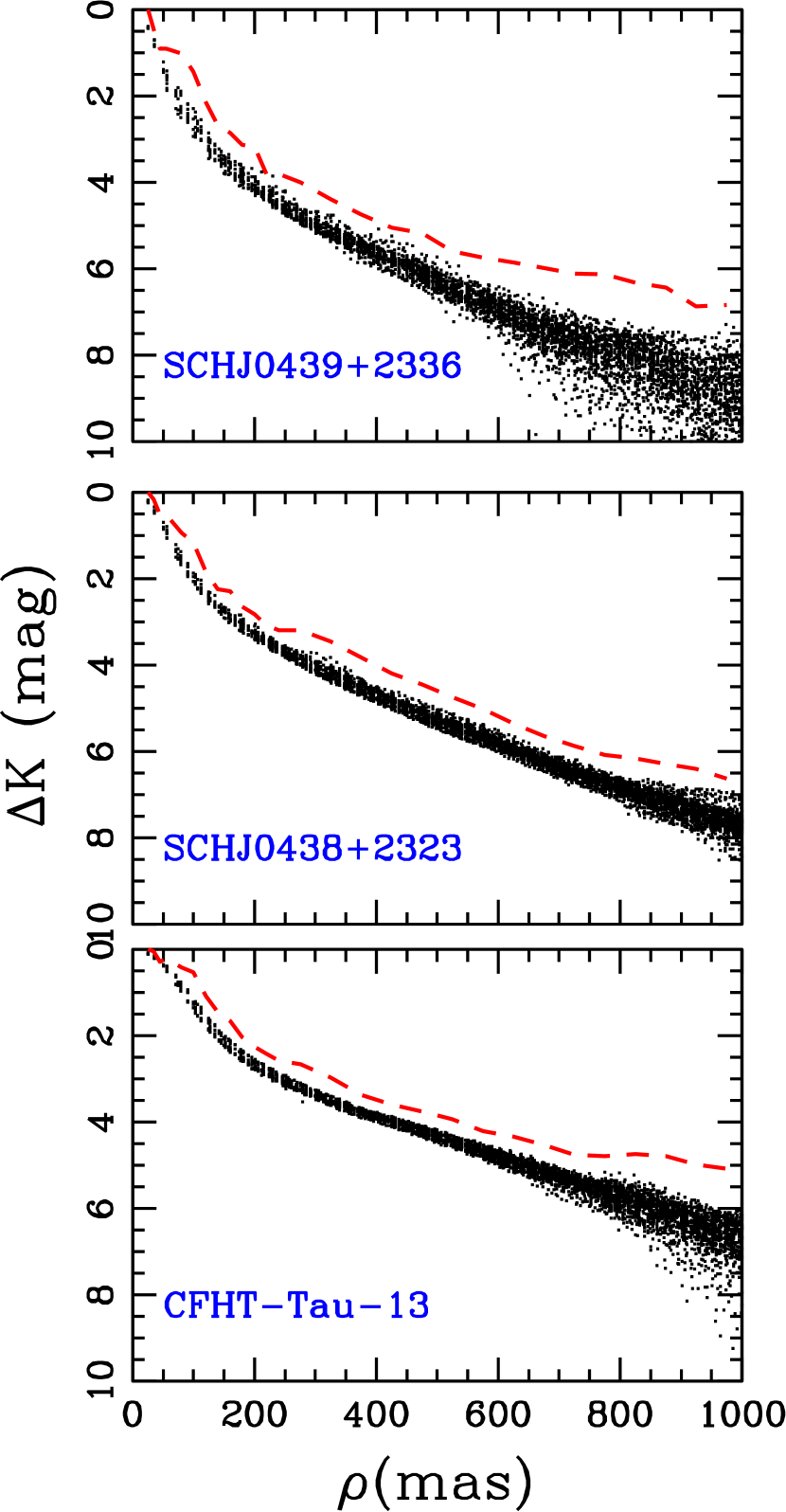
Figure 1.— Contrast limits at wide separations ($>$100 mas) for three representative stars in our sample: SCH J0439016+2336030 (top), SCH J0438587+2323596 (middle), and CFHT-Tau-13 (bottom). The small black points show the flux as a function of separation for apertures placed at a range of separations and PAs from the primary, while the red dashed line shows the +5 sigma envelope above these points. A handful of candidate sources fall above this significance level, but all can be identified as speckles, so we have defined this envelope for each target and use it as our survey’s detection limit. The main difference in contrast is determined by the quality of the tip-tilt reference star (Table 1); tip-tilt references which are brighter or located on-axis yield better AO correction.

3.1.2 The Close, Core-Dominated Regime

For separations near the PSF FWHM, the detection limits are driven by time- and spatially-dependent variations of the shape of the PSF core. LGSAO observations seem to be more susceptible to all of the weather effects that can degrade NGSAO observations, so distinguishing genuine companions from PSF artifacts is a significant challenge. The primary effect we see is for wind shake to cause PSF elongation in the direction of the zenith, perhaps because the tip-tilt sensor and low-bandwidth wavefront sensor operate at a lower rate and can’t fully sample high-frequency oscillations of the telescope. Tip-tilt anisoplanatism is also significant for observations with off-axis tip-tilt guide stars, an effect that becomes worse in poor seeing because the isokinetic angle becomes smaller. This causes elongation along the position angle to the tip-tilt star. Finally, significant variations in the AO correction cause the PSF FWHM itself to vary by a factor of $\sim$3 across our sample; a few of the lowest-quality observations have a PSF FWHM approaching 150 mas.

We have characterized these effects by fitting each science target’s PSF core with a bivariate Gaussian distribution. This fit directly yields the PSF elongation (the ratio of the major axis $a$ and minor axis $b$) and its direction (the PA of the major axis). For each our targets, we report the minor axis FWHM (i.e. the resolution prior to elongation effects) and the fractional elongation in Table 2. If windshake and tip-tilt anisoplanatism are the dominant sources of PSF asymmetry, then most sources should have a PA that is preferentially aligned with either the tip-tilt angle or the zenith angle. A set of selection criteria based on these quantities also lends itself to rigorous characterization of the detection limits, as artificial star tests can be used to determine whether a system with given separation and contrast (and perhaps PA) would be detected.

In Figure 2 (top), we plot the PSF elongation and the relative angle between the PSF and the zenith angle ($|\theta$_PSF-$\theta$${}_{zen}|$) for all science targets which served as their own tip-tilt references. Of the 21 sources which are not independently-confirmed binary systems, 9 are aligned to within $<$10^o of the zenith angle and 7 of the remaining 12 are aligned to within 10–45^o. This strong trend indicates that wind-induced elongation was significant across the majority of our sample, even on those nights with moderate winds. Also, all of the targets that are not independently-confirmed binary systems have elongations of $<$30%, which seems to be the ceiling for PSF elongation due to telescope or atmospheric effects.

In Figure 2 (bottom), we consider the rest of our sample in plotting the PSF elongation versus the minimum of the relative angle either between PSF and zenith ($|\theta$_PSF-$\theta$${}_{zen}|$) or between PSF and tip-tilt ($|\theta$_PSF-$\theta$${}_{TT}|$). These targets also show a pronounced tendency to align with either the zenith or tip-tilt, though the result is more complicated because many targets have a net elongation intermediate between the two directions. There are fewer confirmed binary systems for comparison, but most of the targets fall below elongations of 40%, suggesting that this is the ceiling for combined wind and tip-tilt effects. Many of the targets with elongation $>$40% fall among our poorest sample and have significantly different elongation angles and magnitudes in each exposure, while all of the remainder present consistent and apparently double-peaked PSFs.

In light of these trends, we have adopted two criteria for identifying a source as a candidate binary system. First, it must have a PSF elongation of $>$40%, which appears to be the ceiling for any weather-based effect in all but the worst data. Second, similar PSF elongation must not be seen for other sources in the science target FOV, in our preliminary image of the tip-tilt guide star, or in observations of the previous or subsequent science target. Finally, the astrometry and photometry for a fit of 2 point sources must be consistent across all exposures; the poor data with elongations $>$40% tends to vary its PSF shape on extremely short timescales, yielding extremely inconsistent fits across the full dataset. We have inferred the source detection limit for each of our targets by measuring its minor-axis FWHM, then using artificial star tests to determine what ranges of companion separation and companion bright would have elongated a circular PSF with that FWHM to $>$40%.

Finally, there are also some cases where companions can be confidently studied below our survey’s detection limit, such as if the companions were previously identified in another survey (i.e. V410 X-ray 3) or if a third bright star can be used as an independent PSF calibrator (UScoJ1607-2019). We have used PSF-fitting techniques (Section 3.2.3) to recover the photometry and astrometry for these close binary pairs, though we generally cannot include them in our statistics if their detection relied on a special feature of the system like high-order multiplicity. We also note that we were unable to recover accurate astrometry and photometry for MHO-Tau-8, which suggests that its orbital motion might have carried it inward from its last-known projected separation ($\sim$40 mas; Kraus et al., 2006).

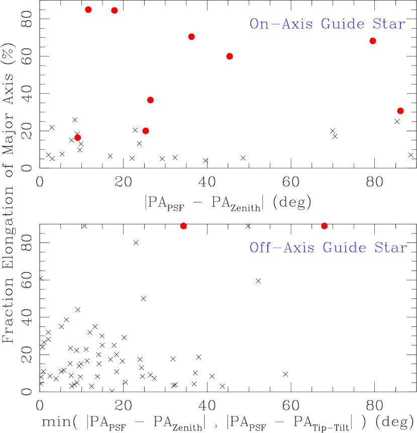
Figure 2.— Top: Fractional PSF elongation as a function of its alignment with the direction to zenith for independently-confirmed binary systems (red circles) and all other targets (black crosses) that served as their own tip-tilt guide star. Most non-binary sources appear to be roughly aligned with zenith, a trend which indicates that wind-induced telescope shake is common among our observations. All sources which are not known binary systems appear to have PSF elongations of $<$30%, which seems to be the ceiling for weather-induced effects. Bottom: A similar figure for targets which had off-axis tip-tilt guide stars, where we plot the elongation of the target PSF with respect to the closer of the angle to zenith or the angle to the tip-tilt. Tip-tilt anisoplanatism also seems to induce PSF elongation, but with the exception of firmly-detected binary systems and targets with very poor data quality, the ceiling for observational effects is $<$40%.

3.2. Photometry and Astrometry

We measured relative photometry and astrometry for candidate companions using the IRAF package DAOPHOT (Stetson, 1987). For source pairs with small separations, where the two PSF cores were not unambiguously resolved, we used the PSF-fitting ALLSTAR routine. For pairs with wider separations, we used the aperture photometry package PHOT. We analyzed each frame separately in order to estimate the uncertainty from the scatter between all frames; this also allowed us to reject some frames with subpar AO correction. Our final results represent the mean and standard deviation for all observations.

For the close binaries that we analyzed with ALLSTAR, we reconstructed the single-star PSF out of the merged binary PSF using the algorithm described in Kraus & Hillenbrand (2007c), which iteratively fits a template PSF to the primary and then subtracts the secondary to fit an improved estimate of the primary. For one triple system, UScoJ1607-2019, we chose instead to use the single secondary as a PSF template for fitting the close pair constituting the primary. This choice allowed us to clearly distinguish the close pair despite a separation ($\sim$50 mas) that was significantly lower than the PSF FWHM ($\sim$70 mas).

Our relative astrometric measurements were distortion-corrected using a new high-order distortion solution (Cameron 2008) that delivers a significant performance improvement as compared to the solution presented in the NIRC2 pre-ship manual. This distortion solution was derived from observations of a pinhole mask in the NIRC2 filter wheel, so it does not include any distortions introduced upstream of this point. The remaining residuals due to these uncorrected distortions are $\sim$5 mas for positions separated by $\sim$5–10″  (J. Lu, priv. comm.). We calibrated our photometry using the known 2MASS $K_{s}$ magnitudes for each of our science targets; these absolute magnitudes are uncertain by $\sim$0.1–0.2 magnitudes due to the intrinsic variability of young stars (resulting from accretion or rotation).

3.3. (Sub)stellar and Companion Properties

Stellar properties can be difficult to estimate, particularly for young stars, since pre-main-sequence stellar evolutionary models are not well-calibrated. The model-predicted masses of young stars could be systematically uncertain by as much as 20% (e.g., Hillenbrand & White, 2004), and estimates for individual stars could be uncertain by factors of 2 or more if their observed luminosities are biased by unresolved multiplicity or the intrinsic variability that young stars often display (from accretion or from rotational modulation of star spots). This suggests that any prescription for determining stellar properties should be treated with caution.

We estimated the properties of all of our sample members using the methods described in Kraus & Hillenbrand (2007a). This procedure combines the 2 or 5 Myr isochrones of Baraffe et al. (1998) and Chabrier et al. (2000) with the temperature scales of Schmidt-Kaler (1982) and (Luhman et al., 2003) to directly convert observed spectral types to masses. Relative properties (mass ratios $q$) for all binaries in our sample were calculated by combining these isochrones and temperature scales with the empirical NIR colors and K-band bolometric corrections of Kraus & Hillenbrand (2007b) to estimate $q$ from the observed flux ratio $\Delta K^{\prime}$.

For all binary systems, we have adopted the previously-measured(unresolved) spectral type for the brightest component and inferred its properties from that spectral type. This should be a robust assumption since equal-flux binary components will have similar spectral types and significantly fainter components would not have contributed significant flux to the original discovery spectrum. Projected spatial separations are calculated assuming the mean distance to the associations ($\sim$145 pc for both Upper Sco and Taurus; de Zeeuw et al., 1999; Torres et al., 2009). If the total radial depth of each association is equal to its angular extent ($\pm$8^o or $\pm$20 pc), then the unknown depth of each system within the association implies an uncertainty in the projected spatial separation of $\pm$14%. The systematic uncertainty due to the uncertainty in the mean distance of each association is negligible in comparison ($\lesssim$2%).

4. Results

4.1. Candidate Companions and Detection Limits

Our search for sources in the speckle-dominated regime (at separations $\gtrsim$1.5 times the PSF FWHM and extending to the edge of the detector; Section 3.1.1) yielded 45 candidate companions among the 78 young stars and brown dwarfs in our observed sample. All candidates within $\lesssim$1″of the target sit well above the 5$\sigma$ detection limit, so they all represent secure detections and do not seem to be spurious structures in the primary star’s PSF. We also found numerous possible detections with significance levels of 5–6$\sigma$ in this regime, but as we described in Section 3.2.1, all of these possible detections appear to be spurious. Our corresponding search for sources in the core-dominated regime (at separations of order the PSF FWHM; Section 3.1.2) yielded 9 targets with PSF cores consistently elongated by $>$40%. Many targets had PSF elongations below this limit, but as we discussed above, most appear to be distorted due to observational effects and not the presence of a companion. We address the membership probabilities of these candidates in Section 4.2.

In Table 3, we list our survey’s candidate companions and report their flux ratios, separations, and position angles. We also plot the flux ratio $\Delta$$K^{\prime}$ and the candidate companion brightness $K^{\prime}$ as a function of separation in Figures 3 and 4, respectively. Finally, in Figure 5, we show contour plots for the 12 candidate companions with separations $<$1″  and flux ratios of $\Delta$$K^{\prime}<4$; we do not show contour plots for wider systems because they are completely resolved, and we do not show any faint companions because few are likely to be bound companions. The vast majority of our wide-separation candidates are near the detection limits of our survey, in the brightness range where a real companion would fall below the deuterium-burning limit ($\sim$13 $M_{Jup}$), so we expect that almost all are unassociated field stars. However, a handful of planetary-mass companions have been identified around young stars and brown dwarfs (e.g., 2M1207b; Chauvin et al., 2004), so we must consider the possibility that some of the candidates in our survey are also extremely low-mass companions. We will present second-epoch observations that test the membership of these candidates in a future paper. In all cases, the high astrometric precision of Keck/NIRC2 ($\sigma\sim$1–2 mas) and the relatively large proper motions ($\mu\sim$20–30 mas/yr) allow for a test of common proper motion using observations from consecutive observing seasons.

Of the 54 combined sources from the speckle-dominated and core-dominated regimes, 11 had already been identified as candidate binary companions by past survey efforts, so we note these past identifications in Table 3. Three of our candidate companions merit special attention. V410 X-ray3 AB was identified as a candidate binary in our previous HST/ACS multiplicity survey based on a marginal elongation of its PSF, but the best-fit separation was well inside the HST diffraction limit for the $i^{\prime}$ and $z^{\prime}$ filters. By contrast, the system is almost resolved in our $K^{\prime}$ observations, and corresponding $JH$ images (Kraus 2009) clearly reveal V410 X-ray3 to be a genuine binary system. Two wide binary systems, USco 80 AB and UScoJ1607-2019 AB, were resolved to be hierarchical triples. USco 80 A is clearly resolved to be a close pair, while UScoJ1607-2019 A is marginally resolved.

The other 26 members of our sample have no resolved neighbors within our detection limits. These detection limits, which we derived using the methods described in Section 3.1 and list in Table 4, are extremely heterogeneous due to the wide range in observing conditions during our observing campaign. Some observations nearly achieve the expected limits for diffraction-limited images, while images from most of the other nights achieved significantly poorer conditions. We also note that our nominal detection limits for bound companions at wide separations was constrained by our followup efforts. We found many more faint candidates than we were able to follow up with second-epoch imaging, so we can not claim completeness beyond the maximum separation or flux ratio at which we have identified all of the field stars by testing for common proper motion.

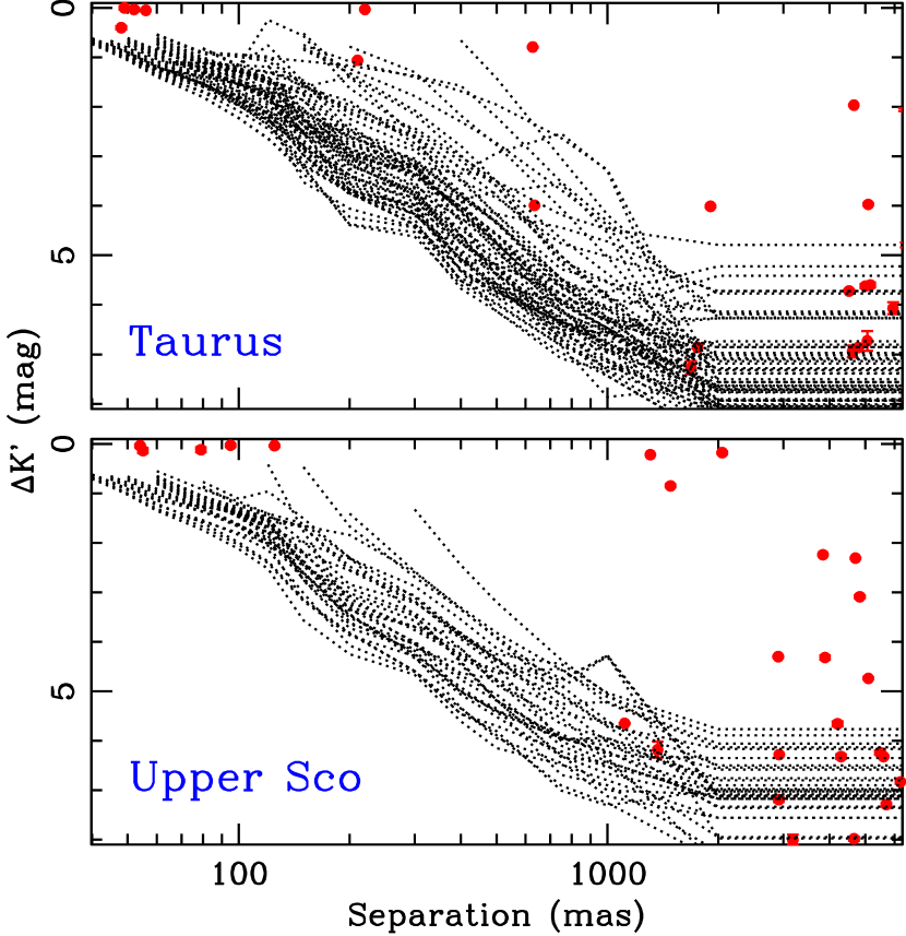
Figure 3.— Separation and flux ratio for each of the candidate companions in our sample. The top panel shows our results for the 53 Taurus members in our sample, while the bottom panel shows our results for the 28 Upper Sco members. Red circles denote the candidate companions that we have detected, while dotted lines show the inferred detection limits for all sources.

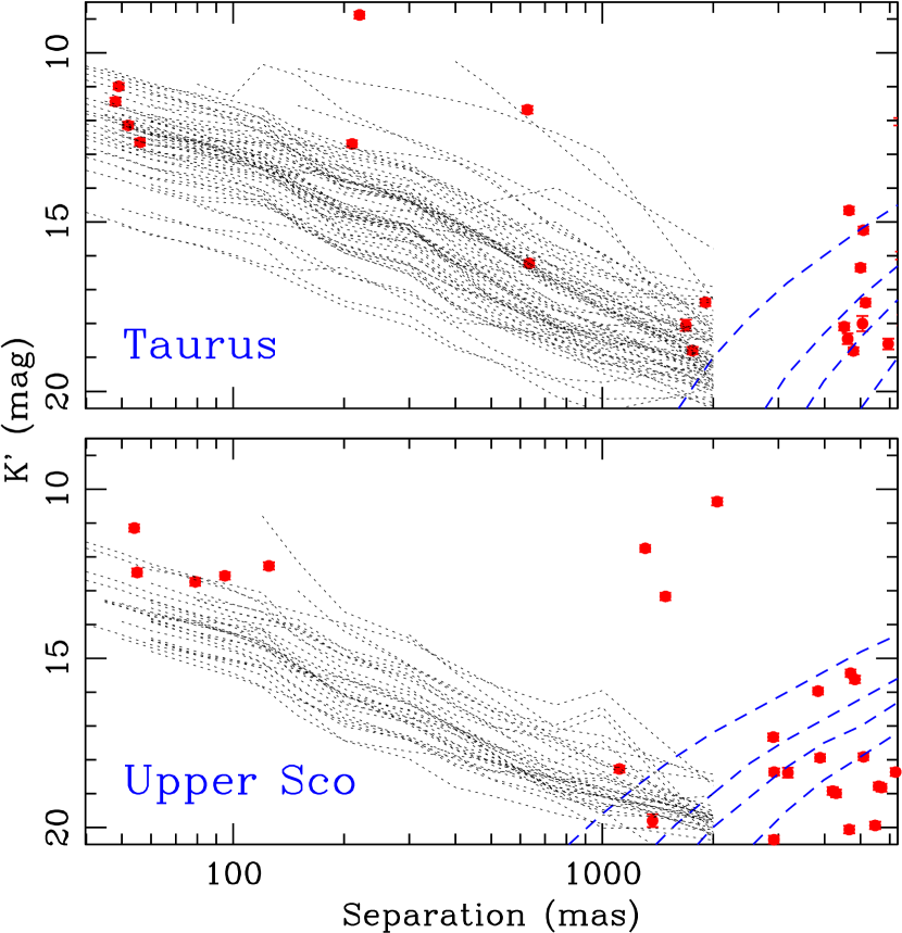
Figure 4.— Separation and apparent magnitude $m_{K^{\prime}}$ for each of the candidate companions in our sample. Red circles and dotted lines are defined as in Figure 3; blue dashed lines denote levels of constant contaminant density where we expect to find 1, 3, 5, or 10 background stars that are brighter and located at smaller projected separation.. We inferred these contamination rates using the star count models that we describe in Appendix A. All detection limits converge to the read-noise limit at separations of $>$2″, so we do not extend the limits beyond that separation since the lines would obscure the faint sources and the background contamination contours.

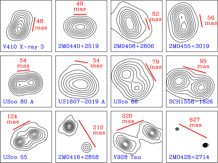
Figure 5.— Contour plots for the twelve binary systems we observed to have separations of $<$1″. The top row includes four close binaries ($<$100 mas) in Taurus, the middle row includes four close binaries in Upper Sco, and the bottom row includes four wider binaries ($>$100 mas) from both associations. In each case, we plot contours at 95% at the peak flux, and then in 10% increments until reaching the seeing-limited halo; images with poor AO correction therefore show fewer contours

4.2. Binary Systems and Field Stars

Companion searches must address the prospect of chance alignments with background stars, especially surveys with very deep detection limits. We are obtaining multi-epoch astrometry for several candidates in order to test for common proper motion, but we can use statistical arguments to determine which candidate companions require those followup observations. As we describe more fully in Appendix A, we have updated the Milky Way model of Bahcall & Soneira (1980) to predict star counts as a function of magnitude for the line of sight toward each of our targets; these models allow us to predict the field star contamination rate and thereby determine which companions have a significant probability of being background stars.

In Figure 4, we plot the joint magnitude-separation limits at which our models predict we should find 1, 3, 5, or 10 background stars among all the targets observed in that association. In both associations, our models predict that we should find $<$1 background star with $K\lesssim$15 within $<$5″, which suggests that all of the bright sources we observe well inside this limit are genuine companions. This limit agrees with our estimate based on 2MASS source counts in the direction of Taurus and Upper Sco (Kraus & Hillenbrand, 2007a), which found that all neighbors down to the 2MASS 10$\sigma$ limit ($K=14.3$) could be assumed to be bound association members out to separations of 3–5″.

The status of our fainter candidates is not as clear. Our models predict that we should find only one background star with separation $\rho$$<$2″  and brightness $K<$19 in Taurus, so the candidates inside this limit all seem very promising as potential analogs to 2M1207b. The background star density is higher in the direction of Upper Sco since it lies in the direction of the galactic center, so even with our smaller sample size, we still expect 3 chance alignments with $\rho$$<$2″and $K<$19. However, star count models are not well-constrained at $K\gtrsim$14 since the counts are dominated by low-mass halo stars, a population that is not as well-studied as the brighter disk stars. As a result, the contamination rate for faint stars could be uncertain by a factor of at least 2–3. It would be prudent to measure common proper motion for any candidate companion fainter than $K\sim$14, especially since any genuine companion would have $M<$10–20 $M_{Jup}$, making it an extremely compelling discovery. The predicted background star contamination rate rises quickly for separations $\gtrsim$3″, matching the many candidates we have discovered, so we provisionally adopt this separation as an outer limit at which it is worthwhile to test candidates for possible association. Future searches at wider separations should use seeing-limited data from publicly available surveys like UKIDSS, which will observe the majority of these targets in four NIR filters.

Finally, multiplicity surveys in young clusters and associations must also consider chance alignments between two unbound member stars. These chance alignments are extremely difficult to distinguish from genuine binary systems since all association members are young, at similar distance, and comoving to very high precision. The only solution is to treat their probability in a statistical sense, which we have already done in our treatment of wider binary systems (Kraus & Hillenbrand, 2009b). We found that the probability of a chance alignment between two young association members is negligible for separations $<$10″, so we will proceed under the assumption that any pair of young stars constitutes a genuine binary system.

In Table 5, we list the mass ratios and component masses that we infer for the candidate companions brighter than $K=14$ and closer than 3″  from their primary star, which we henceforth consider to be bound binary companions. For targets that were observed at multiple epochs, we list the independent estimates from each epoch. These properties were derived using the methods we describe in Section 3.3.

5. Characterizing Multiplicity at the Bottom of the IMF

The frequency and properties of multiple star systems offer important constraints of star formation processes, and the extreme disparity between the binary populations of the VLM population and higher-mass stars could provide a powerful test of star formation models. However, most of the large multiplicity surveys in the VLM regime have been conducted for old systems in the field. Constraints for young binary systems, especially those in dynamically primordial populations like Taurus and Upper Sco, are only now beginning to match the field surveys.

The archetypal concept of VLM multiplicity was established by a trio of high-resolution imaging surveys for nearby field targets. Bouy et al. (2003), Burgasser et al. (2003), and Close et al. (2003) all found that low-mass binaries are less common ($f\sim$10–15% for separations of $\rho$$\gtrsim$2–4 AU), more compact ($\rho$$\lesssim$10–20 AU), and more symmetric ($q\gtrsim$0.7–0.8, or $M_{sec}$$\sim$$M_{prim}$) than the corresponding population of solar-type binaries studied by Duquennoy & Mayor (1991). The scarcity and tightly-bound nature of low-mass binaries led to suggestions that this indicated past strong dynamical interactions, perhaps consistent with the embryo ejection hypothesis for brown dwarf formation (Reipurth & Clarke, 2001). However, the field population only allows an incomplete and muddled view of its primordial properties. The field represents a composite of many different formation environments, but it is probably dominated by stars formed in dense clusters (e.g., Lada & Lada, 2003), so it is difficult to disentangle any environmental effects, especially those tied to primordial stellar density. Field brown dwarfs are also subject to a mass-age degeneracy, which makes it difficult to infer mass-dependent trends, and the steep mass-luminosity relation makes it difficult to identify companions which are much less massive than their primary stars (Chabrier et al., 2000).

These complications can be avoided by studying multiplicity in nearby star-forming regions and young associations. These populations have homogeneous and better-constrained initial conditions, their known age allows for a (model-dependent) resolution of the mass-age degeneracy, and their youth corresponds to a very shallow mass-luminosity relation that improves sensitivity to low-mass companions. Furthermore, these results can be directly compared to simulated stellar populations (e.g., Bate 2012), as we discuss in more detail in Section 5.3. The only tradeoff is that these populations are more distant than nearby field stars, imposing a resolution penalty against the discovery of binaries with small separations. Preliminary surveys have indicated that the field paradigm, with infrequent and tightly-bound binaries, is broadly consistent with several different formation environments (Kraus et al., 2005, 2006; Konopacky et al., 2007; Ahmic et al., 2007). However, they also indicated a further dependence of separation and frequency on mass within the VLM and substellar regime, and these mass-dependent effects can only be explored with a large binary survey among targets with known ages.

5.1. Bayesian Inference and Binary Population Statistics

Binary population statistics are traditionally presented in terms of histograms of binary frequency versus separation or mass ratio, where the data is presented only for a range where the survey is complete. The analytic form of the preferred model is then fit to these histograms in order to infer the population properties. This approach has the virtue of simplicity, but estimating the probability density function (PDF) for the model’s scale parameters is often difficult, especially if there are covariances between parameters. This method also is manifestly inadequate for handling heterogeneous datasets. If different stars have different detection limits, such as from being observed with different methods or under different atmospheric conditions, then simple histograms can be constructed only by appealing to completeness corrections that are themselves poorly constrained.

A better solution for working with heterogeneous data is to adopt a Bayesian approach, where the scale parameters of the model are assigned a prior PDF and that PDF is modified by each observation. This method exploits Bayes’ theorem:

$$P(\theta|O)\propto P(O|\theta)P(\theta)$$ (1)

where $\theta$ represents the “model” (a set of scale parameters describing the functional form), $O$ represents the observation, $P(\theta|O)$ is the posterior PDF for the model (as a function of its parameters) given the data, $P(O|\theta)$ is the probability of obtaining an observation as a function of the model parameters, and $P(\theta)$ is the prior PDF for the model (again, as a function of its parameters). In cases with multiple observations (such as a survey of many targets), the posterior function for one observation is then used as the prior function for the next observation.

Allen (2007) (hereafter A07) developed the relevant techniques for applying Bayesian statistics to VLM multiplicity, and we have largely adopted his approach in this work and a parallel survey of solar-type stars in Taurus (Kraus et al., 2011). We specifically describe the binary population in terms of a binary fraction $F$, a power-law mass ratio distribution with exponent $\gamma$, and a log-normal separation distribution with mean $\log(s)$ and standard deviation $\sigma$_log(s). We have adopted the same Poisson likelihood function as A07, but we will use a moderately different set of prior distributions. As for A07, we use constant priors for $\gamma$ and $\log(s)$. However, A07 seem to state that scale invariance requires the optimal unbiased prior for $\sigma_{\log(s)}$ to be proportional to $1/\sigma_{\log(s)}$, whereas it actually should be proportional to $1/\sigma_{s}$, or constant in $\sigma_{\log(s)}$.

The difference for $F$ is more subtle. A07 used a prior proportional to $1/F$, which was suggested to be suitable for a Poissonian variable. As we discussed in Kraus et al. (2011), the Poisson case is sometimes appropriate if there are many high-order multiples, though our newest analysis actually uses the Jeffries prior that is proportional to $1/\sqrt{F}$ (Kraus et al., in prep). However, binary companions exclude other binary companions in similar orbits (spanning at least a decade of semi major axis), so they are are not genuinely Poissonian. As we show below, ultra cool binaries typically only have small projected separations, perhaps not spanning much more than a decade of semi major axis, so the exclusionary effect should be quite significant. We are attempting to use completely uninformed priors for this analysis, but a more sophisticated prior that declines more quickly than $1/\sqrt{F}$ should considered for future analyses.

Another significant difference between our analysis and that of A07 is that we directly model the projected separation distribution, whereas A07 used the semimajor axis as a model parameter and then extrapolated a projected separation distribution using an assumed eccentricity distribution and randomly-distributed inclinations and phase angles. The eccentricity distribution for binary systems is still largely unconstrained for the separations and mass ranges that we consider, but most likely eccentricity distributions yield a separation distribution that is directly proportional to the semimajor axis distribution. As such, our results can be directly related to theoretical semimajor axis distributions once the eccentricity distribution is predicted by theory or measured by future surveys. We have also omitted the volume-completeness correction used by A07 to compensate for the overluminosity of similar-brightness binaries. The discovery surveys for most of our sample members were spatially limited, not flux- or volume-limited, so binary systems were equally likely to be detected. The high-resolution imaging techniques used in past surveys were themselves flux-limited, but we chose our LGSAO sample in part to compensate for this limit, so it should not significantly influence our results to invoke detections and detection limits from those past surveys where needed.

Our specific implementation of Bayesian analysis follows that of A07, defining two-dimensional functions of projected separation $\log(s)$ and mass ratio $q$ that denote the number of observations sensitive to each set of $\log(s)$ and $q$ (the “window function”) and the corresponding number of companions with that set of parameters. We iterated our calculation over all mass ratios from 0 to 1 in steps of 0.01 and over all values of $\log(s)$ between 0.5 and 3.6 dex in steps of 0.1 dex; this range of $\log(s)$ was chosen to encompass the full range of projected (physics) separations for which imaging observations are sensitive, from 3 AU (due to the minimum resolution limit of the most sensitive surveys; Kraus et al. 2005, 2006) to 4500 AU (the maximum projected separation for which we have eliminated background star interlopers for most targets; Kraus & Hillenbrand 2007, 2009).

Our own sample comprises the vast majority of available measurements in the VLM regime ($M\lesssim$0.15 $M_{\sun}$), but almost all of the measurements for higher-mass stars must be adopted from previous surveys. As we describe in Appendix B and list in Table 7, we have specifically adopted the detections and detection limits for all stars with $M\lesssim$0.5 $M_{\sun}$ for previous surveys of Taurus-Auriga (Ghez et al., 1993; Simon et al., 1995; Kraus et al., 2006; Konopacky et al., 2007), Upper Sco (Köhler et al., 2000; Kraus et al., 2005; Biller et al., 2011), and Cha-I (Ahmic et al., 2007; Lafrenière et al., 2008). In each case, we converted the measured angular separations (in mas) and flux ratios (in $\Delta$$m$) for their detections and detection limits into physical quantities (separations in AU and mass ratios) using the same methods that we applied to our own sample. This ensures a uniform set of inputs for our analysis, whereas each survey’s inferred system properties were derived using different combinations of association distances/ages and pre-main sequence stellar evolutionary models.

Past studies have indicated that multiple star formation might be a mass-dependent process, so we have divided our sample into several bins. The stellar/substellar boundary represents a natural breaking point since it corresponds roughly to the M/L boundary for field objects, allowing for natural comparison to field samples. As we have indicated in our studies of solar-type multiplicity and wide multiplicity, systems with primary masses of $\gtrsim$0.5 $M_{\sun}$ tend to have fundamentally different binary parameters, featuring a log-flat separation distribution and many very wide systems, so we have adopted this limit as the maximum for consideration in our sample. The desire for similar number statistics per bin therefore dictated four mass bins of similar width: $<$0.07 $M_{\sun}$, 0.07–0.15 $M_{\sun}$, 0.15–0.30 $M_{\sun}$, and 0.30–0.50 $M_{\sun}$. A more rigorous treatment might incorporate a mass dependence directly into our fit parameters ($F$, $\gamma$, $\log(s)$, and $\sigma$_log(s)), but in the absence of any theoretical guidance on the functional form of this mass dependence, we will defer such analysis to a future study.

Our Bayesian analysis yields a PDF for all possible “models” that is defined across four dimensions, so we can not present the full results in a two-dimensional medium. However, any two parameters for which the covariance is small can be presented separately without discarding information. This independence allows us to instead present the results as a series of lower-dimensional surfaces, where PDF is integrated across the uncorrelated parameters in order to flatten its dimensionality. As we describe in the next section, our results can be described with a manageable number of 2D or 1D surfaces.

Finally, it is impossible to define a true PDF with only null detections, so we can not use this analysis for the lowest-mass bin ($M<0.07$ $M_{\sun}$) since it includes no resolved binary systems. Our choice to use generic conjugate priors does not disallow arbitrarily extreme values, such as small mean separations or steep power laws. If we do not have enough constraints (i.e. detected binaries) to force the PDF to zero at all extrema of the scale parameters, then the integrated probability will diverge and render the PDF unnormalizeable. Since we can not estimate a well-defined probability for any particular set of parameters being “correct”, we instead must settle for a weaker result: the probability that a given set of parameters would have yielded our null detection. This measurement is equally valid for ruling out parameter space, but does not carry any explicitly affirmative value; regions where the model is less improbable are not necessarily regions where the model is probable. The act of “flattening” the PDF to visualizable 1D or 2D figures is also not defined for this type of constraint, so in figures where the PDF for higher-mass bins is flattened, we will instead show a cross-section through the lowest-mass PDF where we adopt the field T dwarf parameters suggested by Burgasser et al. (2006): $\log(s)$$\sim$0.6, $\sigma$_log(s)$\sim$0.3, and $\gamma$$\sim$4.2.

5.2. The Mass-Dependent Parameters of the Multiple Star Population

The four-dimensional posterior PDF for our Bayesian analysis can be flattened to present six two-dimensional probability surfaces and four one-dimensional probability curves, but to convey the useful conclusions, we only need surfaces for covarying parameters and curves for non-covarying parameters. For our results, we will present two probability surfaces ($F$ versus $\log(s)$ and $F$ versus $\sigma$_log(s)) and one probability curve ($\gamma$).

In general, we found little covariance between $\gamma$ and any other parameter, which is largely a result of the shallow mass-luminosity relation for young stars and brown dwarfs; at a given separation, most observations are either unable to detect any companions or sensitive to companions with almost all mass ratios. There is significant covariance between the binary frequency $F$ and the two parameters in the separation distribution, $\log(s)$ and $\sigma$_log(s). This degeneracy results from the inner working angle for most of the input datasets ($\sim$5–10 AU) being of similar order as the mean separation, since our measurements are consistent with a range of binary frequencies as long as an appropriate fraction of the companions are “hidden” inside the detection limit with a smaller mean separation and correspondingly wider standard deviation. As we discuss further in Section 5.3, a comparison to similar constraints from simulated stellar populations (e.g., Bate 2012) also can provide a direct test of star formation models and indicate future directions for their improvement.

5.2.1 Frequencies and Separation Distributions for Stellar Multiplicity

In Figure 6, we show the PDFs for our three stellar-mass bins as projected onto the $F$-$\log(s)$ and $F$-$\sigma$_log(s) planes. In the two lower-mass bins (0.30–0.15 $M_{\sun}$ and 0.15–0.07 $M_{\sun}$), there is a significant degeneracy between the overall binary frequency and the mean separation, where a smaller mean separation is paired with a higher frequency. This degeneracy is unavoidable when fitting a normal distribution whose mean is near or outside the fitting region; the first derivative (i.e. the slope) of the distribution across the fitting region yields the standard deviation with little ambiguity, but distinguishing between the total amplitude of the curve and the distance (in standard deviations) to the mean requires measurements of both the number of measurements and the second derivative (i.e. the change in slope) across the fitting region. Measuring each successive derivative requires either more $S/N$ or a wider fit regime. The highest-mass bin also shows some degeneracy with separation, but not to the same extent since its mean separation is outside of the typical inner working angles for many of the input surveys.

The $F$-$\log(s)$ locus in the highest-mass bin (0.3–0.5 $M_{\sun}$) is clearly distinct from the loci of the two lower bins (0.30–0.15 $M_{\sun}$ and 0.15–0.07 $M_{\sun}$), as its 90% confidence region does not overlap with the same regions for the other bins. This indicates that the mean separation and/or the binary frequency are significantly higher for 0.3–0.5 $M_{\sun}$ stars. The strong degeneracies seen for the lower-mass bins make it difficult to draw any strong conclusions, but it appears that the frequency and/or mean separation for binary systems declines from the 0.15–0.30 $M_{sun}$ regime to the 0.07–0.15 $M_{\sun}$ regime. As we discuss in Section 5.2.2, this decline seems to continue in the substellar bin, though our constraint on its relative magnitude in each parameter is even weaker since we only have a null detection for that mass bin. The $F$-$\sigma$_log(s) loci are not as easy to interpret; the middle locus is biased to a larger standard deviation, but this might be the result of having 4 probable binary systems with separations of $>$1000 AU; if some of these pairs of stars are actually chance alignments of unrelated association members, then removing them would reduce the standard deviation and the mean separation by a significant amount.

The frequency-separation degeneracy must be addressed before we can draw any stronger conclusions. The most direct solution would be to increase the number statistics in our existing program, yielding a better estimate of the high-order derivatives in the separation distribution. However, this endeavor would be very observationally expensive; simulations show that even doubling our sample would not decrease the length of the degenerate locus, only its width. A less direct solution would be to expand the range of separations over which the distribution is constrained, either by observing at higher resolution (sampling more of the core separation distribution) or by searching for spectroscopic binaries (constraining the other wing of the separation distribution). We suggest that an RV survey would be significantly cheaper since it can exploit the multiplexing of wide-field multi-object spectrographs, plus the separation-frequency degeneracy that results from an RV survey’s outer working angle should be perpendicular to the degeneracy from imaging surveys’ inner working angle. Such surveys are currently being pursued for nearby young populations like the sigma Ori cluster (Maxted et al., 2008) and the ONC (Tobin et al., 2009), and their results could be modeled with similar Bayesian techniques in order to produce constraints analogous to those shown in Figure 6. However, such a modeling effort is beyond the scope of the current work.

Finally, although Bayesian inference allows us to estimate the most general limits on the binary population, the degeneracies in those limits make it difficult to straightforwardly grasp the differences in our subsamples. We address this by forward-modeling from our four-dimensional PDF back into the range of separations and mass ratios where our observations could detection companions around most of our targets. The net result of this extrapolation is to implement a minor correction for incompleteness, but rather than adopting one assumed form for the underlying distributions, we implicitly integrated the correction over all possible distributions, weighted by the probability for each distribution. To this end, we have integrated over the entire four-dimensional PDF of each mass subsample to extrapolate the binary frequency at separations of 8–5000 AU and spanning all mass ratios of $0<q<1$. We find that in order of declining mass, our three subsamples (0.5–0.3 $M_{\sun}$, 0.30–0.15 $M_{\sun}$, and 0.15–0.07 $M_{\sun}$) have binary frequencies of $50^{+10}_{-9}\%$, $29^{+7}_{-6}\%$, and $21^{+7}_{-6}\%$ in this range of parameter space.

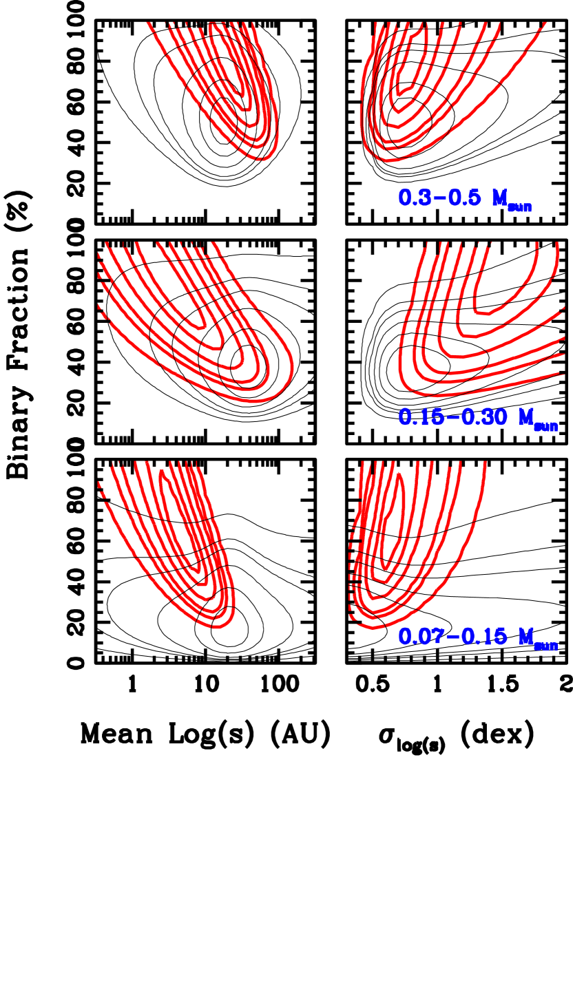
Figure 6.— Posterior probability density functions for three mass ranges of stellar binaries. In each row, we plot the probability surface as projected onto the $F$-$\log(s)$ and $F$-$\sigma$_log(s) plane, showing contours that enclose total probability densities of 25%, 50%, 75%, 90%, 95%, and 99%. Red thick lines denote contours for our sample of observed binaries, while thin black lines denote contours for the synthetic binary population generated by Bate (2012) in a radiative SPH simulation (Section 5.3).

5.2.2 Limits on Substellar Multiplicity

As discussed above, we can not directly constrain the parameters of the substellar binary population because we did not discover any such binaries in our sample. However, we can estimate the probability of a null detection as a function of the four parameters in our model, ruling out a large portion of parameter space. In Figure 7, we show our null detection probability surfaces for the substellar mass bin in the $F$-$\log(s)$ and $F$-$\sigma$_log(s) planes. We can’t integrate over the unplotted dimensions of our PDF since the integral diverges, so we instead show cross-sections for the most likely values as inferred by Burgasser et al. (2006): $\log(s)$$\sim$0.6, $\sigma$_log(s)$\sim$0.3 dex, and $\gamma$$\sim$4.2. We chose these parameters because the T dwarf sample studied by Burgasser et al. more closely matches our mass range than the full sample of MLT dwarfs studied by A07.

We find that for the given values of $\sigma$_log(s) and $\gamma$, we can not rule out any mean separations $\lesssim$1 AU at $>$50% confidence. However, we can rule out combinations of increasing mean separation and decreasing binary frequency; if the mean separation is 2 AU, then the binary frequency is $<$11% at 50% confidence and $<$38% at 90% confidence. If the mean separation is 4 AU, which is the maximum value consistent with the results of Burgasser et al., then the corresponding frequency limits are $<$4% and $<$11%, respectively. Conversely, if the total binary frequency is $\sim$20%, then the 50% and 90% confidence limits on the mean separation are 1.6 AU and 2.8 AU. The corresponding probability surface for $\log(s)$$\sim$0.6 and $\gamma$$\sim$4.2 is strongly concentrated at low frequencies since this mean separation is very close to the inner working angle of our LGSAO survey, and therefore at least half of all companions should have been detectable.

In summary, all of these limits for the substellar regime are extremely discrepant with respect to the confidence intervals for the higher-mass subsamples, which indicates that the the mass-dependent tightening of binary systems continues into the substellar regime. There are no well-defined and observationally-supported models for how low-mass binary systems form, so it is difficult to infer the underlying justification for the continued decline of system separations and/or frequencies into the substellar regime. However, the trend for declining separations and frequencies in the field appears to be established at very early ages and must result directly from the formation process.

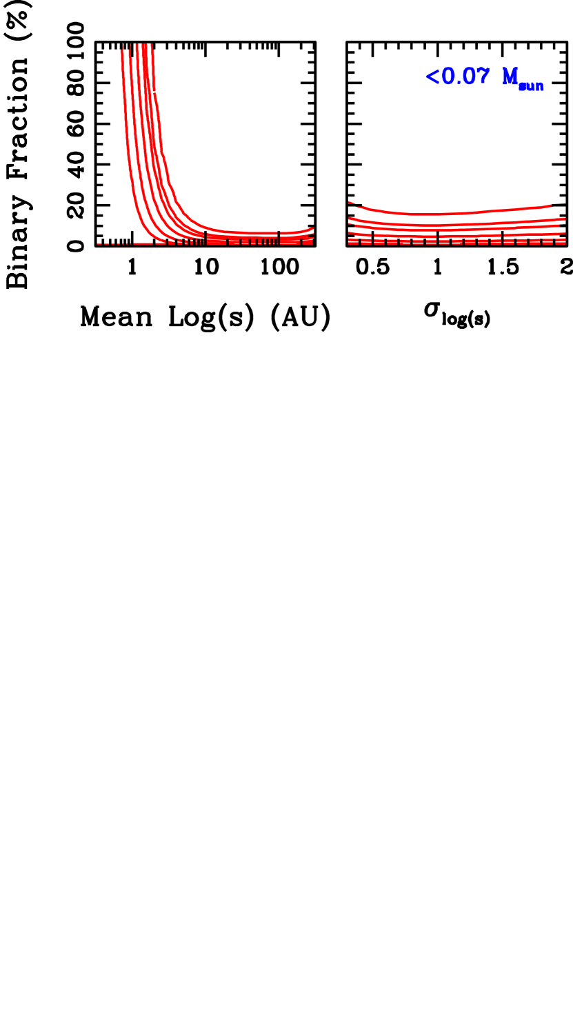
Figure 7.— As in Figure 6, but for our substellar subsample. The posterior PDF can not be normalized, so we can not plot contours of enclosed total probability density or integrate across the unplotted parameters. We instead plot confidence contours on the probability surface for a null detection, and show cross-sections through the four-dimensional PDF at the most likely values inferred by the T dwarf multiplicity study of Burgasser et al. (2006): $\log(s)$$\sim$0.6, $\sigma$_log(s)$\sim$0.3 dex, and $\gamma$$\sim$4.2. We chose these parameters because the T dwarf sample studied by Burgasser et al. more closely matches our mass range than the full sample of MLT dwarfs studied by A07.

5.2.3 Mass Ratio Distributions

In Figure 8, we show the PDFs for our three stellar-mass bins as projected onto the $\gamma$ axis; we do not show any results for the substellar-mass bin because our null detection does not yield a useful constraint on its mass ratio distribution. Unlike for Figures 6 and 7, we decided to project the PDF onto an axis instead of a plane in order to display our constraints on the mass ratio distribution. There is no significant covariance between our constraints on $\gamma$ and those for other parameters, so this choice simplifies our presentation.

The 0.3–0.5 $M_{\sun}$ subsample has a best-fit slope of $\gamma$$=+0.18$${}^{+0.33}_{-0.30}$, a value which is consistent with the linearly-flat mass ratio distribution found for higher-mass stars in young associations (Kraus et al., 2008, 2011). By contrast, the 0.15–0.30 $M_{\sun}$ subsample has a steeper slope of $\gamma$$=+1.02$${}^{+0.59}_{-0.52}$, a value intermediate between the flat slope of higher-mass stars and the typically very steep power laws ($\gamma$$\sim$2–4) seen for late-M stars and L/T brown dwarfs in the field.

Finally, the 0.07–0.15 $M_{\sun}$ subsample has a best-fit slope that is similar to the 0.15–0.30 $M_{\sun}$ bin, albeit with a very wide confidence interval, yielding $\gamma$$=0.96$${}^{+0.70}_{-0.59}$. This result at first appears to contradict the overall trend for a steeping mass ratio distribution with declining mass that is seen in the field and would seem to lead from the 0.15–0.30 $M_{\sun}$ subsample. However, closer inspection of the sample suggests a possible solution. Of the 7 binary systems in the 0.07–0.15 $M_{\sun}$ bin with projected separations of $\lesssim$20 AU, all have mass ratios of $\gtrsim$0.5. By contrast, of the 5 binary systems with projected separations of $\gtrsim$25 AU (GG Tau B, CFHT-Tau-17, and CFHT-Tau-18 in Taurus, Hn 13 in Cha-I, and RX J1558.1-2405b in Upper Sco),all but Hn 13 have a mass ratio of $\lesssim$0.5. The corresponding limits on the mass ratio power-law exponent are $\gamma=4.0^{+1.9}_{-1.6}$ for the closer subset and $\gamma=-0.3^{+0.7}_{-0.5}$ for the wider subset.

This trend is particularly intriguing because the five wider systems seem to approach or exceed the mass-maximum separation limit observed for field systems by Burgasser et al. (2003), who observed that for VLM binary systems in the field, there is a mass-dependent upper envelope to binary system separations, $a_{max}\sim$1400$M_{tot}^{2}$. The five systems have typical total masses of $\sim$0.15 $M_{\sun}$, corresponding to maximum “allowed” separations of $\sim$30 AU. As such, they appear to unusual in both their separation and their mass ratio.

It is tempting to consider whether the markedly different mass function for wider VLM binary systems is a result of a different formation history. For example, wider binary systems most likely form earlier in the collapse of the progenitor molecular core. At these earlier stages, there is still more material left in the circumstellar envelope that might preferentially accrete onto the more massive binary component, driving the mass ratio further from unity. By contrast, close binary systems most likely form in the final stage of collapse, after much of the circumstellar envelope has been accreted into the central mass and little would remain for preferential accretion. Thus, if fragmentation tends to yield similar-mass components, then the epoch of fragmentation would dictate how far the mass ratio could evolve from unity. Since lower-mass binary systems also tend to have smaller separations, this would naturally lead to the trend for lower-mass binaries to have mass ratio distributions which are increasingly peaked at unity.

This model does not explain why these systems do not have analogs in the field, so we must appeal to a separate trend to justify their absence. Most of our sample is drawn from environments that are much less dense than typical star clusters; indeed, all of our targets are in loose associations that are unbound and should disperse within the next 10–50 Myr. By contrast, most stars form in denser clusters (Lada & Lada, 2003) that are much more dynamically active and will ionize loosely-bound binary systems. For example, the separation distribution for solar-mass binary systems is truncated at separations of $\sim$300 AU in young clusters like the ONC (Köhler et al., 2006) and at $\sim$100 AU in older clusters like Praesepe (Patience et al., 2002). VLM binary systems in Praesepe with equivalent binding energy would have separations a factor of $\sim$3 lower ($\sim$30 AU). Therefore, these systems might have counterparts in denser clusters, but those counterparts could be disrupted into their component singleton stars before reaching the field.

Finally, we must consider a more prosaic explanation as well. All of our targets are located at distances of $\sim$140 pc, so we can not resolve binary systems closer than $\sim$5–10 AU. It is possible that our “unusually wide” binary systems are actually hierarchical multiples, where one component of the wide pair appears fainter (and thus less massive) because it is actually a close double comprised of two stars that each contain approximately half the mass of the primary. This would yield a total mass ratio close to unity in the wide pair, plus the higher total mass would allow for a correspondingly wider separation without violating the $a_{max}$-$M_{tot}$ relation. Large field surveys are starting to uncover a significant number of the very rare systems that appear at first to violate this relation (Caballero, 2007; Artigau et al., 2007; Radigan et al., 2009; Dhital et al., 2010)], but followup high-resolution imaging has shown that at least some of them are hierarchical triples or even quadruples (Law et al., 2010).

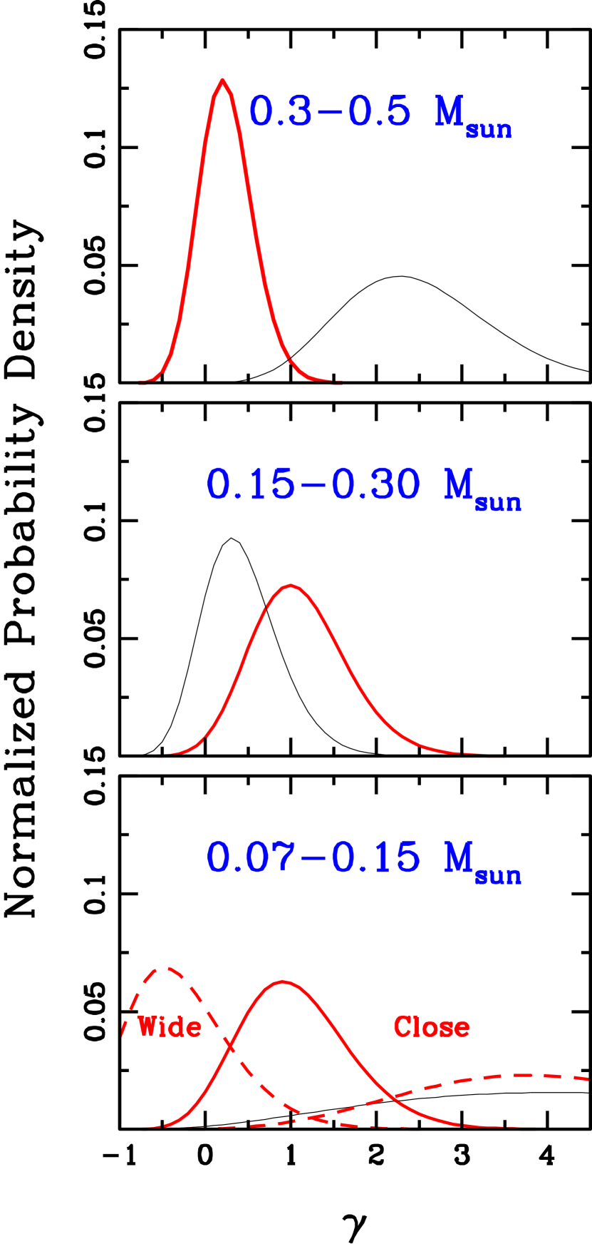
Figure 8.— Posterior probability density functions for three mass ranges of stellar binaries in our sample. In each row, we plot the probability curve as projected onto the $\gamma$ axis, denoting our confidence interval on the power-law exponent for the mass ratio distribution. As we discuss in the text, we also show separate fits in the 0.07–0.15 $M_{\sun}$ subsample for systems with separations of $>$25 AU (5 systems) and $<$25 AU (7 systems); close binary systems have a mass ratio distribution that is strongly peaked at unity, while four of the five wider binary systems have mass ratios of $<$0.5. As for Figure 6, our observational results are shown with thick red lines, while the synthetic population of Bate (2012) is shown with thin black lines (Section 5.3). The two separation regimes in the 0.07–0.15 $M_{\sun}$ subsample are denoted with red dashed lines.

5.3. Comparison to Star Formation Models

Smoothed particle hydrodynamic simulations are now capable of producing synthetic populations of young stars with statistically robust sizes (e.g., Bate 2009; Offner et al. 2010; Bate 2012), including samples of synthetic binaries that are equivalent in size to our observed samples of real systems. These synthetic binary populations provide a natural comparison sample for the results of our survey. The only synthetic population large enough to investigate mass-dependent trends was recently reported by Bate (2012), who simulated a cluster of $183$ stars and brown dwarfs, including $42$ multiple systems. Their simulation only ran for $2\times 10^{5}$ yr (due to computational expense), and had to end before the cluster dispersed all of its gas or became unbound, so the synthetic population likely was still evolving at the conclusion. However, it still provides an illustrative comparison sample. To produce a direct comparison, we have subjected their binary sample to the same Bayesian formalism as our observed sample, with the caveats that we set no detection limits (since all binaries are known) and we treated the semimajor axis as equivalent to the projected separation (since they are statistically equal to within nearly unity; Dupuy et al. 2011).

In Figures 6 and 8, we plot the confidence intervals corresponding to the posterior PDF as marginalized to the ($F$,$\mu_{\log(\rho)}$) and ($F$,$\sigma_{\log(\rho)}$) planes and the $\gamma$ line. These comparisons show that simulations reproduce a binary population that is broadly similar to that seen in observations; binaries have approximately the correct frequency, semimajor axes, and companion masses. This consistency is especially intriguing because the simulated environment is much denser than the regions we have observed, and hence dynamical interactions shape the synthetic population to a much greater degree. A more detailed comparison shows that not all features are consistent, though.

The simulations reproduce the most distinctive feature of real binary populations: a binary frequency which declines with decreasing primary mass. However, the separation distribution does not show the corresponding trend toward smaller semimajor axes, with a mean separation of $\sim$20–40 AU across the entire mass range. Furthermore, the standard deviation of the separation distribution only declines in the least massive bin, where it denotes a paucity of binaries at both $>$100 AU (in agreement with observations) and $<$5 AU (in sharp contrast with observations). The mass ratio distribution also does not match the expected trend for lower-mass systems to have mass ratios near unity. The lowest-mass bin shows a very strong bias toward such systems, but the highest-mass bin also shows a similar bias.

These discrepancies might be a result of not following the binary formation process to its conclusion. Accretion of additional circumstellar material should further modify the masses of the binary companions, and their semimajor axes also could be modified if the specific angular momentum of the accreted material is much higher or lower than for the binary components. Furthermore, dynamical interactions should disrupt or harden binary systems, and both effects would preferentially bias lower-mass binaries to have smaller semimajor axes than higher-mass binaries. The use of sink particles (with radius $r=0.5$ AU) also could affect processes occurring on AU scales, inhibiting the simulated production of tight binary systems.

If longer simulations can not improve the level of agreement, then it might suggest that other changes are required. The simulations now incorporate radiative feedback (Bate 2009; Bate 2012), and other simulations have suggested that magnetic fields are not likely to be significant on small scales (Price & Bate 2009). One possible avenue is to simulate different initial conditions. The simulations of Bate (2012) currently begin with an isothemal sphere of uniform density, which does not match the configurations seen for pre-stellar environments like the Pipe Nebula (e.g., Lada et al. 2009). Another possible variable to change is the turbulent power spectrum, which might affect the properties of binary systems (e.g., Goodwin et al. 2004).

6. Conclusions

We have presented the results of a large-scale survey of multiplicity at the bottom of the IMF in several nearby young associations. We have confirmed the overall trend observed in the field for lower-mass binary systems to be less frequent and more compact, including a null detection for any substellar binary systems with separations wider than $\sim$5–10 AU. In the stellar-mass regime, we confirm that the binary frequency and binary separations decline between masses of 0.5 $M_{\sun}$ and 0.08 $M_{\sun}$, though a degeneracy between the binary frequency and the mean binary separation make it difficult to distinguish the degree of the decline in each parameter. We also confirm that the mass ratio distribution becomes progressively more concentrated at $q\sim$1 for declining masses. However, we also note that a small number of systems appear to have unusually wide separations and low mass ratios for their system mass; this could indicate a secondary channel for low-mass binary formation, though unresolved high-order multiplicity could explain the unusual nature of some systems. Finally, we compare our results to synthetic binary populations generated by SPH simulations, finding that while models now reproduce the mass-dependent frequency of multiple systems, differences remain in the mass-dependent separation and mass ratio distributions.

7. Appendix A: A Model for Star Counts in the K Band

The use of star count models was pioneered by Bahcall & Soneira (1980) in order to study the structure of the Milky Way. Their procedure invoked a simple two-component model of the galaxy (composed of a disk and a spheroid) to characterize the density of stars as a function of position in the galaxy. The integrated luminosity function along any sightline through this distribution would then yield the number of stars as a function of magnitude for that location on the celestial sphere. The model has since been updated to include two disk components, the thin and thick disks (e.g., Gilmore & Reid, 1983), as well as separate components for the bulge and halo (e.g., Jackson et al., 2002).

Bahcall & Soneira originally used observational star counts in order to determine the scale heights and scale radii for each component of the galaxy. However, this process can also be inverted; given an adopted luminosity function and a set of scale heights and scale radii, it is possible to predict the number of stars per magnitude for any arbitrary position on the sky. We have developed an updated version of the Bahcall & Soneira models in order to predict faint source counts in our K band observations, characterizing the rate of background star contamination.

We adopted our K-band luminosity functions from several sources in the literature. We directly invoked the well-known K-band luminosity function for field giants as described by Mamon & Soneira (1982). The luminosity function for field dwarfs has only been measured in other filters, so we invoked the V-band luminosity function for A–K dwarfs from Reid et al. (2002), the J-band luminosity function for M0–M6 dwarfs from Reid et al. (2003), and the J-band luminosity function for M7–L8 dwarfs from Cruz et al. (2007). In each case, we used the magnitude-SpT relations of Kraus & Hillenbrand (2007b) and the color-SpT relations of Bessell & Brett (1988) to calculate the corresponding K-band luminosity function.

The scale parameters for Milky Way structural distributions, and even the functional forms themselves, have been updated numerous times since Bahcall & Soneira derived their original estimates. We have chosen to characterize the two disk components using exponential scale heights and scale radii and the halo using a power-law scale exponent and an oblate axis ratio. We did not fit the bulge because its triaxial distribution is still somewhat uncertain and because all of our targets are $>$20^o from the Galactic Center. Thus, the resulting functional form is:

$$\rho(R,Z)=\rho(R_{\sun},0)\times\lgroup\exp\left(\frac{R_{\sun}-R}{L_{thin}}-\frac{Z}{H_{thin}}\right)+$$

$$f_{thick}\exp\left(\frac{R_{\sun}-R}{L_{thick}}-\frac{Z}{H_{thick}}\right)+$$

$$f_{halo}\left(\frac{R_{\sun}}{\sqrt{R^{2}+(Z/q_{halo})^{2}}}\right)^{n_{halo}}\rgroup$$

where $R$ and $Z$ are cylindrical Galactocentric coordinates, $R_{\sun}$ is the solar Galactocentric radius, $f_{x}$ denotes the normalized density of each component in the solar neighborhood (relative to the thin disk), $L_{x}$ denotes a scale radius, $H_{x}$ denotes a scale height, $q_{halo}$ is the oblate axis ratio for the halo, $n_{halo}$ is the power law exponent for the halo, and $\rho(R_{\sun},0)$ is the present-day mass function in the solar neighborhood.

The parameters for the disks and halo were estimated most recently by Jurić et al. (2008), using positions and photometric distances for stars from the Sloan Digital Sky Survey to directly fit the three-dimensional distributions of stars. Based on the distribution of disk M dwarfs, they found that the two disk components have scale heights of $H_{thin}=300$ pc and $H_{thick}=900$ pc and corresponding scale radii of $L_{thin}=2600$ pc and $L_{thick}=3600$ pc; the normalized density of thick disk stars in the solar neighborhood is $f_{thick}=0.12$. Based on the distribution of main-sequence turnoff stars, they found that the halo has an axis ratio of $q_{halo}=0.64$, a radial power-law exponent of $n_{halo}=-2.8$, and a normalized local density of $f_{halo}=5\times 10^{-3}$.

However, we found from comparisons to 2MASS that the parameters of Jurić et al. (2008) yielded a radial gradient in thin disk density that was too steep, overestimating the density of thin disk stars toward the Galactic center and underestimating the density toward the Galactic anticenter. Based on observations at very high galactic latitudes, we found that their parameters also overestimated the number of thick disk stars. Older studies (e.g., Chen et al., 2001; Siegel et al., 2002) have found that a larger thin disk scale radius (similar to the thick disk, $\sim$3600 pc) and a lower fraction of thick disk stars in the solar neighborhood ($\sim$0.06) produce acceptable fits for other datasets. These values also fit our data, so we have adopted them instead.

Finally, we accounted for dust obscuration by assuming that the dust density approximately traces the thin disk; this result is roughly consistent with observations of nearby edge-on disk galaxies (e.g., Bianchi, 2007). The total integrated extinction along a sightline (in magnitudes) is then proportional to the total integrated dust density. We normalized the extinction by assuming that dust causes one magnitude of V band extinction per kiloparsec in the Solar neighborhood, (0.11 magnitude of K band extinction, based on the reddening law of Schlegel et al. (1998)). All of our science targets are at intermediate galactic latitudes (15^o$<|b|<$30^o), so the total effect is $\lesssim$0.5 mag in all cases.

We did not include the effect of residual molecular cloud material around our science targets because extinction measurements from the literature only include foreground obscuration, not background obscuration. The IRAS extinction maps of Schlegel et al. (1998) would provide rough estimates, but the obscuring material is usually patchy on scales smaller than the IRAS resolution, so any correction would be very uncertain. We prefer to overestimate source counts for all targets (a conservative error) rather than to risk underestimating source counts for some. This problem does not affect most Upper Sco members because its natal gas and dust has already dispersed.

In Figure 9, we plot the predicted K band source counts as a function of magnitude for four sightlines that correspond to nearby stellar populations. We find that the integrated density of all stars brighter than $K=20$ varies quite significantly, from 48 arcmin^-2 on the eastern edge of Upper Sco to 1.2 arcmin^-2 in the middle of Coma Berenices. We also show the observed 2MASS source counts for a 1^o field surrounding each sight line; in all cases, our predictions agree with 2MASS predictions down to its 10$\sigma$ detection limit ($K=14.3$). Finally, we also show the K band galaxy source counts as determined from numerous extragalactic surveys (Cimatti et al., 2002). Galaxies only contribute significantly in Upper Sco at $K\gtrsim$21, but they are a significant source of background contamination for lower-density fields (e.g. $K\gtrsim$17 in Taurus).

Figure 9.— K-band source counts for four sightlines corresponding to nearby clusters or associations: eastern Upper Sco (16:00:00, -22:00:00), western Upper Sco (16:20:00, -22:00:00), Taurus (4:30:00, +25:00:00), and Coma Berenices (12:30:00, +26:00:00). We include Coma Berenices specifically because it is located at the galactic pole, sampling a very different sightline through the Milky Way. The solid line shows the predicted source counts from our model, filled circles show the empirical source counts for that sightline from 2MASS, and crosses show galaxy source counts as summarized by Cimatti et al. (2003). Our model shows excellent agreement with 2MASS; the empirical source counts diverge at faint magnitudes for Coma Ber because background galaxies dominate over Milky Way stars at $K\gtrsim$15.

8. Appendix B: Results from Previous Multiplicity Surveys

The past two decades have seen numerous multiplicity surveys of young low-mass stars and brown dwarfs; most featured sample sizes of $N\sim$10-50, but in aggregate, they span several hundred targets. As we show in Section 5, a compilation of all such surveys can offer far better limits than any one survey on its own. In this appendix, we assemble and parse a large set of previous multiplicity surveys in Taurus, Upper Sco, and Cha-I in order to include their results in our Bayesian analysis.

Our composite sample draws from all of the surveys that reported their null detections and their detection limits as a function of separation. In Cha-I, we include the two surveys by Ahmic et al. (2007) and Lafrenière et al. (2008). In Taurus, we include the seven surveys by Ghez et al. (1993) Simon et al. (1995), Sartoretti et al. (1998), Kraus et al. (2006), Konopacky et al. (2007), and Duchêne et al. (2007). In Upper Sco, we draw on the two surveys by Köhler et al. (2000) and Kraus et al. (2005). Finally, for all regions, we draw on our past results for wide binary systems (Kraus & Hillenbrand, 2007a, 2009b).

Several other large surveys have been conducted, but we can not use their results in our Bayesian analysis because they either do not report their detection limits or do not list their null detections. We also omitted the results of our aperture masking surveys for both Taurus and Upper Sco (Kraus et al., 2008, 2011) because they did not achieve significant completeness for any targets with $M_{prim}<0.5$ $M_{\sun}$. However, in cases where those surveys did identify a new binary companion, we amended the assumed “primary” mass used in our analysis to reflect the contribution of that companion.

The construction of our sample is also complicated by the need to realistically consider hierarchical multiple systems. There are several such systems with primary masses of $M_{prim}$$<$0.5 $M_{\sun}$, and all of the binary pairs also have the potential to host additional components. Our solution includes several steps. First, we adopt the detection limits for a given primary star out to 3 times the projected separation $\rho$ to its binary companion; we chose this limit because the minimum stable ratio of semimajor axes for a hierarchical triple is $\sim$2–3 (Szebehely & Zare, 1977), and on a statistical basis, the projected separations for a sample of binary systems are similar to their semimajor axes ($\rho\sim 1.26a$; Fischer & Marcy, 1992). Second, in considering limits for additional companions at $>$3$\rho$, we sum the masses of the inner binary pair and treat it as a single, more massive primary. Finally, we only consider detection limits for binary secondaries out to projected separations of $1/3$ the projected separation to the system primary, and only if the binary secondary is separated from its primary by $>$6″  ($\sim$1000 AU, the typical scale of a protostellar disk+envelope system; Enoch et al., 2009) since otherwise the existence of the primary star might have influenced the binary secondary’s subsequent collapse and potential for fragmentation.

In Table 6, we list all of the known binary systems that we include in our Bayesian analysis, complementing the systems that we list in Tables 3 and 5. In Table 7, we list the corresponding mass ratio detection limits for all targets from our survey and from the literature. Each survey reported its detection limits at different points in the separation-mass ratio curve, so we have linearly interpolated between those surveys’ listed values in order to produce a uniform grid of limits.

Table 1Observed Sample

Name	RA	DEC	SpT	Mass	$K$	$R_{TT}$	$d_{TT}$	Refs
	(J2000)			($M_{\sun}$)	(mag)	(mag)	(arcsec)
Taurus
SCH J0359099+2009362	3 59 09.85	+20 09 36.3	M4.75	0.20	12.53	15.2	47.4
2MASS J04080782+2807280	4 08 07.82	+28 07 28.0	M3.75	0.30	11.39	12.0	9.1
2MASS J04141188+2811535	4 14 11.88	+28 11 53.5	M6.25	0.09	11.64	10.0	23.3
2MASS J04152409+2910434	4 15 24.09	+29 10 43.4	M7	0.058	12.36	13.4	45.8
2MASS J04161885+2752155	4 16 18.85	+27 52 15.5	M6.25	0.09	11.35	16.1	28.1
SCH J0416272+2053093	4 16 27.20	+20 53 09.3	M5	0.18	11.11	14.7	21.7
2MASS J04163911+2858491	4 16 39.11	+28 58 49.1	M5.5	0.14	11.28	17.6	19.1
KPNO-Tau 10	4 17 49.55	+28 13 31.9	M5	0.18	10.79	16.0	0.0
V410 X-ray 3	4 18 07.96	+28 26 03.7	M6.5	0.08	10.45	16.8	0.0	1
KPNO-Tau 11	4 18 30.31	+27 43 20.8	M5.5	0.14	11.01	16.3	0.0
2MASS J04202555+2700355	4 20 25.55	+27 00 35.5	M5.25	0.16	11.51	16.5	24.5
2MASS J04213460+2701388	4 21 34.60	+27 01 38.8	M5.5	0.14	10.44	17.5	0.0	2
CFHT-Tau 10	4 21 46.31	+26 59 29.6	M5.75	0.12	12.13	18.9	12.2
2MASS J04215450+2652315	4 21 54.50	+26 52 31.5	M8.5	0.022	13.90	15.3	43.7
CFHT-Tau 14	4 22 16.44	+25 49 11.8	M7.75	0.038	11.94	11.7	48.9
2MASS J04230607+2801194	4 23 06.07	+28 01 19.4	M6.25	0.09	11.20	13.6	49.1
CFHT-Tau 9	4 24 26.46	+26 49 50.4	M5.75	0.12	11.76	14.2	47.1
SCH J0427074+2215039	4 27 07.40	+22 15 03.9	M6.75	0.07	11.29	14.1	46.9
2MASS J04284263+2714039	4 28 42.63	+27 14 03.9	M5.25	0.16	10.46	16.7	0.0	2
2MASS J04290068+2755033	4 29 00.68	+27 55 03.3	M8.25	0.027	12.85	15.9	27.5
CFHT-Tau 20	4 29 59.51	+24 33 07.9	M5	0.18	9.81	17.5	0.0	2
CFHT-Tau 16	4 30 23.65	+23 59 13.0	M8.25	0.027	13.70	14.7	31.2
2MASS J04311907+2335047	4 31 19.07	+23 35 04.7	M7.75	0.038	12.20	18.6	35.8
CFHT-Tau 13	4 31 26.69	+27 03 18.8	M7.5	0.051	13.45	16.1	34.0
2MASS J04320329+2528078	4 32 03.29	+25 28 07.8	M6.25	0.09	10.72	15.1	29.1
V928 Tau	4 32 18.86	+24 22 27.1	M0.5	0.60	7.61	12.4	0.0
2MASS J04322329+2403013	4 32 23.29	+24 03 01.3	M7.75	0.038	11.33	16.2	12.0
MHO-Tau 8	4 33 01.98	+24 21 00.0	M6	0.10	9.73	16.7	0.0	1
2MASS J04334291+2526470	4 33 42.91	+25 26 47.0	M8.75	0.018	13.33	16.1	27.9
2MASS J04335245+2612548	4 33 52.45	+26 12 54.8	M8.5	0.022	13.99	12.9	44.2
SCH J0434454+2308035	4 34 45.40	+23 08 03.5	M5.25	0.16	11.70	13.1	33.6
2MASS J04380084+2558572	4 38 00.84	+25 58 57.2	M7.25	0.051	10.10	17.1	53.3	2
SCH J0438586+2336352	4 38 58.60	+23 36 35.2	M4.25	0.25	11.03	16.3	0.0
SCH J0438587+2323596	4 38 58.70	+23 23 59.6	M6.5	0.08	11.60	17.4	0.0
SCH J0439016+2336030	4 39 01.60	+23 36 03.0	M6	0.10	10.19	14.9	0.0
SCH J0439064+2334179	4 39 06.40	+23 34 18.0	M7.5	0.044	11.19	17.3	0.0
2MASS J04400067+2358211	4 40 00.67	+23 58 21.1	M6.25	0.09	11.48	11.6	14.6
2MASS J04403979+2519061	4 40 39.79	+25 19 06.1	M5.25	0.16	10.24	18.2	0.0	2
2MASS J04442713+2512164	4 44 27.13	+25 12 16.4	M7.25	0.051	10.76	16.7	0.0	2
2MASS J04552333+3027366	4 55 23.33	+30 27 36.6	M6.25	0.09	11.97	16.1	47.8
2MASS J04554046+3039057	4 55 40.46	+30 39 05.7	M5.25	0.16	11.77	17.1	0.0
2MASS J04554757+3028077	4 55 47.57	+30 28 07.7	M4.75	0.20	9.98	14.9	0.0
2MASS J04554801+3028050	4 55 48.01	+30 28 05.0	M5.6	0.13	12.16	14.9	5.7
2MASS J04554970+3019400	4 55 49.70	+30 19 40.0	M6	0.10	11.86	16.1	7.1
2MASS J04555289+3006523	4 55 52.89	+30 06 52.3	M5.25	0.16	10.73	14.6	30.0
2MASS J04555637+3049375	4 55 56.37	+30 49 37.5	M5	0.18	11.09	14.6	27.1
2MASS J04574903+3015195	4 57 49.03	+30 15 19.5	M9.25	0.013	14.48	15.7	32.8
SCH J0506466+2104298	5 06 46.60	+21 04 29.8	M5.25	0.16	11.11	16.4	0.0
SCH J0516021+2214530	5 16 02.11	+22 14 53.0	M5	0.18	10.75	14.2	18.2
SCH J0523500+2435237	5 23 49.97	+24 35 23.8	M6	0.10	12.77	12.9	45.9
SCH J0536190+2242428	5 36 19.00	+22 42 42.9	M4.75	0.20	11.27	15.4	0.0
SCH J0537385+2428518	5 37 38.51	+24 28 51.8	M5.25	0.16	10.78	15.8	0.0
Upper Sco
SCH J15582566-18260865	15 58 25.66	-18 26 08.7	M6	0.074	11.79	11.4	33.6
USco 80 A	15 58 36.22	-23 48 01.9	M3	0.36	10.19	14.7	0.0
USco 80 B	15 58 35.98	-23 48 13.7	M4	0.24	12.08	14.7	13.0
SCH J15594802-22271650	15 59 48.02	-22 27 16.3	M7.5	0.044	13.16	12.3	50.0
USco 109	16 01 19.16	-23 06 39.4	M6	0.074	12.67	12.2	42.1	3
USco 66	16 01 49.56	-23 51 08.2	M6	0.074	11.93	14.5	25.1	3
USco 55	16 02 45.75	-23 04 50.9	M5.5	0.10	11.50	16.9	0.3	3
SCH J16044303-23182620	16 04 43.04	-23 18 25.9	M6.5	0.066	12.86	16.7	29.0
USco J160702.1-201938 A	16 07 02.12	-20 19 38.8	M5	0.13	12.02	16.5	0.1
USco J160702.1-201938 B	16 07 02.12	-20 19 38.8	..	..	12.30	16.5	0.1
USco J160904.0-193359 A	16 09 04.05	-19 34 00.1	M4	0.24	11.46	13.7	37.5
USco J160904.0-193359 B	16 09 04.05	-19 34 00.1	..	..	11.83	13.7	37.5
SCH J16090451-22245259	16 09 04.51	-22 24 52.6	M7	0.058	11.99	14.1	40.8
USco J160908.4-200928 A	16 09 08.45	-20 09 27.8	M4	0.24	10.12	13.8	0.3
USco J160908.4-200928 B	16 09 08.45	-20 09 27.8	..	..	10.44	13.8	0.3
SCH J16095991-21554293	16 09 59.91	-21 55 42.5	M6.5	0.066	13.31	16.2	18.2
SCH J16095307-19481704	16 09 63.07	-19 48 17.0	M6	0.074	11.76	13.9	28.4
DENIS-P J161006.0-212744	16 10 06.08	-21 27 44.0	M8.5	0.026	13.77	15.3	20.0
DENIS-P J161103.6-242642	16 11 03.61	-24 26 42.9	M9	0.018	13.70	15.9	33.0
SCH J16111711-22171749	16 11 17.12	-22 17 17.4	M7.5	0.044	13.25	15.8	37.8
SCH J16121188-20472698	16 12 11.86	-20 47 26.7	M6.5	0.066	12.61	12.9	38.2
SCH J16131212-23050329	16 13 12.12	-23 05 03.2	M6.5	0.066	13.01	14.9	30.3
DENIS-P J161452.6-201713	16 14 52.59	-20 17 13.3	M9	0.018	14.06	16.8	16.3
SCH J16151115-24201556	16 15 11.16	-24 20 15.3	M6	0.074	13.17	12.5	49.7
SCH J16183144-24195229	16 18 31.41	-24 19 52.2	M6.5	0.066	12.98	14.0	41.5
DENIS-P J161916.5-234722	16 19 16.46	-23 47 23.5	M8	0.031	13.60	12.5	38.0
SCH J16235158-23172740	16 23 51.56	-23 17 27.0	M8	0.031	12.42	17.3	14.8
SCH J16252862-16585055	16 25 28.60	-16 58 50.9	M8	0.031	12.63	14.4	35.0
SCH J16253671-22242887	16 25 36.72	-22 24 28.5	M7	0.058	12.46	14.7	42.1

Note. — The properties of our sample members are summarized in our previous compilation, Kraus & Hillenbrand (2007a). References for sources observed in previous multiplicity surveys: 1) Kraus et al. (2006) ; 2) Konopacky et al. (2007) ; 3) Kraus et al. (2005)

Table 2Observations

Target	Epoch	Mode	$t_{int}$	PSF FWHM	PSF Elongation
	(JD-2450000)		(s)	(mas)	(%)
SCH J0359099+2009362	3728	L	250	76	9
V410 X-ray 3	3728	L	150	75	31
2MASS J04213460+2701388	3728	L	150	56	26
2MASS J04141188+2811535	3728	N	150	87	11
MHO-Tau 8	3729	L	150	122	20
2MASS J04554757+3028077	3729	L	150	63	15
CFHT-Tau 16	3729	L	150	94	32
CFHT-Tau 13	3729	L	150	88	27
CFHT-Tau 20	3729	L	150	59	8
CFHT-Tau 10	3729	L	300	94	90
SCH J0439016+2336030	3729	L	150	55	6
SCH J0438586+2336352	3729	L	150	72	10
SCH J0438587+2323596	3729	L	150	64	13
SCH J0439064+2334179	3729	L	150	71	13
2MASS J04141188+2811535	3729	L	150	59	20
2MASS J04574903+3015195	3729	L	150	68	5
2MASS J04202555+2700355	3729	L	150	65	24
2MASS J04311907+2335047	3729	L	150	82	7
2MASS J04284263+2714039	3729	L	150	64+63	18+18
2MASS J04380084+2558572	3729	L	150	93	61
2MASS J04552333+3027366	3729	L	150	118	32
SCH J0536190+2242428	3729	L	150	57	22
SCH J0427074+2215039	3773	L	150	76	14
2MASS J04284263+2714039	3773	L	150	53+53	17+15
CFHT-Tau 9	3773	L	150	83	44
2MASS J04555289+3006523	3773	L	150	71	25
SCH J0516021+2214530	3773	L	150	114	50
USco 55	3773	L	150	65	85
USco J160702.1-201938 A	3773	L	150	80+100	25+60
USco J160904.0-193359 A	3773	L	150	90+88	30+15
USco 66	3773	L	150	93	200
SCH J16252862-16585055	3773	L	150	60	23
CFHT-Tau 14	3774	L	150	55	20
V410 X-ray 3	3774	L	175	52	37
2MASS J04141188+2811535	3774	L	150	53	25
KPNO-Tau 11	3774	L	150	51	5
KPNO-Tau 10	3774	L	150	57	7
2MASS J04554757+3028077	3774	L	150	54	7
MHO-Tau 8	3774	L	150	53	16
SCH J0523500+2435237	3774	L	150	66	35
SCH J0537385+2428518	3774	L	150	50	6
USco J160908.4-200928 A	3774	L	100	51+51	6+5
USco 109	3774	L	100	64	19
SCH J16121188-20472698	3774	L	175	58	13
SCH J16121188-20472698	3919	L	850	57	9
MHO-Tau 8	4069	L	120	50	20
2MASS J04311907+2335047	4069	L	330	56	15
2MASS J04335245+2612548	4069	L	120	50	3
SCH J0434454+2308035	4069	L	150	50	8
2MASS J04152409+2910434	4069	L	120	51	8
2MASS J04320329+2528078	4069	L	120	55	12
2MASS J04555637+3049375	4069	L	150	57	3
2MASS J04554970+3019400	4069	L	120	69	139
SCH J0506466+2104298	4069	L	120	52	5
2MASS J04400067+2358211	4070	N	120	59	10
2MASS J04230607+2801194	4070	L	120	69	20
2MASS J04215450+2652315	4070	L	120	71	35
SCH J0416272+2053093	4070	L	120	56	9
2MASS J04290068+2755033	4070	L	120	55	8
2MASS J04215450+2652315	4070	L	120	64	15
2MASS J04080782+2807280	4070	N	60	70	80
2MASS J04322329+2403013	4070	L	150	61	4
2MASS J04554046+3039057	4070	L	120	56	4
2MASS J04163911+2858491	4070	L	120	106	60
2MASS J04161885+2752155	4070	L	120	78	0
2MASS J04403979+2519061	4070	L	120	62	85
2MASS J04334291+2526470	4070	N	120	89	23
V928 Tau	4070	N	30	63	71
2MASS J04163911+2858491	4091	L	150	61	4
2MASS J04442713+2512164	4091	L	90	59	5
CFHT-Tau 14	4091	L	120	80	8
SCH J16131212-23050329	4187	L	150	73	28
SCH J15594802-22271650	4187	L	150	97	11
SCH J16121188-20472698	4187	L	390	74	11
DENIS-P J161006.0-212744	4187	L	150	66	17
SCH J16253671-22242887	4187	L	180	71	17
DENIS-P J161916.5-234722	4187	L	150	76	22
SCH J15582566-18260865	4188	L	240	68	225
SCH J16095991-21554293	4188	L	210	87	10
SCH J16090451-22245259	4188	L	150	72	29
DENIS-P J161916.5-234722	4188	L	150	79	17.4
SCH J16183144-24195229	4188	L	150	80	17.7
SCH J16044303-23182620	4188	L	270	80	4
SCH J16111711-22171749	4188	L	150	78	7
DENIS-P J161103.6-242642	4188	L	150	73	16.5
DENIS-P J161452.6-201713	4188	L	150	75	3
SCH J16235158-23172740	4188	L	210	91	4
SCH J16151115-24201556	4188	L	150	62	8
USco 80 A	4188	L	120	58	68
USco 80 B	4188	L	90	55	5
SCH J16095307-19481704	4188	L	150	52	3
2MASS J04334291+2526470	4689	L	90	54	38

Table 3Candidate Companions to Young Stars and Brown Dwarfs

Target	Epoch	$N_{meas}$	Sep	PA	$\Delta$$K^{\prime}$
	(JD-2450000)		(mas)	(deg)	(mag)
Taurus
2MASS J04080782+2807280 B	4070	2	52$\pm$1	6.74$\pm$1.63	0.03$\pm$0.03
2MASS J04152409+2910434 c1	4067	3	4521$\pm$5	0.29$\pm$0.01	5.72$\pm$0.02
2MASS J04163911+2858491 B	4068	3	214$\pm$1	218.6$\pm$0.5	1.14$\pm$0.03
2MASS J04163911+2858491 B	4089	5	210$\pm$1	219.4$\pm$0.2	1.06$\pm$0.01
2MASS J04202555+2700355 c1	3728	2	4621$\pm$5	267.498$\pm$0.004	6.94$\pm$0.12
2MASS J04230607+2801194 c1	4068	1	6443$\pm$6	291.63$\pm$0.02	4.79$\pm$0.05
2MASS J04284263+2714039 B	3728	6	627$\pm$1	350.63$\pm$0.04	0.461$\pm$0.004
2MASS J04284263+2714039 B	3772	6	627$\pm$1	350.56$\pm$0.02	0.79$\pm$0.01
2MASS J04311907+2335047 c1	3728	6	644$\pm$1	118.22$\pm$0.03	3.973$\pm$0.003
2MASS J04311907+2335047 c1	4067	10	634$\pm$1	117.70$\pm$0.02	3.99$\pm$0.01
2MASS J04334291+2526470 c1	4068	3	1876$\pm$2	341.76$\pm$0.02	4.04$\pm$0.02
2MASS J04334291+2526470 c1	4689	3	1903$\pm$2	341.83$\pm$0.01	4.01$\pm$0.02
2MASS J04380084+2558572 c1	3728	2	6533$\pm$7	340.38$\pm$0.10	7.80$\pm$0.12
2MASS J04403979+2519061 B	4070	5	49$\pm$2	270.96$\pm$0.74	0.00$\pm$0.01
2MASS J04554046+3039057 c1	4068	1	5164$\pm$5	252.36$\pm$0.03	5.60$\pm$0.05
2MASS J04554046+3039057 c2	4068	3	6891$\pm$7	38.20$\pm$0.02	5.84$\pm$0.01
2MASS J04554757+3028077 B	3728	4	6368$\pm$6	115.74$\pm$0.01	1.92$\pm$0.04
2MASS J04554757+3028077 B	3773	5	6379$\pm$6	115.80$\pm$0.01	2.05$\pm$0.03
2MASS J04554970+3019400 c1	4067	1	7313$\pm$7	129.15$\pm$0.02	1.77$\pm$0.05
2MASS J04554970+3019400 B	4067	4	56$\pm$1	13.5$\pm$0.7	0.05$\pm$0.02
2MASS J04555289+3006523 c1	3772	2	5005$\pm$5	226.34$\pm$0.05	5.62$\pm$0.04
CFHT-Tau 14 c1	3773	6	1738$\pm$3	286.12$\pm$0.07	6.94$\pm$0.04
CFHT-Tau 14 c1	4089	4	1755$\pm$2	286.27$\pm$0.04	6.86$\pm$0.02
CFHT-Tau 14 c2	3773	4	4769$\pm$5	298.84$\pm$0.12	6.75$\pm$0.07
CFHT-Tau 14 c2	4089	3	4788$\pm$5	298.74$\pm$0.03	6.865$\pm$0.005
CFHT-Tau 16 c1	3728	2	8878$\pm$9	210.68$\pm$0.03	4.00$\pm$0.02
SCH J0359099+2009363 c1	3727	2	4660$\pm$5	264.275$\pm$0.003	1.965$\pm$0.005
SCH J0359099+2009363 c2	3727	3	5953$\pm$6	99.284$\pm$0.004	6.07$\pm$0.12
SCH J0434454+2308035 c1	4067	3	7769$\pm$8	38.35$\pm$0.01	7.00$\pm$0.01
SCH J0523500+2435237 c1	3773	2	7861$\pm$8	16.49$\pm$0.02	5.36$\pm$0.03
SCH J0536190+2242428 c1	3728	2	5096$\pm$5	157.109$\pm$0.002	3.97$\pm$0.02
SCH J0536190+2242428 c2	3728	4	5065$\pm$5	192.24$\pm$0.04	6.7$\pm$0.2
SCH J0537385+2428518 c1	3773	6	1684$\pm$8	152.84$\pm$0.14	7.27$\pm$0.13
V410 X-ray 3 B	3728	6	49$\pm$1	340.7$\pm$0.3	0.35$\pm$0.04
V410 X-ray 3 B	3773	10	48$\pm$1	344.0$\pm$0.4	0.40$\pm$0.03
V928 Tau B	4068	3	220$\pm$3	292.92$\pm$0.09	0.03$\pm$0.01
Upper Sco
DENIS-P J161103.6-242642 c1	4187	4	5483$\pm$7	293.10$\pm$0.03	6.24$\pm$0.04
DENIS-P J161916.5-234722 c1	4186	5	3844$\pm$10	24.92$\pm$0.28	2.18$\pm$0.04
DENIS-P J161916.5-234722 c1	4187	3	3839$\pm$4	25.19$\pm$0.01	2.24$\pm$0.01
DENIS-P J161916.5-234722 c2	4186	5	3891$\pm$4	265.75$\pm$0.02	4.30$\pm$0.01
DENIS-P J161916.5-234722 c2	4187	4	3890$\pm$4	265.71$\pm$0.02	4.32$\pm$0.04
DENIS-P J161916.5-234722 c3	4187	5	1368$\pm$6	332.25$\pm$0.21	6.18$\pm$0.16
SCH J15582566-18260865 B	4186	8	95$\pm$1	253.3$\pm$0.2	0.03$\pm$0.03
SCH J15582566-18260865 c1	4186	7	4833$\pm$5	304.09$\pm$0.02	3.09$\pm$0.03
SCH J16111711-22171749 c1	4187	5	4207$\pm$4	344.41$\pm$0.02	5.66$\pm$0.05
SCH J16121188-20472698 c1	4186	13	1113$\pm$3	43.73$\pm$0.05	5.65$\pm$0.01
SCH J16121188-20472698 c1	3773	7	1093$\pm$1	44.59$\pm$0.07	5.76$\pm$0.03
SCH J16121188-20472698 c1	3919	34	1107$\pm$4	44.92$\pm$0.05	5.76$\pm$0.02
SCH J16131212-23050329 c1	4186	5	4704$\pm$5	157.78$\pm$0.02	2.31$\pm$0.02
SCH J16131212-23050329 c2	4186	5	2905$\pm$3	329.90$\pm$0.01	4.30$\pm$0.01
SCH J16151115-24201556 c1	4187	5	5100$\pm$5	141.03$\pm$0.01	4.74$\pm$0.02
SCH J16151115-24201556 c2	4187	4	2917$\pm$13	222.74$\pm$0.04	7.19$\pm$0.05
SCH J16253671-22242887 c1	4186	5	5604$\pm$10	219.34$\pm$0.03	6.32$\pm$0.02
USco 109 c1	3773	2	4301$\pm$25	70.13$\pm$0.09	6.32$\pm$0.05
USco 55 B	3772	6	125$\pm$1	119.00$\pm$0.12	0.04$\pm$0.01
USco 66 B	3772	6	79$\pm$2	39.15$\pm$0.78	0.12$\pm$0.05
USco 80 A c1	4187	4	3183$\pm$14	23.10$\pm$0.04	8.00$\pm$0.10
USco 80 Ab	4187	4	54$\pm$1	100.59$\pm$0.67	0.04$\pm$0.03
USco 80 B c1	4187	4	2921$\pm$3	153.76$\pm$0.02	6.28$\pm$0.01
USco 80 B c2	4187	4	4664$\pm$7	302.33$\pm$0.14	7.98$\pm$0.04
USco J160702.1-201938 Ab	3772	6	55$\pm$2	271.63$\pm$1.08	0.14$\pm$0.05
USco J160702.1-201938 B	3772	6	1483$\pm$2	242.52$\pm$0.05	0.85$\pm$0.03
USco J160904.0-193359 B	3772	6	1307$\pm$1	322.88$\pm$0.03	0.22$\pm$0.01
USco J160904.0-193359 c1	3772	4	6231$\pm$6	219.84$\pm$0.02	6.83$\pm$0.04
USco J160904.0-193359 c2	3772	2	5708$\pm$10	152.49$\pm$0.05	7.29$\pm$0.04
USco J160908.4-200928 B	3773	4	2048$\pm$2	139.62$\pm$0.02	0.18$\pm$0.02

Note. — We label a companion as “B” if falls in the range of parameter space where background stars are statistically unlikely to have been found ($K<14$, $\rho<3$″; Section 4.2), and otherwise label them as “c#” to reflect that they are unconfirmed candidate companions. For wide pairs, we refer to a specific component as “A” or “B”, and then refer to the newly-identified (closer) companion to that component as “b” or “c1” following the same rules.

Table 4Companion Detection Limits

Target	$\Delta$$K^{\prime}$ (mag) at $\rho$$=$ (mas)
	40	45	50	60	80	100	120	150	200	300	400	500	750	1000	2000
Taurus
2MASS J04080782+2807280	…	…	…	…	…	…	…	0.84	1.32	2.07	2.79	3.51	5.01	5.88	7.56
2MASS J04141188+2811535	…	…	…	0.55	0.93	0.97	1.01	1.07	1.17	1.37	1.57	2.21	3.52	4.31	6.25
2MASS J04141188+2811535	…	0.67	0.81	1.09	1.19	1.29	1.39	2.24	3.07	3.73	4.23	4.88	6.34	6.76	7.74
2MASS J04141188+2811535	0.66	0.81	0.97	1.28	1.50	1.73	1.96	2.51	3.71	3.97	5.12	5.69	6.39	6.92	7.28
2MASS J04152409+2910434	0.71	0.87	1.03	1.35	1.60	1.86	2.12	2.54	2.45	3.52	4.60	5.39	6.29	7.10	8.06
2MASS J04161885+2752155	…	…	…	0.68	1.10	1.37	1.63	2.09	2.60	3.05	3.78	4.34	5.46	6.25	7.94
2MASS J04163911+2858491	…	…	…	…	…	…	…	…	0.78	1.30	2.17	2.77	4.06	5.03	7.70
2MASS J04163911+2858491	…	…	0.77	1.03	1.27	1.51	1.74	1.60	1.39	2.59	3.91	4.75	6.09	6.90	8.57
2MASS J04202555+2700355	…	…	0.68	0.93	1.32	1.70	2.08	2.48	3.18	3.70	4.69	5.27	6.61	6.53	8.17
2MASS J04213460+2701388	…	0.74	0.89	1.18	1.34	1.50	1.66	2.53	3.56	3.99	4.76	5.25	6.42	6.77	8.09
2MASS J04215450+2652315	…	…	…	0.81	1.27	1.36	1.46	1.87	2.68	3.23	3.91	4.16	4.44	4.72	5.77
2MASS J04215450+2652315	…	…	0.70	0.96	1.25	1.55	1.84	2.73	3.41	3.85	4.75	5.20	5.77	6.32	6.27
2MASS J04230607+2801194	…	…	0.61	0.85	1.08	1.30	1.53	2.06	2.74	3.17	3.76	4.31	5.51	6.25	8.05
2MASS J04284263+2714039	…	…	0.70	0.96	1.24	1.53	1.81	2.52	3.26	3.21	3.35	2.93	2.54	3.30	8.37
2MASS J04284263+2714039	0.66	0.81	0.97	1.28	1.50	1.73	1.96	2.81	3.46	3.65	3.87	3.72	3.56	4.55	8.41
2MASS J04290068+2755033	0.62	0.76	0.91	1.21	1.59	1.97	2.35	3.19	3.74	4.16	5.13	5.18	5.78	6.31	6.85
2MASS J04311907+2335047	…	…	…	0.62	1.02	1.21	1.40	2.04	2.97	3.37	4.03	4.77	5.91	6.01	7.30
2MASS J04311907+2335047	…	0.74	0.89	1.18	1.39	1.61	1.82	2.67	3.59	4.06	5.33	5.77	6.24	6.97	6.74
2MASS J04320329+2528078	0.62	0.76	0.91	1.21	1.44	1.67	1.90	2.13	2.85	3.20	4.35	5.43	6.70	7.44	8.75
2MASS J04322329+2403013	…	…	0.77	1.03	1.29	1.54	1.79	2.74	3.28	3.78	4.74	5.36	6.53	7.15	8.57
2MASS J04334291+2526470	…	…	…	0.53	0.90	0.94	0.98	1.54	2.13	2.62	3.44	4.18	5.28	5.55	6.18
2MASS J04334291+2526470	0.64	0.79	0.94	1.24	1.54	1.84	2.14	3.02	4.08	4.61	5.46	5.70	6.22	6.53	7.02
2MASS J04335245+2612548	0.73	0.90	1.06	1.39	1.68	1.97	2.27	2.44	2.35	3.37	4.09	4.75	5.62	5.75	5.22
2MASS J04380084+2558572	…	…	…	…	0.83	1.18	0.24	0.57	1.62	2.50	3.09	3.61	5.16	5.81	7.93
2MASS J04400067+2358211	…	0.67	0.81	1.09	1.12	1.16	1.19	1.61	1.88	2.74	3.51	4.18	5.48	6.07	7.39
2MASS J04403979+2519061	…	…	…	…	…	…	1.61	2.23	2.77	3.17	4.12	4.91	6.11	6.83	8.44
2MASS J04442713+2512164	…	0.67	0.81	1.09	1.32	1.55	1.79	2.59	3.01	3.62	4.95	5.62	5.94	6.47	7.72
2MASS J04552333+3027366	…	…	…	…	…	…	…	0.52	1.38	2.15	2.98	3.61	5.11	5.53	7.19
2MASS J04554046+3039057	…	0.74	0.89	1.18	1.55	1.92	2.29	2.79	3.66	4.04	5.07	5.64	6.67	7.11	8.21
2MASS J04554757+3028077	…	…	0.72	0.98	1.21	1.45	1.68	2.29	2.91	3.37	4.01	4.56	5.91	6.47	8.19
2MASS J04554757+3028077	0.64	0.79	0.94	1.24	1.53	1.83	2.12	2.97	3.75	4.37	5.28	5.74	6.35	6.63	7.64
2MASS J04554801+3028050	…	…	0.72	0.98	1.21	1.45	1.68	2.29	2.91	3.37	4.01	4.56	5.91	6.47	6.27
2MASS J04554801+3028050	0.64	0.79	0.94	1.24	1.53	1.83	2.12	2.97	3.75	4.37	5.28	5.74	6.35	6.63	5.72
2MASS J04554970+3019400	…	…	0.61	0.85	1.04	1.23	1.42	1.76	2.90	3.22	4.62	5.40	6.38	6.46	8.04
2MASS J04555289+3006523	…	…	…	0.81	1.27	1.38	1.49	2.39	3.09	3.23	4.14	4.76	5.99	6.47	7.66
2MASS J04555637+3049375	…	0.72	0.86	1.15	1.52	1.90	2.27	2.85	3.71	3.98	5.31	6.14	6.97	7.44	8.73
2MASS J04574903+3015195	…	…	0.63	0.87	1.20	1.54	1.87	2.36	3	3.58	4.28	4.57	5.66	6.12	5.41
CFHT-Tau 10	…	…	…	…	0.82	1.16	0.76	1.50	2.45	3.10	3.85	4.34	5.49	5.89	6.14
CFHT-Tau 13	…	…	…	0.54	0.91	0.99	1.07	1.55	2.24	2.81	3.49	3.84	4.76	5.02	5.72
CFHT-Tau 14	0.62	0.76	0.91	1.21	1.54	1.86	2.19	3.16	3.72	4.28	5.51	5.96	6.82	7.25	7.90
CFHT-Tau 14	…	…	…	0.65	1.06	1.29	1.52	1.74	2.59	3.14	4.31	5.25	6.39	6.79	8.19
CFHT-Tau 16	…	…	…	…	0.82	1.16	1.32	1.47	2.11	2.58	3.25	3.51	4.18	4.47	4.79
CFHT-Tau 20	…	0.67	0.81	1.09	1.44	1.79	2.14	2.84	3.37	3.92	4.61	5.07	5.92	6.31	7.10
CFHT-Tau 9	…	…	…	0.61	1.00	1.24	1.48	1.72	1.96	2.61	3.23	3.79	5.01	5.81	7.32
KPNO-Tau 10	…	0.72	0.86	1.15	1.55	1.96	2.37	3.07	3.66	4.40	5.49	5.54	6.60	6.95	7.76
KPNO-Tau 11	0.71	0.87	1.03	1.35	1.71	2.08	2.44	3.21	4.37	4.53	5.67	6.13	7.09	7.33	8.21
MHO-Tau 8	…	…	…	…	…	…	…	0.75	1.08	1.40	1.68	1.96	2.63	3.27	7.56
MHO-Tau 8	0.66	0.81	0.97	1.28	1.58	1.89	2.20	3.52	4.06	4.42	5.52	5.83	6.32	6.84	7.38
MHO-Tau 8	0.73	0.90	1.06	1.39	1.81	2.23	2.65	3.23	4.39	4.62	5.60	6	6.83	7.86	7.63
SCH J0359099+2009362	…	…	…	0.72	1.15	1.44	1.74	2.37	3.15	3.77	4.47	4.98	5.63	6.26	6.80
SCH J0416272+2053093	…	0.74	0.89	1.18	1.54	1.89	2.25	2.89	3.77	4.12	5.08	5.58	6.80	7.15	8.19
SCH J0427074+2215039	…	…	…	0.72	1.15	1.31	1.48	1.65	2.52	2.87	3.72	4.36	5.62	6.10	7.70
SCH J0434454+2308035	0.73	0.90	1.06	1.22	1.38	1.54	1.70	1.86	3.01	3.79	4.58	5.58	6.43	7.35	8.65
SCH J0438586+2336352	…	…	…	0.79	1.24	1.26	1.28	1.58	2.05	2.43	3.01	3.51	4.66	5.37	7.08
SCH J0438587+2323596	…	…	0.70	0.96	1.25	1.54	1.84	2.27	2.85	3.33	4.01	4.59	5.98	6.51	7.71
SCH J0439016+2336030	0.62	0.76	0.91	1.21	1.52	1.83	2.14	2.77	3.37	4.20	4.90	5.39	6.12	6.86	7.02
SCH J0439064+2334179	…	…	…	0.81	1.27	1.52	1.77	2.10	2.62	3.09	3.80	4.33	5.60	6.31	7.77
SCH J0506466+2104298	0.68	0.84	1.00	1.31	1.55	1.78	2.02	2.98	3.66	4.16	5.08	5.72	6.51	6.57	8.01
SCH J0516021+2214530	…	…	…	…	…	…	…	0.81	1.23	1.78	2.30	2.73	3.68	4.39	7.50
SCH J0523500+2435237	…	…	0.66	0.91	1.10	1.28	1.47	2.27	3.14	3.78	4.72	5.23	6.14	6.56	7.14
SCH J0536190+2242428	…	0.72	0.86	1.15	1.35	1.56	1.77	2.49	2.91	3.42	4.02	4.72	5.79	6.36	6.97
SCH J0537385+2428518	0.73	0.90	1.06	1.39	1.80	2.22	2.63	3.36	4.22	4.44	5.28	5.85	6.73	7.30	6.97
V410 X-ray 3	…	…	…	0.73	1.17	1.33	1.49	2.25	2.97	3.33	4.09	4.82	6.17	6.52	7.94
V410 X-ray 3	…	…	…	…	…	…	1.17	2.18	3.52	3.83	5	5.69	6.10	6.74	6.85
V928 Tau	…	…	…	…	…	…	…	…	…	…	0.66	1.42	3.04	4.18	6.19
Upper Sco
DENIS-P J161006.0-212744	…	…	0.66	0.91	1.29	1.68	2.06	2.46	3.07	3.58	4.35	4.56	5.05	5.70	6.17
DENIS-P J161103.6-242642	…	…	…	0.77	1.22	1.40	1.58	2.47	3.31	3.70	4.14	4.88	5.54	6.30	6.35
DENIS-P J161452.6-201713	…	…	…	0.73	1.17	1.48	1.79	2.63	3.37	3.69	3.85	4.25	4.45	5.03	5.77
DENIS-P J161916.5-234722	…	…	…	0.72	1.15	1.32	1.49	1.66	1.84	2.60	3.31	3.82	4.57	5.12	5.89
DENIS-P J161916.5-234722	…	…	…	0.67	1.08	1.32	1.56	2.43	3.20	3.70	4.24	4.64	4.54	5.24	6.13
SCH J15582566-18260865	…	…	…	…	…	…	…	0.47	1.67	2.69	3.35	3.90	4.89	5.60	6.99
SCH J15594802-22271650	…	…	…	…	0.77	1.11	0.96	1.51	2.30	3.10	3.90	4.32	5.43	5.63	6.50
SCH J16044303-23182620	…	…	…	0.65	1.06	1.39	1.73	2.75	3.64	4.04	4.77	5.19	5.94	6.21	7.33
SCH J16090451-22245259	…	…	…	0.79	1.24	1.43	1.63	2.37	3.34	4	4.68	5.07	6.10	6.51	7.95
SCH J16095307-19481704	0.68	0.84	1.00	1.31	1.68	2.04	2.41	3.18	3.84	4.59	5.35	5.89	6.91	7.26	8.44
SCH J16095991-21554293	…	…	…	0.55	0.93	1.17	1.41	1.98	2.84	3.21	3.82	4.36	5.26	5.22	6.06
SCH J16111711-22171749	…	…	…	0.68	1.10	1.49	1.87	2.60	3.52	4.05	4.63	4.76	5.31	6.03	6.76
SCH J16121188-20472698	…	0.69	0.84	1.12	1.38	1.64	1.90	2.64	3.44	4.28	4.92	5.44	5.94	6.24	7.02
SCH J16121188-20472698	…	0.72	0.86	1.15	1.27	1.39	1.52	2.76	3.73	4.14	4.46	5.19	6.29	7.01	7.08
SCH J16121188-20472698	…	…	…	0.75	1.19	1.44	1.68	2.45	3.02	3.48	4.40	5.18	6.33	6.43	7.17
SCH J16131212-23050329	…	…	…	0.77	1.22	1.37	1.53	2.24	2.92	3.42	4.13	4.78	5.67	5.96	6.58
SCH J16151115-24201556	…	…	0.74	1.01	1.33	1.64	1.96	2.73	3.47	4.24	5.01	5.39	5.86	6.35	8.53
SCH J16183144-24195229	…	…	…	0.65	1.06	1.29	1.53	2.19	3.13	3.77	4.28	4.80	5.93	6.10	6.80
SCH J16235158-23172740	…	…	…	…	0.86	1.22	1.41	1.61	2.30	3.47	4.42	5.18	5.97	6.01	7.36
SCH J16252862-16585055	…	0.65	0.79	1.06	1.37	1.68	1.99	2.60	3.45	4.33	5.07	5.52	6.31	6.67	7.17
SCH J16253671-22242887	…	…	…	0.81	1.27	1.41	1.55	1.69	2.48	3.18	3.94	4.48	6.01	6.42	7.17
USco 109	…	…	0.70	0.96	1.29	1.63	1.96	2.38	3.61	4.18	5.02	5.40	5.97	5.94	6.90
USco 55	…	…	…	…	…	…	…	…	…	1.33	2.45	3.20	4.37	5.06	6.54
USco 66	…	…	…	…	…	…	…	…	1.41	2.58	3.34	3.93	5.09	5.72	7.11
USco 80 A	…	…	…	…	…	…	0.42	1.77	3.24	4.03	4.99	5.35	6.69	6.90	8.25
USco 80 B	0.62	0.76	0.91	1.21	1.60	1.99	2.38	3.14	3.82	4.59	5.46	5.81	7.01	7.31	6.97
USco J160702.1-201938 A	…	…	…	0.65	1.06	1.37	1.69	2	2.32	2.88	3.55	4.13	4.74	4.31	7.12
USco J160702.1-201938 B	…	…	…	0.65	1.06	1.44	1.81	2.19	2.56	3.20	3.88	4.41	4.93	4.28	7.12
USco J160904.0-193359 A	…	…	…	…	0.88	1.24	1.47	1.69	2.55	3.07	3.84	4.37	4.79	4.27	7.97
USco J160904.0-193359 B	…	…	…	…	0.88	1.24	1.47	1.69	2.55	3.07	3.84	4.37	4.79	4.27	7.97
USco J160908.4-200928 A	0.71	0.87	1.03	1.35	1.74	2.13	2.53	3.57	4.25	4.67	5.61	6.15	6.48	6.80	7.56
USco J160908.4-200928 B	0.71	0.87	1.03	1.35	1.57	1.80	2.02	3.18	3.87	4.29	5.33	5.95	6.45	7.12	7.56

Table 5Binary System Properties

Target Name	Epoch	Proj. Sep.	$q$	$M_{prim}$	$M_{sec}$
	(JD-2450000)	(AU)	($M_{s}/M_{p}$)	($M_{\odot}$)	($M_{\odot}$)
Taurus
2MASS J04080782+2807280 A-B	4070	7.5	0.98	0.30	0.29
2MASS J04163911+2858491 A-B	4089	31	0.40	0.14	0.056
2MASS J04163911+2858491 A-B	4068	31	0.38	0.14	0.054
2MASS J04284263+2714039 A-B	3728	91	0.60	0.16	0.095
2MASS J04284263+2714039 A-B	3772	91	0.48	0.16	0.076
2MASS J04403979+2519061 A-B	4070	7.1	1.00	0.16	0.16
2MASS J04554757+3028077 A-B	3728	920	0.22	0.20	0.044
2MASS J04554757+3028077 A-B	3773	930	0.21	0.20	0.041
2MASS J04554970+3019400 A-B	4067	8.1	0.95	0.10	0.095
V410 X-ray 3 A-B	3773	7.0	0.77	0.08	0.062
V410 X-ray 3 A-B	3728	7.1	0.80	0.08	0.064
V928 Tau A-B	4068	32	0.97	0.60	0.58
Upper Sco
SCH J15582566-18260865 A-B	4186	14	0.98	0.074	0.072
USco 55 A-B	3772	18	0.97	0.10	0.097
USco 66 A-B	3772	12	0.89	0.074	0.066
USco 80 Aa-Ab	4187	7.8	0.97	0.36	0.35
USco J160702.1-201938 A-B	3772	220	0.50	0.13	0.064
USco J160702.1-201938 Aa-Ab	3772	8.0	0.91	0.13	0.12
USco J160904.0-193359 A-B	3772	190	0.84	0.24	0.20
USco J160908.4-200928 A-B	3773	300	0.87	0.24	0.21

Table 6Binary Companions from Previous Surveys

Target	RA	DEC	Sep	$\Delta$$m$	$M_{prim}$	Sep	$q$	Refs
	(J2000)		(mas)	(mag)	($M_{\sun}$)	(AU)	($M_{s}/M_{p}$)
Cha-I
T5	10 57 42.20	-76 59 35.7	159$\pm$1	$\Delta K=0.05\pm 0.01$	0.36	27	0.97	1
CHXR 71	11 02 32.65	-77 29 13.0	572$\pm$1	$\Delta K=1.63\pm 0.01$	0.40	97	0.23	1
Hn 4	11 05 14.67	-77 11 29.1	211$\pm$1	$\Delta K=0.04\pm 0.01$	0.36	36	0.97	1
CHXR 15	11 05 43.00	-77 26 51.7	304$\pm$1	$\Delta K=0.65\pm 0.01$	0.16	52	0.53	1, 2
CHXR 26	11 07 36.87	-77 33 33.5	1396$\pm$1	$\Delta K=0.47\pm 0.01$	0.33	240	0.68	1
ChaH$\alpha$ 2	11 07 42.45	-77 33 59.4	167$\pm$1	$\Delta K=0.11\pm 0.02$	0.16	28	0.90	1, 2
T43	11 09 54.08	-76 29 25.3	796$\pm$1	$\Delta K=1.41\pm 0.01$	0.50	135	0.30	1
2MASS1110-7722	11 10 34.81	-77 22 05.3	59$\pm$2	$\Delta K=0.69\pm 0.04$	0.27	10	0.52	1
Hn 13	11 10 55.97	-76 45 32.6	132$\pm$1	$\Delta K=0.09\pm 0.01$	0.12	22	0.90	1, 2
CHXR 59	11 13 27.37	-76 34 16.6	148$\pm$1	$\Delta K=0.02\pm 0.01$	0.43	25	0.99	1
CHXR 62	11 14 15.65	-76 27 36.4	120$\pm$2	$\Delta K=0.06\pm 0.09$	0.30	20	0.95	1
Hn 21	11 14 26.11	-77 33 04.3	5495$\pm$4	$\Delta K=0.95\pm 0.02$	0.27	930	0.38	1
B53	11 14 50.32	-77 33 39.0	295$\pm$1	$\Delta K=1.52\pm 0.03$	0.43	50	0.25	1
Taurus
FO Tau	4 14 49.29	+28 12 30.6	152.5$\pm$2.9	$\Delta R=0.10\pm 0.01$	0.33	22	0.94	5, 6
MHO-Tau-2	4 14 26.30	+28 06 02.0	4000$\pm$6	$\Delta K=0.5\pm 0.2$	0.45	580	0.47	4
DF Tau	4 27 02.80	+25 42 22.3	103$\pm$2	$\Delta K=0.88\pm 0.02$	0.50	14.9	0.90	5
ZZ Tau	4 30 51.38	+24 42 22.3	61$\pm$1	$\Delta K=0.63\pm 0.02$	0.40	8.8	0.48	6
DD Tau	4 18 31.13	+28 16 29.0	555$\pm$10	$\Delta K=0.40\pm 0.03$	0.33	80	0.72	5, 6
FV Tau /c	4 26 54.41	+26 06 51.0	713$\pm$1.8	$\Delta R=4.0\pm 0.1$	0.45	103	0.80	6, 7
CFHT-Tau-18	4 29 21.65	+27 01 25.9	216$\pm$2	$\Delta K=0.89\pm 0.12$	0.16	31	0.67	8
FW Tau	4 29 29.71	+26 16 53.2	57.4$\pm$0.5	$\Delta R=0.15\pm 0.05$	0.27	8.3	0.90	6, 7
V927 Tau	4 31 23.82	+24 10 52.9	267$\pm$6.8	$\Delta K=0.48\pm 0.06$	0.40	39	0.69	6, 7
XZ Tau	4 31 40.07	+18 13 57.2	300.6$\pm$1.3	$\Delta R=-1.91\pm 0.03$	0.50	44	0.20	5, 6
GGTau B	4 32 30.35	+17 31 40.6	1476.5$\pm$6.5	$\Delta R=2.6\pm 0.2$	0.10	210	0.44	6, 9, 10
MHO-Tau-8	4 33 01.98	+24 21 00.0	40$\pm$2	$\Delta z=0.38\pm 0.05$	0.10	5.8	0.75	11
GH Tau	4 33 06.22	+24 09 34.0	311.1$\pm$1.3	$\Delta R=0.17\pm 0.04$	0.50	45	0.85	5, 6
Haro 6-28	4 35 56.84	+22 54 36.0	647$\pm$12	$\Delta K=0.36\pm 0.01$	0.50	94	0.75	6, 7
GN Tau	4 39 20.91	+25 45 02.1	334.8$\pm$6.3	$\Delta K=0.17\pm 0.03$	0.45	49	0.87	6, 7
CFHT-Tau-17	4 40 01.75	+25 56 29.2	575$\pm$2	$\Delta K=1.42\pm 0.16$	0.14	83	0.70	8
2MASS J04414565+2301580	4 41 45.65	+23 01 58.0	12370$\pm$70	$\Delta K=3.31\pm 0.05$	0.40	1790	0.07	9, 10
Upper Sco
ScoPMS008a	15 55 18.77	-23 22 07.2	1485$\pm$3	$\Delta K=1.09\pm 0.08$	0.24	220	0.40	12
RXJ1558.1-2405b	15 58 06.88	-24 05 57.9	592$\pm$3	$\Delta K=1.60\pm 0.01$	0.13	86	0.23	12
RXJ1600.7-2343	16 00 44.65	-23 43 14.8	1456$\pm$3	$\Delta K=0.00\pm 0.09$	0.49	210	1.00	12
ScoPMS020	16 01 05.19	-22 27 31.2	193$\pm$5	$\Delta K=0.62\pm 0.18$	0.36	28	0.63	12
USco 109	16 01 19.16	-23 06 39.4	34$\pm$2	$\Delta i=0.94\pm 0.10$	0.074	4.9	0.47	13
USco J160258.5-225649 A+B	16 02 58.55	-22 56 49.6	1210$\pm$100	$\Delta K=0.74\pm 0.15$	0.49	175	0.57	9, 10
GSC 06204-01067	16 03 23.68	-17 51 42.3	2528$\pm$4	$\Delta K=2.10\pm 0.01$	0.49	370	0.19	9, 10, 14
ScoPMS029	16 05 42.67	-20 04 15.0	643$\pm$3	$\Delta K=0.56\pm 0.05$	0.49	93	0.65	12
USco J160611.9-193532 Aa	16 06 12.00	-19 35 33.1	53$\pm$1	$\Delta K=0.17\pm 0.05$	0.13	7.7	0.89	3
USco J160611.9-193532 Aa+Ab	16 06 12.00	-19 35 33.1	10874$\pm$5	$\Delta K=0.70\pm 0.05$	0.26	1580	0.54	3
GSC 06780-01061	16 06 54.36	-24 16 10.8	1500$\pm$100	$\Delta K=1.30\pm 0.15$	0.36	220	0.34	9, 10
USco J160700.1-203309	16 07 00.14	-20 33 09.3	11650$\pm$50	$\Delta K=0.40\pm 0.05$	0.49	1690	0.78	9, 10
USco J160908.4-200928	16 09 08.45	-20 09 27.8	2042$\pm$1	$\Delta K=0.32\pm 0.01$	0.24	300	0.86	9, 10, 14
SCH J16091837-20073523	16 09 18.37	-20 07 35.2	144$\pm$2	$\Delta K=0.46\pm 0.01$	0.10	21	0.71	15
ScoPMS042b	16 10 21.74	-19 04 06.7	4606$\pm$2	$\Delta K=2.48\pm 0.03$	0.36	670	0.14	12, 14
2MASS J16151239-2420091	16 15 12.39	-24 20 09.1	17960$\pm$50	$\Delta K=1.04\pm 0.05$	0.24	2600	0.31	9, 10

Note. — References: 1) Lafrenière et al. (2008); 2) Ahmic et al. (2007); 3) Kraus & Hillenbrand (2007c); 4) Briceño et al. (2002); 5) Ghez et al. (1993); 6) White & Ghez (2001) ; 7) Simon et al. (1995); 8) Konopacky et al. (2007); 9) Kraus & Hillenbrand (2007a); 10) Kraus & Hillenbrand (2009b); 11) Kraus et al. (2006); 12) Köhler et al. (2000); 13) Kraus et al. (2005); 14) Kraus et al. (2008); 15) Biller et al. (2011).

Table 7Companion Detection Limits from Previous Surveys

Target	RA	DEC	$M_{prim}$	$q=M_{s}/M_{p}$ at $\log{\rho}$$=$ (AU)																	Refs
	(J2000)		($M_{\sun}$)	0.5	0.6	0.7	0.8	0.9	1.0	1.1	1.2	1.3	1.4	1.6	1.8	2.1	2.4	2.7	3.0	3.6
Cha-I
T5 A	10 57 42.20	-76 59 35.7	0.36	…	…	…	…	…	…	…	0.29	0.08	0.07	0.04	0.04	…	…	…	…	…	1
T10	11 00 40.22	-76 19 28.1	0.30	…	…	…	…	…	…	…	0.33	0.12	0.11	0.08	0.07	0.07	0.07	0.07	…	…	1
CHXR9C A	11 01 18.75	-76 27 02.5	0.48	…	…	…	…	…	…	…	0.34	0.14	0.11	0.05	0.04	0.04	0.04	0.04	…	…	1
2MASS1110-7722 A	11 01 19.26	-77 32 38.3	0.27	…	…	…	…	…	…	…	0.33	0.13	0.11	…	…	…	…	…	…	…	1
2MASS1110-7722 A+B	11 01 19.26	-77 32 38.3	0.41	…	…	…	…	…	…	…	…	…	…	0.05	0.03	0.03	0.03	0.03	…	…	1
CHXR71 A	11 02 32.65	-77 29 13.0	0.40	…	…	…	…	…	…	…	0.30	0.08	0.07	0.05	0.04	0.04	…	…	…	…	1
CHXR71 A+B	11 02 32.65	-77 29 13.0	0.49	…	…	…	…	…	…	…	…	…	…	…	…	…	0.03	0.03	…	…	1
T12	11 02 55.05	-77 21 50.8	0.22	…	…	…	…	…	…	…	0.33	0.13	0.11	0.06	0.05	0.05	0.05	0.05	…	…	1
ISO28	11 03 41.87	-77 26 52.1	0.14	…	…	…	…	…	…	…	0.41	0.23	0.20	0.13	0.11	0.10	0.10	0.10	…	…	1
Hn2	11 03 47.64	-77 19 56.3	0.18	…	…	…	…	…	…	…	0.33	0.12	0.10	0.06	0.05	0.04	0.04	0.04	…	…	1
CHXR12	11 03 56.83	-77 21 33.0	0.33	…	…	…	…	…	…	…	0.33	0.12	0.10	0.05	0.04	0.03	0.03	0.03	…	…	1
CHSM1982	11 04 10.60	-76 12 49.0	0.10	…	…	…	…	…	…	…	0.42	0.24	0.22	0.17	0.15	0.14	0.14	0.14	…	…	1
ISO52	11 04 42.58	-77 41 57.1	0.27	…	…	…	…	…	…	…	0.36	0.16	0.14	0.09	0.08	0.07	0.07	0.07	…	…	1
T16	11 04 57.01	-77 15 56.9	0.40	…	…	…	…	…	…	…	0.34	0.14	0.12	0.06	0.05	0.04	0.04	0.04	…	…	1
Hn4 A	11 05 14.67	-77 11 29.1	0.36	…	…	…	…	…	…	…	0.31	0.10	0.09	0.06	0.05	…	…	…	…	…	1
CHXR15 A	11 05 43.00	-77 26 51.7	0.16	…	…	…	…	…	…	…	0.35	0.15	0.13	0.09	0.08	0.07	…	…	…	…	1
CHXR15 A+B	11 05 43.00	-77 26 51.7	0.25	…	…	…	…	…	…	…	…	…	…	…	…	…	0.04	0.04	…	…	1
Cam2-19	11 06 15.45	-77 37 50.1	0.43	…	…	…	…	…	…	…	0.38	0.18	0.15	0.07	0.05	0.04	0.04	0.04	…	…	1
ESO-Ha-559	11 06 25.55	-76 33 41.9	0.10	…	…	…	…	…	…	…	0.54	0.37	0.33	0.19	0.15	0.10	0.11	0.11	…	…	1
CHXR73 A	11 06 28.77	-77 37 33.2	0.36	…	…	…	…	…	…	…	0.40	0.20	0.17	0.09	0.07	0.06	0.06	0.06	…	…	1
ChaH$\alpha$ 12	11 06 38.00	-77 43 09.1	0.078	…	…	…	…	…	…	…	0.50	0.33	0.30	0.21	0.17	0.15	0.15	0.15	…	…	1
Hn5	11 06 41.81	-76 35 49.0	0.22	…	…	…	…	…	…	…	0.33	0.13	0.11	0.06	0.05	0.05	0.05	0.05	…	…	1
T22	11 06 43.47	-77 26 34.4	0.40	…	…	…	…	…	…	…	0.31	0.10	0.08	0.04	0.03	0.02	0.02	0.02	…	…	1
CHXR74	11 06 57.33	-77 42 10.7	0.25	…	…	…	…	…	…	…	0.45	0.27	0.23	0.12	0.09	0.08	0.08	0.08	…	…	1
CHXR21	11 07 11.49	-77 46 39.4	0.40	…	…	…	…	…	…	…	0.40	0.20	0.17	0.07	0.04	0.03	0.03	0.03	…	…	1
CHXR22E	11 07 13.30	-77 43 49.9	0.33	…	…	…	…	…	…	…	0.43	0.24	0.19	0.07	0.05	0.04	0.04	0.04	…	…	1
ChaH$\alpha$ 1	11 07 16.69	-77 35 53.3	0.038	…	…	…	…	…	…	…	0.67	0.56	0.52	0.40	0.36	0.34	0.34	0.34	…	…	1
ChaH$\alpha$ 9	11 07 18.61	-77 32 51.7	0.14	…	…	…	…	…	…	…	0.41	0.23	0.20	0.13	0.11	0.10	0.10	0.10	…	…	1
T25	11 07 19.15	-76 03 04.8	0.45	…	…	…	…	…	…	…	0.30	0.09	0.08	0.04	0.03	0.02	0.02	0.02	…	…	1
CHXR76	11 07 35.19	-77 34 49.3	0.25	…	…	…	…	…	…	…	0.34	0.14	0.12	0.08	0.07	0.07	0.07	0.07	…	…	1
CHXR26 A	11 07 36.87	-77 33 33.5	0.33	…	…	…	…	…	…	…	0.36	0.15	0.13	0.05	0.04	0.03	0.03	0.03	…	…	1
ChaH$\alpha$ 7	11 07 37.76	-77 35 30.8	0.038	…	…	…	…	…	…	…	0.68	0.56	0.50	0.35	0.29	0.25	0.25	0.25	…	…	1
ChaH$\alpha$ 2 A	11 07 42.45	-77 33 59.4	0.16	…	…	…	…	…	…	…	0.39	0.20	0.18	0.12	0.10	…	…	…	…	…	1
ChaH$\alpha$ 2 A+B	11 07 42.45	-77 33 59.4	0.30	…	…	…	…	…	…	…	…	…	…	…	…	0.03	0.04	0.04	…	…	1
CHSM10862	11 07 46.56	-76 15 17.5	0.12	…	…	…	…	…	…	…	0.46	0.29	0.26	0.20	0.18	0.16	0.16	0.16	…	…	1
ChaH$\alpha$ 3	11 07 52.26	-77 36 57.0	0.14	…	…	…	…	…	…	…	0.36	0.16	0.13	0.07	0.06	0.05	0.05	0.05	…	…	1
T30	11 07 58.09	-77 42 41.3	0.45	…	…	…	…	…	…	…	0.33	0.12	0.10	0.04	0.03	0.03	0.03	0.03	…	…	1
T34	11 08 16.49	-77 44 37.2	0.30	…	…	…	…	…	…	…	0.30	0.09	0.08	0.06	0.05	0.04	0.04	0.04	…	…	1
ChaH$\alpha$ 13	11 08 17.03	-77 44 11.8	0.14	…	…	…	…	…	…	…	0.36	0.16	0.13	0.07	0.05	0.04	0.04	0.04	…	…	1
ISO138	11 08 18.50	-77 30 40.8	0.078	…	…	…	…	…	…	…	0.51	0.36	0.33	0.26	0.24	0.23	0.23	0.23	…	…	1
ChaH$\alpha$ 4	11 08 18.96	-77 39 17.0	0.14	…	…	…	…	…	…	…	0.35	0.15	0.13	0.08	0.06	0.05	0.05	0.05	…	…	1
ISO143	11 08 22.38	-77 30 27.7	0.18	…	…	…	…	…	…	…	0.38	0.19	0.17	0.12	0.11	0.10	0.10	0.10	…	…	1
ChaH$\alpha$ 10	11 08 24.04	-77 39 30.0	0.09	…	…	…	…	…	…	…	0.46	0.28	0.26	0.17	0.14	0.11	0.11	0.11	…	…	1
ChaH$\alpha$ 5	11 08 24.11	-77 41 47.4	0.14	…	…	…	…	…	…	…	0.38	0.19	0.16	0.09	0.07	0.05	0.05	0.05	…	…	1
ISO147	11 08 26.51	-77 15 55.1	0.12	…	…	…	…	…	…	…	0.50	0.34	0.31	0.21	0.17	0.15	0.15	0.15	…	…	1
ChaH$\alpha$ 11	11 08 29.27	-77 39 19.8	0.051	…	…	…	…	…	…	…	0.57	0.42	0.35	0.18	0.14	0.10	0.11	0.11	…	…	1
ChaH$\alpha$ 6	11 08 39.52	-77 34 16.7	0.12	…	…	…	…	…	…	…	0.40	0.21	0.19	0.11	0.09	0.07	0.07	0.07	…	…	1
CHXR78C	11 08 54.22	-77 32 11.6	0.16	…	…	…	…	…	…	…	0.40	0.21	0.20	0.17	0.16	0.16	0.16	0.16	…	…	1
ISO165	11 08 54.97	-76 32 41.1	0.14	…	…	…	…	…	…	…	0.54	0.37	0.32	0.19	0.14	0.12	0.12	0.12	…	…	1
Hn7	11 09 05.13	-77 09 58.1	0.20	…	…	…	…	…	…	…	0.35	0.15	0.14	0.10	0.09	0.08	0.08	0.08	…	…	1
T39 A	11 09 11.72	-77 29 12.5	0.50	…	…	…	…	…	…	…	0.33	0.13	0.10	0.04	0.03	0.02	0.02	0.02	…	…	1
C7-1	11 09 42.60	-77 25 57.9	0.18	…	…	…	…	…	…	…	0.44	0.26	0.23	0.13	0.11	0.11	0.11	0.11	…	…	1
Hn10E	11 09 46.21	-76 34 46.4	0.36	…	…	…	…	…	…	…	0.31	0.10	0.09	0.05	0.04	0.03	0.03	0.03	…	…	1
B43	11 09 47.42	-77 26 29.1	0.36	…	…	…	…	…	…	…	0.39	0.19	0.16	0.07	0.05	0.04	0.04	0.04	…	…	1
ISO220	11 09 53.37	-77 28 36.6	0.12	…	…	…	…	…	…	…	0.50	0.33	0.29	0.19	0.14	0.08	0.09	0.09	…	…	1
T43 A	11 09 54.08	-76 29 25.3	0.50	…	…	…	…	…	…	…	0.29	0.07	0.06	0.03	0.02	0.02	0.02	…	…	…	1
ISO235	11 10 07.85	-77 27 48.1	0.14	…	…	…	…	…	…	…	0.40	0.21	0.19	0.11	0.09	0.07	0.07	0.07	…	…	1
CHSM17173	11 10 22.27	-76 25 13.8	0.033	…	…	…	…	…	…	…	0.64	0.50	0.45	0.31	0.25	0.22	0.22	0.22	…	…	1
Hn12W	11 10 28.52	-77 16 59.6	0.14	…	…	…	…	…	…	…	0.37	0.18	0.15	0.09	0.07	0.06	0.06	0.06	…	…	1
ISO250	11 10 36.45	-77 22 13.2	0.20	…	…	…	…	…	…	…	0.37	0.17	0.15	0.10	0.09	0.09	0.09	0.09	…	…	1
ISO252	11 10 41.41	-77 20 48.0	0.10	…	…	…	…	…	…	…	0.49	0.32	0.29	0.21	0.18	0.16	0.16	0.16	…	…	1
T47	11 10 49.60	-77 17 51.7	0.50	…	…	…	…	…	…	…	0.33	0.13	0.10	0.04	0.03	0.02	0.02	0.02	…	…	1
Hn13 A	11 10 55.97	-76 45 32.6	0.12	…	…	…	…	…	…	…	0.37	0.17	0.15	0.09	…	…	…	…	…	…	1
Hn13 A+B	11 10 55.97	-76 45 32.6	0.23	…	…	…	…	…	…	…	…	…	…	…	0.04	0.02	0.02	0.02	…	…	1
ISO274	11 11 22.61	-77 05 53.9	0.22	…	…	…	…	…	…	…	0.35	0.15	0.13	0.09	0.08	0.07	0.07	0.07	…	…	1
CHXR48	11 11 34.75	-76 36 21.1	0.45	…	…	…	…	…	…	…	0.32	0.11	0.09	0.04	0.03	0.03	0.03	0.03	…	…	1
T49	11 11 39.66	-76 20 15.3	0.50	…	…	…	…	…	…	…	0.38	0.18	0.15	0.06	0.04	0.03	0.03	0.03	…	…	1
CHXR84	11 12 03.28	-76 37 03.4	0.14	…	…	…	…	…	…	…	0.36	0.16	0.14	0.08	0.06	0.05	0.05	0.05	…	…	1
T50	11 12 09.85	-76 34 36.6	0.18	…	…	…	…	…	…	…	0.31	0.10	0.09	0.05	0.04	0.03	0.03	0.03	…	…	1
CHXR57	11 13 20.13	-77 01 04.5	0.43	…	…	…	…	…	…	…	0.28	0.07	0.06	0.03	0.03	0.02	0.02	0.02	…	…	1
Hn18	11 13 24.46	-76 29 22.7	0.33	…	…	…	…	…	…	…	0.30	0.09	0.08	0.05	0.04	0.04	0.04	0.04	…	…	1
CHXR59 A	11 13 27.37	-76 34 16.6	0.43	…	…	…	…	…	…	…	0.33	0.12	0.10	0.06	0.05	…	…	…	…	…	1
CHXR60	11 13 29.71	-76 29 01.3	0.25	…	…	…	…	…	…	…	0.38	0.19	0.16	0.09	0.08	0.08	0.08	0.08	…	…	1
T55	11 13 33.57	-76 35 37.4	0.22	…	…	…	…	…	…	…	0.33	0.13	0.12	0.08	0.07	0.07	0.07	0.07	…	…	1
CHXR62 A	11 14 15.65	-76 27 36.4	0.30	…	…	…	…	…	…	…	0.40	0.21	0.19	0.10	…	…	…	…	…	…	1
Hn21W	11 14 24.54	-77 33 06.2	0.27	…	…	…	…	…	…	…	0.38	0.18	0.16	0.07	0.05	0.04	0.04	0.04	…	…	1
B53 A	11 14 50.32	-77 33 39.0	0.43	…	…	…	…	…	…	…	0.34	0.14	0.11	0.05	0.04	…	…	…	…	…	1
Upper Sco
GSC 06785-00476 B	15 41 06.79	-26 56 26.3	0.20	…	…	…	…	…	…	…	…	…	…	…	…	…	0.15	0.15	0.15	0.15	3, 4
USco 18	15 44 05.18	-17 49 50.0	0.24	…	…	…	…	…	…	…	…	…	…	…	…	…	0.11	0.11	0.11	0.11	3, 4
RX J1551.1-2402	15 51 06.61	-24 02 19.0	0.49	…	…	…	…	…	…	…	…	0.47	0.43	0.35	0.26	0.22	0.22	0.04	0.04	0.04	12
USco 114	15 52 32.70	-23 53 56.8	0.10	…	…	…	…	…	…	…	…	…	…	…	…	…	0.33	0.33	0.33	0.33	3, 4
USco J155419.99-213543.1	15 54 19.99	-21 35 43.1	0.031	…	…	…	…	…	0.80	0.64	0.49	0.33	0.18	0.08	0.06	0.05	0.05	0.05	…	…	6
USco 63	15 54 32.49	-26 29 33.4	0.24	…	…	…	…	…	…	…	…	…	…	…	…	…	0.12	0.12	0.12	0.12	3, 4
ScoPMS 8b	15 55 17.04	-23 22 16.6	0.43	…	…	…	…	…	…	…	…	0.21	0.19	0.15	0.10	0.08	0.08	0.05	…	…	12
ScoPMS 8a	15 55 18.77	-23 22 07.2	0.24	…	…	…	…	…	…	…	…	0.16	0.16	0.16	0.16	0.16	0.16	0.08	…	…	12
RX J1555.8-2512 B	15 55 48.39	-25 12 17.4	0.43	…	…	…	…	…	…	…	…	…	…	…	…	…	0.06	0.04	0.04	0.04	3, 4
DEN155556.0-204518.5	15 55 56.01	-20 45 18.7	0.066	…	…	…	…	…	…	…	…	…	…	…	…	…	0.25	0.25	0.25	0.25	3, 4
DEN155601.0-233808.1	15 56 01.04	-23 38 08.1	0.066	…	…	…	…	…	…	…	…	…	…	…	…	…	0.33	0.33	0.33	0.33	3, 4
DEN155605.0-210646.4	15 56 04.97	-21 06 46.1	0.058	…	…	…	…	…	…	…	…	…	…	…	…	…	0.40	0.40	0.40	0.40	3, 4
USco J155624.8-222555	15 56 24.77	-22 25 55.3	0.24	…	…	…	…	…	…	…	…	…	…	…	…	…	0.08	0.08	0.08	0.08	3, 4
USco J155625.7-224027	15 56 25.64	-22 40 27.1	0.36	…	…	…	…	…	…	…	…	…	…	…	…	…	0.06	0.05	0.05	0.05	3, 4
USco J155629.5-225657	15 56 29.54	-22 56 58.1	0.36	…	…	…	…	…	…	…	…	…	…	…	…	…	0.06	0.05	0.05	0.05	3, 4
USco 137	15 56 47.99	-23 47 42.6	0.058	…	0.66	0.31	0.26	0.20	0.15	0.13	0.10	0.08	0.05	0.07	0.07	0.07	0.07	0.07	0.07	0.34	13
ScoPMS 14	15 56 54.97	-23 29 47.8	0.36	…	…	…	…	…	…	…	…	…	…	…	…	…	…	0.06	0.06	0.06	12
USco J155706.4-220606	15 57 06.42	-22 06 06.1	0.24	…	…	…	…	…	…	…	…	…	…	…	…	…	0.09	0.09	0.09	0.09	3, 4
USco 104	15 57 12.79	-23 43 46.6	0.13	…	…	…	…	…	…	…	…	…	…	…	…	…	0.22	0.22	0.22	0.22	3, 4
USco J155728.5-221904	15 57 28.49	-22 19 05.1	0.13	…	…	…	…	…	…	…	…	…	…	…	…	…	0.15	0.15	0.15	0.15	3, 4
USco J155729.2-221523	15 57 29.20	-22 15 23.7	0.13	…	…	…	…	…	…	…	…	…	…	…	…	…	0.22	0.22	0.22	0.22	3, 4
USco J155729.9-225843	15 57 29.86	-22 58 43.8	0.24	…	…	…	…	…	…	…	…	…	…	…	…	…	0.09	0.09	0.09	0.09	3, 4
USco J155737.2-224524	15 57 37.18	-22 45 25.2	0.49	…	…	…	…	…	…	…	…	…	…	…	…	…	0.25	0.25	0.25	0.25	3, 4
USco J155742.5-222605	15 57 42.50	-22 26 05.5	0.36	…	…	…	…	…	…	…	…	…	…	…	…	…	0.08	0.08	0.08	0.08	3, 4
USco J155744.9-222351	15 57 44.91	-22 23 51.6	0.49	…	…	…	…	…	…	…	…	…	…	…	…	…	0.06	0.06	0.06	0.06	3, 4
USco J155746.6-222919	15 57 46.62	-22 29 20.3	0.36	…	…	…	…	…	…	…	…	…	…	…	…	…	0.06	0.06	0.06	0.06	3, 4
USco 101	15 57 51.95	-20 12 33.9	0.13	…	…	…	…	…	…	…	…	…	…	…	…	…	0.17	0.17	0.17	0.17	3, 4
RX J1558.1-2405b A	15 58 06.88	-24 05 57.9	0.13	…	…	…	…	…	…	…	…	0.16	0.16	0.16	0.16	0.16	0.16	…	…	…	12
RX J1558.1-2405b A+B	15 58 06.88	-24 05 57.9	0.16	…	…	…	…	…	…	…	…	…	…	…	…	…	…	0.15	0.15	0.15	12
SCH J15582566-18260865 A	15 58 25.66	-18 26 08.7	0.074	…	…	…	…	…	…	…	…	0.77	0.46	0.22	…	…	…	…	…	…	2
SCH J15582566-18260865 A+B	15 58 25.66	-18 26 08.7	0.15	…	…	…	…	…	…	…	…	…	…	…	0.07	0.03	0.02	0.01	0.13	0.13	2
USco J155829.8-231007	15 58 29.81	-23 10 07.7	0.36	…	…	…	…	…	…	…	…	…	…	…	…	…	0.08	0.08	0.08	0.08	3, 4
SCH J15583162-24025411	15 58 31.63	-24 02 53.9	0.19	…	…	…	…	…	…	…	…	…	…	…	…	…	0.15	0.15	0.15	0.15	3, 4
USco 80 B	15 58 35.98	-23 48 13.7	0.24	…	…	…	…	…	…	…	…	…	…	…	…	…	0.15	0.15	…	…	3, 4
USco 128	15 59 11.36	-23 38 00.2	0.058	…	0.66	0.31	0.26	0.20	0.15	0.12	0.09	0.07	0.05	0.03	0.03	0.03	0.03	0.03	0.03	0.34	13
USco J155912.5-223650	15 59 12.45	-22 36 50.2	0.13	…	…	…	…	…	…	…	…	…	…	…	…	…	0.15	0.15	0.15	0.15	3, 4
USco J155918.4-221042	15 59 18.39	-22 10 43.1	0.24	…	…	…	…	…	…	…	…	…	…	…	…	…	0.08	0.06	0.06	0.06	3, 4
USco 67	15 59 25.92	-23 05 08.2	0.10	…	0.63	0.25	0.20	0.16	0.11	0.09	0.07	0.06	0.04	0.03	0.03	0.03	0.03	0.03	0.03	0.20	13
USco J155930.1-225125	15 59 30.21	-22 51 26.4	0.24	…	…	…	…	…	…	…	…	…	…	…	…	…	0.20	0.20	0.20	0.20	3, 4
USco 132	15 59 37.78	-22 54 13.7	0.058	…	0.66	0.31	0.26	0.20	0.15	0.13	0.10	0.08	0.05	0.05	0.05	0.05	0.05	0.05	0.05	0.34	13
USco 130	15 59 43.66	-20 14 39.6	0.058	…	0.66	0.31	0.26	0.20	0.15	0.12	0.09	0.07	0.05	0.03	0.03	0.03	0.03	0.03	0.03	0.34	13
SCH J15594802-22271650	15 59 48.02	-22 27 16.3	0.044	…	…	…	…	…	0.84	0.62	0.58	0.52	0.41	0.27	0.17	0.09	0.07	0.06	0.45	0.45	2
RX J1559.8-2556	15 59 49.89	-25 55 58.5	0.49	…	…	…	…	…	…	…	…	0.20	0.20	0.20	0.20	0.20	0.20	0.04	0.04	0.04	12
USco 5	15 59 50.51	-19 44 37.3	0.24	…	…	…	…	…	…	…	…	…	…	…	…	…	0.08	0.06	0.06	0.06	3, 4
USco J160004.3-223014	16 00 04.15	-22 30 14.1	0.36	…	…	…	…	…	…	…	…	…	…	…	…	…	0.14	0.14	0.14	0.14	3, 4
USco J160007.2-222406	16 00 07.14	-22 24 06.6	0.24	…	…	…	…	…	…	…	…	…	…	…	…	…	0.22	0.22	0.22	0.22	3, 4
USco J160017.4-221810	16 00 17.33	-22 18 11.1	0.074	…	…	…	…	…	…	…	…	…	…	…	…	…	0.26	0.26	0.26	0.26	3, 4
USco J160018.4-223011	16 00 18.44	-22 30 11.5	0.36	…	…	…	…	…	…	…	…	…	…	…	…	…	0.06	0.05	0.05	0.05	3, 4
USco 131	16 00 19.44	-22 56 28.8	0.058	…	0.66	0.31	0.26	0.20	0.15	0.13	0.10	0.08	0.05	0.05	0.05	0.05	0.05	0.05	0.05	0.34	13
USco 53	16 00 26.31	-22 59 41.3	0.13	…	…	…	…	…	…	…	…	…	…	…	…	…	0.13	0.13	0.13	0.13	3, 4
USco 112	16 00 26.70	-20 56 31.6	0.10	…	0.63	0.25	0.20	0.16	0.11	0.09	0.07	0.06	0.04	0.03	0.03	0.03	0.03	0.03	0.03	0.20	13
USco J160028.5-220922 A+B	16 00 28.45	-22 09 22.9	0.13	…	…	…	…	…	…	…	…	…	…	…	…	…	0.28	0.28	0.28	0.28	3, 4
USco 75	16 00 30.17	-23 34 44.7	0.074	…	0.64	0.27	0.22	0.18	0.13	0.11	0.08	0.06	0.05	0.03	0.03	0.03	0.03	0.03	0.03	0.27	13
USco J160030.2-233445	16 00 30.24	-23 34 45.7	0.074	…	…	…	…	…	…	…	…	…	…	…	…	…	0.22	0.22	0.22	0.22	3, 4
RX J1600.7-2343 A	16 00 44.65	-23 43 14.8	0.49	…	…	…	…	…	…	…	…	0.20	0.20	0.20	0.20	0.20	0.20	0.04	…	…	12
USco J160054.5-224908	16 00 54.47	-22 49 08.9	0.36	…	…	…	…	…	…	…	…	…	…	…	…	…	0.07	0.07	0.07	0.07	3, 4
ScoPMS 20 A	16 01 05.19	-22 27 31.2	0.36	…	…	…	…	…	…	…	…	0.20	0.20	0.20	0.20	0.20	0.20	0.06	…	…	12
USco J160106.0-221524	16 01 06.05	-22 15 24.6	0.13	…	…	…	…	…	…	…	…	…	…	…	…	…	0.13	0.13	0.13	0.13	3, 4
USco J160110.4-222227	16 01 10.38	-22 22 27.6	0.24	…	…	…	…	…	…	…	…	…	…	…	…	…	0.08	0.05	0.05	0.05	3, 4
USco 109 A	16 01 19.16	-23 06 39.4	0.074	…	0.64	0.27	0.22	0.18	0.13	0.11	0.08	…	…	…	…	…	…	…	…	…	13
USco 109 A+B	16 01 19.16	-23 06 39.4	0.11	…	…	…	…	…	…	…	…	0.04	0.03	0.02	0.02	0.02	0.02	0.02	0.02	0.18	13
USco 40	16 01 23.74	-24 19 48.3	0.13	…	…	…	…	…	…	…	…	…	…	…	…	…	0.11	0.10	0.10	0.10	3, 4
USco J160129.8-224838	16 01 29.85	-22 48 38.7	0.24	…	…	…	…	…	…	…	…	…	…	…	…	…	0.08	0.07	0.07	0.07	3, 4
USco 56	16 01 40.98	-20 22 08.0	0.13	…	…	…	…	…	…	…	…	…	…	…	…	…	0.11	0.11	0.11	0.11	3, 4
SCH J16014768-24410152	16 01 47.70	-24 41 01.1	0.13	…	…	…	…	…	…	…	…	…	…	…	…	…	0.30	0.30	0.30	0.30	3, 4
USco 66 A	16 01 49.56	-23 51 08.2	0.074	…	0.64	0.27	0.22	0.18	0.13	0.11	0.08	0.06	0.05	…	…	…	…	…	…	…	13
USco 66 A+B	16 01 49.56	-23 51 08.2	0.14	…	…	…	…	…	…	…	…	…	…	0.02	0.02	0.02	0.02	0.02	0.02	0.14	13
USco J160158.9-224036	16 01 58.95	-22 40 36.9	0.24	…	…	…	…	…	…	…	…	…	…	…	…	…	0.08	0.06	0.06	0.06	3, 4
USco J160159.7-195219	16 01 59.77	-19 52 20.3	0.13	…	…	…	…	…	…	…	…	…	…	…	…	…	0.14	0.14	0.14	0.14	3, 4
USco 100	16 02 04.30	-20 50 42.6	0.058	…	0.66	0.31	0.26	0.20	0.15	0.12	0.09	0.07	0.04	0.03	0.03	0.03	0.03	0.03	0.03	0.34	13
USco 60	16 02 09.56	-23 02 27.7	0.24	…	…	…	…	…	…	…	…	…	…	…	…	…	0.12	0.12	0.12	0.12	3, 4
USco J160210.9-200749	16 02 10.96	-20 07 49.6	0.13	…	…	…	…	…	…	…	…	…	…	…	…	…	0.14	0.14	0.14	0.14	3, 4
USco J160222.4-195653	16 02 22.49	-19 56 53.8	0.36	…	…	…	…	…	…	…	…	…	…	…	…	…	0.06	0.06	0.06	0.06	3, 4
USco J160226.2-200241	16 02 26.17	-20 02 40.3	0.13	…	…	…	…	…	…	…	…	…	…	…	…	…	0.12	0.12	0.12	0.12	3, 4
USco J160236.2-191732	16 02 36.24	-19 17 32.3	0.36	…	…	…	…	…	…	…	…	…	…	…	…	…	0.22	0.22	0.22	0.22	3, 4
USco J160245.4-193037	16 02 45.45	-19 30 37.8	0.13	…	…	…	…	…	…	…	…	…	…	…	…	…	0.12	0.12	0.12	0.12	3, 4
USco J160245.4-194604	16 02 45.46	-19 46 03.4	0.49	…	…	…	…	…	…	…	…	…	…	…	…	…	0.16	0.16	0.16	0.16	3, 4
USco 55 A	16 02 45.75	-23 04 50.9	0.10	…	0.63	0.25	0.20	0.16	0.11	0.09	0.07	0.06	0.04	0.03	…	…	…	…	…	…	13
USco 55 A+B	16 02 45.75	-23 04 50.9	0.20	…	…	…	…	…	…	…	…	…	…	…	0.02	0.02	0.02	0.02	0.02	0.10	13
RX J1602.8-2401B B	16 02 51.24	-24 01 57.4	0.11	…	…	…	…	…	…	…	…	…	…	…	…	…	0.17	0.17	0.17	0.17	3, 4
USco J160258.5-225649 A	16 02 58.55	-22 56 49.6	0.49	…	…	…	…	…	…	…	…	…	…	…	…	…	0.06	0.05	…	…	3, 4
GSC 06204-01067 A	16 03 23.68	-17 51 42.3	0.49	…	…	…	…	…	…	…	…	…	…	…	…	…	0.06	0.03	0.03	…	3, 4
USco J160325.6-194438	16 03 25.63	-19 44 38.5	0.49	…	…	…	…	…	…	…	…	…	…	…	…	…	0.09	0.09	0.09	0.09	3, 4
USco J160329.4-195503	16 03 29.41	-19 55 03.8	0.13	…	…	…	…	…	…	…	…	…	…	…	…	…	0.12	0.12	0.12	0.12	3, 4
DEN160334.7-182930.4	16 03 34.71	-18 29 30.4	0.10	…	…	…	…	…	…	…	…	…	…	…	…	…	0.16	0.16	0.16	0.16	3, 4
USco J160341.8-200557	16 03 41.87	-20 05 57.8	0.49	…	…	…	…	…	…	…	…	…	…	…	…	…	0.06	0.03	0.03	0.03	3, 4
USco J160343.3-201531	16 03 43.35	-20 15 31.5	0.49	…	…	…	…	…	…	…	…	…	…	…	…	…	0.06	0.04	0.04	0.04	3, 4
USco J160350.4-194121	16 03 50.47	-19 41 21.5	0.13	…	…	…	…	…	…	…	…	…	…	…	…	…	0.11	0.10	0.10	0.10	3, 4
USco J160357.9-194210	16 03 57.94	-19 42 10.8	0.49	…	…	…	…	…	…	…	…	…	…	…	…	…	0.06	0.05	0.05	0.05	3, 4
SCH J16040454-23463795	16 04 04.54	-23 46 37.7	0.24	…	…	…	…	…	…	…	…	…	…	…	…	…	0.08	0.08	0.08	0.08	3, 4
USco J160407.7-194857	16 04 07.76	-19 48 57.8	0.13	…	…	…	…	…	…	…	…	…	…	…	…	…	0.21	0.21	0.21	0.21	3, 4
USco J160418.2-191055 A	16 04 18.21	-19 10 55.7	0.24	…	…	…	…	…	…	…	…	…	…	…	…	…	0.08	0.08	0.08	0.08	3, 4
USco J160418.2-191055 B	16 04 27.96	-19 04 33.7	0.24	…	…	…	…	…	…	…	…	…	…	…	…	…	0.08	…	…	…	3, 4
USco J160435.6-194830	16 04 35.65	-19 48 30.2	0.13	…	…	…	…	…	…	…	…	…	…	…	…	…	0.12	0.12	0.12	0.12	3, 4
USco J160439.1-194245	16 04 39.17	-19 42 46.0	0.24	…	…	…	…	…	…	…	…	…	…	…	…	…	0.08	0.08	0.08	0.08	3, 4
DEN160440.8-193652.8	16 04 40.76	-19 36 52.6	0.066	…	…	…	…	…	…	…	…	…	…	…	…	…	0.29	0.29	0.29	0.29	3, 4
SCH J16044303-23182620	16 04 43.04	-23 18 25.9	0.066	…	…	…	…	0.77	0.46	0.38	0.33	0.24	0.17	0.12	0.08	0.05	0.03	0.03	0.30	0.30	2
USco J160449.9-203835	16 04 49.97	-20 38 35.4	0.13	…	…	…	…	…	…	…	…	…	…	…	…	…	0.11	0.11	0.11	0.11	3, 4
DEN160455.8-230743.8	16 04 55.81	-23 07 43.8	0.066	…	…	…	…	…	…	…	…	…	…	…	…	…	0.33	0.33	0.33	0.33	3, 4
USco J160456.4-194045	16 04 56.44	-19 40 45.2	0.24	…	…	…	…	…	…	…	…	…	…	…	…	…	0.08	0.08	0.08	0.08	3, 4
USco J160502.1-203507	16 05 02.14	-20 35 07.0	0.49	…	…	…	…	…	…	…	…	…	…	…	…	…	0.06	0.03	0.03	0.03	3, 4
USco J160508.3-201531	16 05 08.46	-20 15 32.1	0.24	…	…	…	…	…	…	…	…	…	…	…	…	…	0.08	0.05	0.05	0.05	3, 4
DEN160514.0-240652.6	16 05 14.03	-24 06 52.5	0.074	…	…	…	…	…	…	…	…	…	…	…	…	…	0.23	0.23	0.23	0.23	3, 4
USco J160516.1-193830	16 05 16.15	-19 38 31.1	0.24	…	…	…	…	…	…	…	…	…	…	…	…	…	0.10	0.10	0.10	0.10	3, 4
SCH J16051829-17562092	16 05 18.30	-17 56 21.1	0.24	…	…	…	…	…	…	…	…	…	…	…	…	…	0.08	0.07	0.07	0.07	3, 4
USco J160522.7-205111	16 05 22.69	-20 51 11.8	0.24	…	…	…	…	…	…	…	…	…	…	…	…	…	0.08	0.08	0.08	0.08	3, 4
USco J160525.5-203539	16 05 25.56	-20 35 39.7	0.13	…	…	…	…	…	…	…	…	…	…	…	…	…	0.12	0.12	0.12	0.12	3, 4
SCH J16053077-22462016	16 05 30.78	-22 46 20.0	0.074	…	…	…	…	…	…	…	…	…	…	…	…	…	0.32	0.32	0.32	0.32	3, 4
USco J160531.3-192623	16 05 31.29	-19 26 24.0	0.13	…	…	…	…	…	…	…	…	…	…	…	…	…	0.14	0.14	0.14	0.14	3, 4
USco J160532.1-193315	16 05 32.15	-19 33 16.0	0.13	…	…	…	…	…	…	…	…	…	…	…	…	…	0.13	0.13	0.13	0.13	3, 4
ScoPMS 29 A	16 05 42.67	-20 04 15.0	0.49	…	…	…	…	…	…	…	…	0.20	0.20	0.20	0.20	0.20	0.20	…	…	…	12
USco J160545.4-202308	16 05 45.40	-20 23 08.8	0.49	…	…	…	…	…	…	…	…	…	…	…	…	…	0.06	0.05	0.05	0.05	3, 4
USco J160600.6-195711	16 06 00.62	-19 57 11.5	0.13	…	…	…	…	…	…	…	…	…	…	…	…	…	0.11	0.09	0.09	0.09	3, 4
USco J160603.75-221930.0	16 06 03.75	-22 19 30.0	0.011	…	…	…	…	…	0.33	0.28	0.22	0.17	0.12	0.09	0.09	0.09	0.09	0.09	…	…	6
DEN160603.9-205644.6	16 06 03.91	-20 56 44.4	0.044	…	…	…	…	…	…	…	…	…	…	…	…	…	0.41	0.41	0.41	0.41	3, 4
USco J160606.29-233513.3	16 06 06.29	-23 35 13.3	0.015	…	…	…	…	…	0.70	0.58	0.46	0.33	0.21	0.13	0.11	0.10	0.10	0.10	…	…	6
USco J160611.9-193532 Aa	16 06 12.00	-19 35 33.1	0.13	…	0.69	0.37	0.28	0.18	0.09	0.07	0.05	0.04	0.04	0.02	0.01	0.01	0.01	…	…	…	3, 4
USco J160611.9-193532 Aa+Ab	16 06 12.00	-19 35 33.1	0.26	…	…	…	…	…	…	…	…	…	…	…	…	…	…	0.15	0.15	0.15	3, 4
USco J160611.9-193532 B	16 06 12.00	-19 35 33.1	0.13	…	0.69	0.37	0.28	0.18	0.09	0.07	0.05	0.04	0.04	0.02	0.01	0.01	0.01	…	…	…	3, 4
USco J160619.3-192332	16 06 19.36	-19 23 32.7	0.13	…	…	…	…	…	…	…	…	…	…	…	…	…	0.14	0.14	0.14	0.14	3, 4
USco J160622.8-201124	16 06 22.78	-20 11 24.4	0.13	…	…	…	…	…	…	…	…	…	…	…	…	…	0.12	0.12	0.12	0.12	3, 4
USco J160628.7-200357	16 06 28.72	-20 03 57.1	0.13	…	…	…	…	…	…	…	…	…	…	…	…	…	0.11	0.09	0.09	0.09	3, 4
USco J160629.0-205216	16 06 28.99	-20 52 16.8	0.13	…	…	…	…	…	…	…	…	…	…	…	…	…	0.11	0.08	0.08	0.08	3, 4
USco J160632.1-202053	16 06 32.11	-20 20 53.9	0.13	…	…	…	…	…	…	…	…	…	…	…	…	…	0.16	0.16	0.16	0.16	3, 4
ScoPMS 32	16 06 39.90	-20 01 28.1	0.36	…	…	…	…	…	…	…	…	0.12	0.12	0.11	0.10	0.09	0.09	0.06	0.06	0.06	12
USco J160647.5-202232	16 06 47.51	-20 22 32.2	0.49	…	…	…	…	…	…	…	…	…	…	…	…	…	0.06	0.04	0.04	0.04	3, 4
GSC 06780-01061 A	16 06 54.36	-24 16 10.8	0.36	…	…	…	…	…	…	…	…	…	…	…	…	…	0.06	0.03	…	…	3, 4
GSC 06780-01061 A+B	16 06 54.36	-24 16 10.8	0.48	…	…	…	…	…	…	…	…	…	…	…	…	…	…	…	0.02	0.02	3, 4
USco J160700.1-203309 A	16 07 00.14	-20 33 09.3	0.49	…	…	…	…	…	…	…	…	…	…	…	…	…	0.06	0.04	0.04	0.04	3, 4
USco J160700.1-203309 B	16 07 00.14	-20 33 09.3	0.43	…	…	…	…	…	…	…	…	…	…	…	…	…	0.06	0.04	…	…	3, 4
USco J160702.1-201938 A	16 07 02.12	-20 19 38.8	0.25	…	…	…	…	…	…	…	…	…	…	…	…	…	0.13	0.13	…	…	3, 4
USco J160702.1-201938 A+B	16 07 02.12	-20 19 38.8	0.36	…	…	…	…	…	…	…	…	…	…	…	…	…	…	…	0.09	0.09	3, 4
USco J160704.7-201555	16 07 04.74	-20 15 55.7	0.24	…	…	…	…	…	…	…	…	…	…	…	…	…	0.10	0.10	0.10	0.10	3, 4
USco J160708.7-192733	16 07 08.73	-19 27 34.2	0.24	…	…	…	…	…	…	…	…	…	…	…	…	…	0.09	0.09	0.09	…	3, 4
USco J160710.0-191703	16 07 10.08	-19 17 04.6	0.49	…	…	…	…	…	…	…	…	…	…	…	…	…	0.12	0.12	0.12	0.12	3, 4
USco J160714.79-232101.2	16 07 14.79	-23 21 01.2	0.015	…	…	…	…	…	0.67	0.55	0.43	0.32	0.20	0.13	0.11	0.11	0.11	0.11	…	…	6
USco J160716.0-204443	16 07 16.07	-20 44 43.8	0.24	…	…	…	…	…	…	…	…	…	…	…	…	…	0.08	0.06	0.06	0.06	3, 4
USco J160719.7-202055	16 07 19.72	-20 20 55.6	0.36	…	…	…	…	…	…	…	…	…	…	…	…	…	0.06	0.06	0.06	0.06	3, 4
USco J160722.4-201158	16 07 22.40	-20 11 58.2	0.13	…	…	…	…	…	…	…	…	…	…	…	…	…	0.15	0.15	0.15	0.15	3, 4
USco J160723.82-221102.0	16 07 23.82	-22 11 02.0	0.013	…	…	…	…	…	0.45	0.37	0.29	0.20	0.12	0.08	0.08	0.08	0.08	0.08	…	…	6
USco J160727.5-201834	16 07 27.54	-20 18 34.4	0.13	…	…	…	…	…	…	…	…	…	…	…	…	…	0.14	0.14	0.14	0.14	3, 4
USco J160727.82-223904.0	16 07 27.82	-22 39 04.0	0.013	…	…	…	…	…	0.42	0.36	0.30	0.23	0.17	0.13	0.12	0.12	0.12	0.12	…	…	6
USco J160735.5-202713	16 07 35.56	-20 27 13.5	0.13	…	…	…	…	…	…	…	…	…	…	…	…	…	0.16	0.16	0.16	0.16	3, 4
USco J160737.99-224247.0	16 07 37.99	-22 42 47.0	0.015	…	…	…	…	…	0.79	0.65	0.51	0.38	0.24	0.15	0.13	0.12	0.12	0.12	…	…	6
USco J160739.4-191747	16 07 39.40	-19 17 47.2	0.49	…	…	…	…	…	…	…	…	…	…	…	…	…	0.06	0.04	0.04	0.04	3, 4
USco J160744.5-203602 A	16 07 44.49	-20 36 03.1	0.43	…	…	…	…	…	…	…	…	…	…	…	…	…	0.08	0.04	0.04	0.04	3, 4
USco J160745.8-203055	16 07 45.76	-20 30 55.9	0.36	…	…	…	…	…	…	…	…	…	…	…	…	…	0.29	0.29	0.29	0.29	3, 4
SCH J16075850-20394890	16 07 58.51	-20 39 48.6	0.074	…	…	…	…	…	…	…	…	…	…	…	…	…	0.29	0.29	0.29	…	3, 4
USco J160800.5-204028	16 08 00.52	-20 40 28.9	0.13	…	…	…	…	…	…	…	…	…	…	…	…	…	0.13	0.13	0.13	0.13	3, 4
USco J160801.5-192757	16 08 01.57	-19 27 57.9	0.24	…	…	…	…	…	…	…	…	…	…	…	…	…	0.08	0.05	0.05	0.05	3, 4
USco J160802.4-202233	16 08 02.39	-20 22 33.8	0.13	…	…	…	…	…	…	…	…	…	…	…	…	…	0.11	0.10	0.10	0.10	3, 4
USco J160803.6-181237	16 08 03.70	-18 12 38.5	0.24	…	…	…	…	…	…	…	…	…	…	…	…	…	0.52	0.52	0.52	0.52	3, 4
USco J160804.3-194712	16 08 04.32	-19 47 12.6	0.24	…	…	…	…	…	…	…	…	…	…	…	…	…	0.08	0.07	0.07	0.07	3, 4
USco J160815.3-203811	16 08 15.36	-20 38 11.2	0.36	…	…	…	…	…	…	…	…	…	…	…	…	…	0.06	0.06	0.06	0.06	3, 4
USco J160818.4-190059	16 08 18.36	-19 00 59.4	0.36	…	…	…	…	…	…	…	…	…	…	…	…	…	0.06	0.05	0.05	0.05	3, 4
USco J160818.43-223225.0	16 08 18.43	-22 32 25.0	0.015	…	…	…	…	…	0.47	0.39	0.31	0.23	0.15	0.10	0.08	0.07	0.07	0.07	…	…	6
USco J160823.5-191131	16 08 23.57	-19 11 31.6	0.49	…	…	…	…	…	…	…	…	…	…	…	…	…	0.06	0.04	0.04	0.04	3, 4
USco J160827.5-194904	16 08 27.52	-19 49 04.7	0.13	…	…	…	…	…	…	…	…	…	…	…	…	…	0.11	0.10	0.10	0.10	3, 4
USco J160828.47-231510.4	16 08 28.47	-23 15 10.4	0.013	…	…	…	…	…	0.63	0.52	0.42	0.31	0.20	0.12	0.09	0.08	0.08	0.08	…	…	6
USco J160830.49-233511.0	16 08 30.49	-23 35 11.0	0.018	…	…	…	…	…	0.70	0.58	0.46	0.34	0.22	0.13	0.08	0.07	0.07	0.07	…	…	6
USco J160841.7-185610	16 08 41.71	-18 56 10.8	0.074	…	…	…	…	…	…	…	…	…	…	…	…	…	0.16	0.16	0.16	0.16	3, 4
USco J160843.1-190051	16 08 43.10	-19 00 52.0	0.24	…	…	…	…	…	…	…	…	…	…	…	…	…	0.08	0.06	0.06	0.06	3, 4
USco J160843.44-224516.0	16 08 43.44	-22 45 16.0	0.015	…	…	…	…	…	0.60	0.51	0.42	0.33	0.24	0.18	0.17	0.17	0.17	0.17	…	…	6
USco J160845.6-182443	16 08 45.49	-18 24 43.7	0.36	…	…	…	…	…	…	…	…	…	…	…	…	…	0.06	0.05	0.05	0.05	3, 4
USco J160847.44-223547.9	16 08 47.44	-22 35 47.9	0.018	…	…	…	…	…	0.35	0.29	0.23	0.17	0.11	0.07	0.05	0.05	0.05	0.05	…	…	6
USco J160854.0-203417	16 08 54.09	-20 34 18.2	0.24	…	…	…	…	…	…	…	…	…	…	…	…	…	0.08	0.05	0.05	0.05	3, 4
USco J160900.0-190836	16 09 00.02	-19 08 36.8	0.13	…	…	…	…	…	…	…	…	…	…	…	…	…	0.11	0.11	…	…	3, 4
USco J160903.9-193944	16 09 03.98	-19 39 45.6	0.24	…	…	…	…	…	…	…	…	…	…	…	…	…	0.08	0.06	0.06	0.06	3, 4
USco J160904.0-193359 A	16 09 04.05	-19 34 00.1	0.24	…	…	…	…	…	…	…	…	…	…	…	…	…	0.08	0.08	…	…	3, 4
USco J160904.0-193359 A+B	16 09 04.05	-19 34 00.1	0.44	…	…	…	…	…	…	…	…	…	…	…	…	…	…	…	0.04	0.04	3, 4
SCH J16090451-22245259	16 09 04.51	-22 24 52.6	0.058	…	…	…	…	0.76	0.45	0.40	0.36	0.29	0.21	0.14	0.09	0.05	0.03	0.02	0.34	0.34	2
USco J160908.4-200928 A	16 09 08.45	-20 09 27.8	0.24	…	…	…	…	…	…	…	…	…	…	…	…	…	0.08	0.04	…	…	3, 4
USco J160908.4-200928 A+B	16 09 08.45	-20 09 27.8	0.45	…	…	…	…	…	…	…	…	…	…	…	…	…	…	…	0.02	0.02	3, 4
USco J160913.4-194328	16 09 13.39	-19 43 28.2	0.36	…	…	…	…	…	…	…	…	…	…	…	…	…	0.06	0.06	0.06	0.06	3, 4
USco J160915.8-193706	16 09 15.81	-19 37 06.3	0.13	…	…	…	…	…	…	…	…	…	…	…	…	…	0.14	0.14	0.14	0.14	3, 4
USco J160916.8-183522	16 09 16.85	-18 35 22.6	0.49	…	…	…	…	…	…	…	…	…	…	…	…	…	0.06	0.04	0.04	0.04	3, 4
SCH J16091837-20073523	16 09 18.37	-20 07 35.23	0.074	…	…	…	…	…	0.28	0.23	0.17	0.12	0.07	0.04	0.03	0.03	0.03	0.03	…	…	6
USco J160918.69-222923.7	16 09 18.69	-22 29 23.7	0.013	…	…	…	…	…	0.48	0.41	0.35	0.28	0.21	0.18	0.17	0.17	0.17	0.17	…	…	6
USco J160926.7-192502	16 09 26.69	-19 25 02.5	0.36	…	…	…	…	…	…	…	…	…	…	…	…	…	0.07	0.07	0.07	0.07	3, 4
SCH J16093018-20595409	16 09 30.19	-20 59 53.6	0.074	…	…	…	…	…	…	…	…	…	…	…	…	…	0.36	0.36	0.36	0.36	3, 4
USco J160933.8-190456	16 09 33.78	-19 04 56.2	0.49	…	…	…	…	…	…	…	…	…	…	…	…	…	0.06	0.04	0.04	0.04	3, 4
USco J160935.6-182822	16 09 35.59	-18 28 23.2	0.36	…	…	…	…	…	…	…	…	…	…	…	…	…	0.06	0.06	0.06	0.06	3, 4
USco J160936.5-184800	16 09 36.53	-18 48 01.0	0.36	…	…	…	…	…	…	…	…	…	…	…	…	…	0.06	0.05	0.05	0.05	3, 4
USco J160943.8-182302	16 09 43.83	-18 23 03.2	0.24	…	…	…	…	…	…	…	…	…	…	…	…	…	0.08	0.06	0.06	0.06	3, 4
DEN160951.1-272242.2	16 09 51.08	-27 22 41.9	0.074	…	…	…	…	…	…	…	…	…	…	…	…	…	0.27	0.27	0.27	0.27	3, 4
USco J160953.6-175446	16 09 53.62	-17 54 47.4	0.36	…	…	…	…	…	…	…	…	…	…	…	…	…	0.09	0.09	0.09	0.09	3, 4
DEN160958.5-234518.6 A+B	16 09 58.52	-23 45 18.6	0.12	…	…	…	…	…	…	…	…	…	…	…	…	…	0.20	0.20	0.20	0.20	3, 4
USco J160959.4-180009	16 09 59.33	-18 00 09.1	0.24	…	…	…	…	…	…	…	…	…	…	…	…	…	0.08	0.06	0.06	0.06	3, 4
SCH J16095991-21554293	16 09 59.91	-21 55 42.5	0.066	…	…	…	…	0.78	0.49	0.41	0.37	0.30	0.23	0.17	0.12	0.07	0.06	0.05	0.30	0.30	2
SCH J16096307-19481704	16 09 63.07	-19 48 17.0	0.074	…	…	…	0.45	0.37	0.33	0.28	0.24	0.18	0.14	0.10	0.06	0.03	0.02	0.01	0.27	0.27	2
DEN161005.4-191936.0	16 10 05.42	-19 19 36.3	0.058	…	…	…	…	…	…	…	…	…	…	…	…	…	0.35	0.35	0.35	0.35	3, 4
DEN161006.0-212744.6	16 10 06.08	-21 27 44.0	0.026	…	…	…	…	0.73	0.64	0.56	0.47	0.39	0.32	0.24	0.16	0.11	0.08	0.08	0.77	0.77	2
USco J161007.5-181056	16 10 07.53	-18 10 56.8	0.074	…	…	…	…	…	…	…	…	…	…	…	…	…	0.21	0.21	0.21	0.21	3, 4
USco J161010.4-194539	16 10 10.41	-19 45 39.9	0.36	…	…	…	…	…	…	…	…	…	…	…	…	…	0.06	0.05	0.05	0.05	3, 4
USco J161011.0-194603	16 10 11.01	-19 46 04.1	0.13	…	…	…	…	…	…	…	…	…	…	…	…	…	0.13	0.13	0.13	…	3, 4
USco J161014.7-191909	16 10 14.74	-19 19 09.5	0.36	…	…	…	…	…	…	…	…	…	…	…	…	…	0.06	0.05	0.05	0.05	3, 4
USco J161021.5-194132	16 10 21.53	-19 41 31.8	0.36	…	…	…	…	…	…	…	…	…	…	…	…	…	0.06	0.04	0.04	0.04	3, 4
ScoPMS 42b A	16 10 21.74	-19 04 06.7	0.36	…	…	…	…	…	…	…	…	0.20	0.20	0.20	0.20	0.20	0.20	0.06	0.06	…	12
ScoPMS 42b A+B	16 10 21.74	-19 04 06.7	0.41	…	…	…	…	…	…	…	…	…	…	…	…	…	…	…	…	0.05	12
USco J161024.7-191407	16 10 24.75	-19 14 07.4	0.36	…	…	…	…	…	…	…	…	…	…	…	…	…	0.06	0.05	0.05	0.05	3, 4
USco J161026.4-193950	16 10 26.39	-19 39 51.3	0.24	…	…	…	…	…	…	…	…	…	…	…	…	…	0.08	0.06	0.06	0.06	3, 4
USco J161028.1-191043	16 10 28.20	-19 10 44.5	0.24	…	…	…	…	…	…	…	…	…	…	…	…	…	0.12	0.12	0.12	0.12	3, 4
USco J161030.0-183906	16 10 30.08	-18 39 06.5	0.24	…	…	…	…	…	…	…	…	…	…	…	…	…	0.08	0.07	0.07	0.07	3, 4
USco J161030.9-182422	16 10 30.93	-18 24 23.0	0.36	…	…	…	…	…	…	…	…	…	…	…	…	…	0.06	0.05	0.05	0.05	3, 4
SCH J16103876-18292353	16 10 38.77	-18 29 23.6	0.074	…	…	…	…	…	…	…	…	…	…	…	…	…	0.30	0.30	0.30	0.30	3, 4
USco J161039.5-191652	16 10 39.57	-19 16 52.5	0.49	…	…	…	…	…	…	…	…	…	…	…	…	…	0.06	0.05	0.05	0.05	3, 4
USco J161043.9-192225	16 10 43.92	-19 22 25.9	0.36	…	…	…	…	…	…	…	…	…	…	…	…	…	0.06	0.04	0.04	0.04	3, 4
USco J161046.3-184059	16 10 46.36	-18 40 59.9	0.24	…	…	…	…	…	…	…	…	…	…	…	…	…	0.09	0.09	0.09	0.09	3, 4
USco J161047.13-223949.4	16 10 47.13	-22 39 49.4	0.018	…	…	…	…	…	0.48	0.39	0.30	0.21	0.12	0.07	0.05	0.05	0.05	0.05	…	…	6
DEN161050.0-221251.6	16 10 49.96	-22 12 51.6	0.10	…	…	…	…	…	…	…	…	…	…	…	…	…	0.17	0.17	0.17	0.17	3, 4
USco J161052.4-193734	16 10 52.41	-19 37 34.4	0.36	…	…	…	…	…	…	…	…	…	…	…	…	…	0.06	0.06	0.06	0.06	3, 4
DEN161103.6-242642.9	16 11 03.61	-24 26 42.9	0.018	…	…	…	…	0.87	0.68	0.60	0.55	0.43	0.32	0.23	0.17	0.08	0.06	0.06	…	…	2
USco J161110.9-193331	16 11 10.96	-19 33 32.1	0.13	…	…	…	…	…	…	…	…	…	…	…	…	…	0.13	0.13	0.13	0.13	3, 4
USco J161112.3-192737	16 11 12.38	-19 27 37.4	0.13	…	…	…	…	…	…	…	…	…	…	…	…	…	0.15	0.15	0.15	0.15	3, 4
USco J161116.6-193910	16 11 16.63	-19 39 10.4	0.24	…	…	…	…	…	…	…	…	…	…	…	…	…	0.08	0.04	0.04	0.04	3, 4
SCH J16111711-22171749	16 11 17.12	-22 17 17.4	0.044	…	…	…	…	0.84	0.62	0.53	0.42	0.30	0.22	0.15	0.11	0.08	0.06	0.05	0.45	0.45	2
USco J161118.1-175728	16 11 18.13	-17 57 28.7	0.24	…	…	…	…	…	…	…	…	…	…	…	…	…	0.08	0.04	0.04	0.04	3, 4
USco J161118.2-180358	16 11 18.21	-18 03 58.6	0.074	…	…	…	…	…	…	…	…	…	…	…	…	…	0.21	0.21	0.21	0.21	3, 4
USco J161120.4-191937	16 11 20.45	-19 19 36.9	0.49	…	…	…	…	…	…	…	…	…	…	…	…	…	0.06	0.04	0.04	0.04	3, 4
USco J161123.0-190522	16 11 23.05	-19 05 23.2	0.36	…	…	…	…	…	…	…	…	…	…	…	…	…	0.06	0.03	0.03	0.03	3, 4
USco J161129.4-194224	16 11 29.40	-19 42 24.7	0.074	…	…	…	…	…	…	…	…	…	…	…	…	…	0.17	0.17	0.17	0.17	3, 4
SCH J16112959-19002921	16 11 29.60	-19 00 29.2	0.074	…	…	…	…	…	…	…	…	…	…	…	…	…	0.27	0.27	0.27	0.27	3, 4
ScoPMS 46	16 11 29.80	-18 50 54.2	0.24	…	…	…	…	…	…	…	…	0.09	0.09	0.08	0.07	0.07	0.07	0.08	0.08	0.08	12
USco J161133.6-191400	16 11 33.64	-19 14 00.4	0.36	…	…	…	…	…	…	…	…	…	…	…	…	…	0.06	0.05	0.05	0.05	3, 4
USco J161146.1-190742	16 11 46.13	-19 07 43.0	0.13	…	…	…	…	…	…	…	…	…	…	…	…	…	0.12	0.12	0.12	0.12	3, 4
USco J161156.2-194323	16 11 56.26	-19 43 22.9	0.36	…	…	…	…	…	…	…	…	…	…	…	…	…	0.06	0.04	0.04	0.04	3, 4
SCH J16121188-20472698	16 12 11.86	-20 47 26.7	0.066	…	…	…	0.64	0.41	0.38	0.36	0.34	0.25	0.17	0.12	0.09	0.04	0.03	0.03	0.30	0.30	2
USco J161228.95-215936.1	16 12 28.95	-21 59 36.1	0.013	…	…	…	…	…	0.49	0.41	0.33	0.25	0.17	0.12	0.10	0.10	0.10	0.10	…	…	6
SCH J16123758-23492340	16 12 37.59	-23 49 23.4	0.074	…	…	…	…	…	…	…	…	…	…	…	…	…	0.35	0.35	0.35	0.35	3, 4
SCH J16124692-23384086	16 12 46.92	-23 38 40.8	0.074	…	…	…	…	…	…	…	…	…	…	…	…	…	0.30	0.30	0.30	0.30	3, 4
USco J161247.2-190353	16 12 47.27	-19 03 53.2	0.074	…	…	…	…	…	…	…	…	…	…	…	…	…	0.21	0.21	0.21	0.21	3, 4
USco J161248.9-180052	16 12 48.93	-18 00 52.5	0.36	…	…	…	…	…	…	…	…	…	…	…	…	…	0.06	0.05	0.05	0.05	3, 4
USco J161302.32-212428.4	16 13 02.32	-21 24 28.4	0.015	…	…	…	…	…	0.68	0.56	0.44	0.32	0.20	0.13	0.11	0.10	0.10	0.10	…	…	6
SCH J16131212-23050329	16 13 12.12	-23 05 03.2	0.066	…	…	…	…	0.75	0.43	0.37	0.34	0.28	0.22	0.16	0.10	0.06	0.04	0.04	0.30	0.30	2
SCH J16132577-17373542	16 13 25.77	-17 37 35.5	0.24	…	…	…	…	…	…	…	…	…	…	…	…	…	0.10	0.10	0.10	0.10	3, 4
USco J161328.0-192452	16 13 28.09	-19 24 52.4	0.13	…	…	…	…	…	…	…	…	…	…	…	…	…	0.16	0.16	0.16	0.16	3, 4
USco J161347.5-183459	16 13 47.51	-18 35 00.4	0.49	…	…	…	…	…	…	…	…	…	…	…	…	…	0.06	0.04	0.04	0.04	3, 4
USco J161358.1-184828	16 13 58.15	-18 48 29.0	0.49	…	…	…	…	…	…	…	…	…	…	…	…	…	0.06	0.04	0.04	0.04	3, 4
SCH J16141974-24284053	16 14 19.74	-24 28 40.5	0.074	…	…	…	…	…	…	…	…	…	…	…	…	…	0.32	0.32	0.32	0.32	3, 4
USco J161433.6-190013	16 14 33.68	-19 00 13.4	0.49	…	…	…	…	…	…	…	…	…	…	…	…	…	0.06	0.03	0.03	0.03	3, 4
USco J161437.5-185823	16 14 37.52	-18 58 24.1	0.36	…	…	…	…	…	…	…	…	…	…	…	…	…	0.12	0.12	0.12	0.12	3, 4
USco J161441.68-235105.9	16 14 41.68	-23 51 05.9	0.013	…	…	…	…	…	0.28	0.24	0.21	0.17	0.14	0.11	0.09	0.08	0.08	0.08	…	…	6
DEN161452.6-201713.2	16 14 52.59	-20 17 13.3	0.018	…	…	…	…	0.88	0.69	0.60	0.52	0.40	0.30	0.23	0.20	0.15	0.10	0.09	…	…	2
2M16151239-2420091 B	16 15 11.16	-24 20 15.3	0.074	…	…	…	…	0.43	0.37	0.33	0.28	0.22	0.17	0.11	0.07	0.05	0.02	0.01	…	…	2
2M16151239-2420091 A	16 15 12.39	-24 20 09.1	0.24	…	…	…	…	…	…	…	…	…	…	…	…	…	0.15	0.15	0.15	0.15	3, 4
SCH J16155508-24443677	16 15 55.08	-24 44 36.5	0.074	…	…	…	…	…	…	…	…	…	…	…	…	…	0.26	0.26	0.26	0.26	3, 4
DEN161624.0-240830.2	16 16 24.00	-24 08 30.2	0.10	…	…	…	…	…	…	…	…	…	…	…	…	…	0.21	0.21	0.21	0.21	3, 4
DEN161632.2-220520.2	16 16 32.27	-22 05 20.1	0.074	…	…	…	…	…	…	…	…	…	…	…	…	…	0.31	0.31	0.31	0.31	3, 4
SCH J16172504-23503799	16 17 25.05	-23 50 38.0	0.13	…	…	…	…	…	…	…	…	…	…	…	…	…	0.23	0.23	0.23	0.23	3, 4
SCH J16174540-23533618	16 17 45.40	-23 53 36.0	0.074	…	…	…	…	…	…	…	…	…	…	…	…	…	0.35	0.35	0.35	0.35	3, 4
DEN161816.2-261908.1 A+B	16 18 16.19	-26 19 08.1	0.19	…	…	…	…	…	…	…	…	…	…	…	…	…	0.13	0.13	0.13	0.13	3, 4
SCH J16182501-23381068	16 18 25.02	-23 38 10.7	0.13	…	…	…	…	…	…	…	…	…	…	…	…	…	0.22	0.22	0.22	0.22	3, 4
SCH J16183141-24195229	16 18 31.41	-24 19 52.2	0.066	…	…	…	…	0.77	0.46	0.39	0.35	0.28	0.21	0.14	0.10	0.05	0.04	0.04	0.30	0.30	2
DEN161833.2-251750.4 A+B	16 18 33.18	-25 17 50.5	0.13	…	…	…	…	…	…	…	…	…	…	…	…	…	0.17	0.17	0.17	0.17	3, 4
DEN161840.8-220948.2	16 18 40.74	-22 09 48.2	0.058	…	…	…	…	…	…	…	…	…	…	…	…	…	0.37	0.37	0.37	0.37	3, 4
DEN161903.4-234408.8	16 19 03.41	-23 44 08.6	0.066	…	…	…	…	…	…	…	…	…	…	…	…	…	0.33	0.33	0.33	0.33	3, 4
DEN161916.5-234722.9	16 19 16.46	-23 47 23.5	0.031	…	…	…	…	0.89	0.71	0.62	0.56	0.43	0.32	0.23	0.17	0.14	0.09	0.08	0.65	0.65	2
DEN161926.4-241244.5	16 19 26.35	-24 12 44.5	0.074	…	…	…	…	…	…	…	…	…	…	…	…	…	0.26	0.26	0.26	0.26	3, 4
DEN161929.9-244047.1	16 19 29.88	-24 40 47.0	0.031	…	…	…	…	…	…	…	…	…	…	…	…	…	0.58	0.58	0.58	0.58	3, 4
DEN161939.8-214535.1 A+B	16 19 39.76	-21 45 35.0	0.11	…	…	…	…	…	…	…	…	…	…	…	…	…	0.27	0.27	0.27	0.27	3, 4
SCH J16200756-23591522	16 20 07.57	-23 59 15.0	0.074	…	…	…	…	…	…	…	…	…	…	…	…	…	0.24	0.24	0.24	0.24	3, 4
SCH J16202127-21202923	16 20 21.28	-21 20 29.0	0.074	…	…	…	…	…	…	…	…	…	…	…	…	…	0.27	0.27	0.27	0.27	3, 4
SCH J16202523-23160347	16 20 25.24	-23 16 03.3	0.10	…	…	…	…	…	…	…	…	…	…	…	…	…	0.35	0.35	0.35	0.35	3, 4
DEN162041.5-242549.0	16 20 41.45	-24 25 49.2	0.044	…	…	…	…	…	…	…	…	…	…	…	…	…	0.49	0.49	0.49	0.49	3, 4
SCH J16213591-23550341	16 21 35.91	-23 55 03.6	0.074	…	…	…	…	…	…	…	…	…	…	…	…	…	0.31	0.31	0.31	0.31	3, 4
SCH J16221577-23134936	16 22 15.76	-23 13 49.1	0.074	…	…	…	…	…	…	…	…	…	…	…	…	…	0.33	0.33	0.33	0.33	3, 4
SCH J16222156-22173094	16 22 21.60	-22 17 30.7	0.13	…	…	…	…	…	…	…	…	…	…	…	…	…	0.23	0.23	0.23	0.23	3, 4
SCH J16224384-19510575	16 22 43.84	-19 51 05.75	0.031	…	…	…	…	…	0.12	0.10	0.08	0.06	0.04	0.03	0.03	0.03	0.03	0.03	0.27	0.27	6
SCH J16224384-19510575	16 22 43.85	-19 51 05.8	0.031	…	…	…	…	…	…	…	…	…	…	…	…	…	0.27	0.27	0.27	0.27	3, 4
SCH J16235158-23172740	16 23 51.56	-23 17 27.0	0.031	…	…	…	…	…	0.87	0.67	0.59	0.54	0.46	0.28	0.15	0.09	0.05	0.04	0.65	0.65	2
SCH J16235474-24383211	16 23 54.71	-24 38 32.0	0.074	…	…	…	…	…	…	…	…	…	…	…	…	…	0.23	0.23	0.23	0.23	3, 4
SCH J16252862-16585055	16 25 28.60	-16 58 50.9	0.031	…	…	…	0.84	0.69	0.61	0.55	0.47	0.38	0.29	0.19	0.12	0.07	0.05	0.04	0.65	0.65	2
SCH J16252968-22145448	16 25 29.70	-22 14 54.4	0.13	…	…	…	…	…	…	…	…	…	…	…	…	…	0.18	0.18	0.18	0.18	3, 4
SCH J16253671-22242887	16 25 36.72	-22 24 28.5	0.058	…	…	…	…	0.75	0.45	0.40	0.37	0.34	0.29	0.20	0.12	0.05	0.04	0.03	0.34	0.34	2
SCH J16254319-22300300	16 25 43.22	-22 30 02.6	0.13	…	…	…	…	…	…	…	…	…	…	…	…	…	0.17	0.17	0.17	0.17	3, 4
SCH J16263026-23365552	16 26 30.27	-23 36 55.2	0.074	…	…	…	…	…	…	…	…	…	…	…	…	…	0.25	0.25	0.25	0.25	3, 4
SCH J16265619-22135224	16 26 56.20	-22 13 51.9	0.074	…	…	…	…	…	…	…	…	…	…	…	…	…	0.27	0.27	0.27	0.27	3, 4
SCH J16274801-24571371	16 27 48.00	-24 57 13.4	0.13	…	…	…	…	…	…	…	…	…	…	…	…	…	0.18	0.18	0.18	0.18	3, 4
SCH J16294877-21370914	16 29 48.79	-21 37 08.7	0.13	…	…	…	…	…	…	…	…	…	…	…	…	…	0.14	0.14	0.14	0.14	3, 4
SCH J16324726-20593771	16 32 47.27	-20 59 37.5	0.074	…	…	…	…	…	…	…	…	…	…	…	…	…	0.28	0.28	0.28	0.28	3, 4
USco J163919.15-253409.9	16 39 19.15	-25 34 09.9	0.013	…	…	…	…	…	0.42	0.36	0.30	0.24	0.18	0.14	0.13	0.13	0.13	0.13	…	…	6
Taurus
2MASS J04080782+2807280	4 08 07.82	+28 07 28.0	0.30	…	…	…	…	0.43	0.33	0.29	0.25	0.22	…	…	…	…	…	…	…	…	2
LkCa 1	4 13 14.14	+28 19 10.8	0.27	…	…	…	…	…	…	…	…	…	…	…	…	…	0.09	0.03	0.03	0.03	3, 4
2MASS J04141188+2811535	4 14 11.88	+28 11 53.5	0.09	…	…	0.74	0.57	0.48	0.44	0.39	0.33	0.23	0.10	0.07	0.04	0.02	0.02	0.02	0.22	…	2
FN Tau	4 14 14.59	+28 27 58.1	0.18	…	…	…	…	…	…	…	0.12	0.12	0.12	0.12	0.12	0.12	0.12	0.11	0.11	0.11	5
CIDA-1	4 14 17.61	+28 06 09.7	0.14	…	…	…	…	…	…	…	…	…	…	…	…	…	0.09	0.05	0.05	0.05	3, 4
MHO-Tau-2 A	4 14 26.30	+28 06 02.0	0.33	…	…	…	…	…	…	…	…	…	…	…	…	…	0.09	0.03	0.03	0.03	3, 4
FP Tau	4 14 47.31	+26 46 26.4	0.27	…	…	…	…	…	…	…	…	…	…	…	…	…	0.09	0.03	0.03	0.03	3, 4
CX Tau	4 14 47.86	+26 48 11.0	0.45	…	…	…	…	…	…	…	…	…	…	…	…	…	0.07	0.03	0.03	0.03	3, 4
FO Tau A	4 14 49.29	+28 12 30.6	0.33	…	…	…	…	…	…	…	0.13	0.13	0.13	0.13	0.13	…	…	…	…	…	5
CIDA-2 A	4 15 05.16	+28 08 46.2	0.22	…	…	…	…	…	…	…	…	…	…	…	…	…	0.08	0.03	0.03	0.03	3, 4
KPNO-Tau-1	4 15 14.71	+28 00 09.6	0.022	…	0.63	0.25	0.21	0.16	0.12	0.10	0.07	0.06	0.05	0.04	0.04	0.04	0.04	0.04	0.04	0.91	7
2MASS J04152409+2910434	4 15 24.09	+29 10 43.4	0.058	…	…	0.76	0.60	0.50	0.45	0.38	0.25	0.20	0.21	0.10	0.05	0.02	0.02	0.01	0.34	0.34	2
2MASS J04161210+2756386	4 16 12.10	+27 56 38.6	0.20	0.19	0.19	0.19	0.19	0.19	0.19	0.19	0.19	0.19	0.19	0.18	0.17	0.14	0.12	0.10	0.10	0.10	8
2MASS J04161885+2752155	4 16 18.85	+27 52 15.5	0.09	…	…	…	…	0.63	0.53	0.45	0.39	0.31	0.24	0.14	0.06	0.03	0.02	0.01	0.22	0.22	2
SCH J0416272+2053093	4 16 27.20	+20 53 09.3	0.18	…	…	…	0.44	0.35	0.30	0.25	0.20	0.14	0.08	0.05	0.02	0.01	0.01	0.01	0.11	0.11	2
2MASS J04163049+3037053	4 16 30.49	+30 37 05.3	0.22	…	…	…	…	…	…	…	…	…	…	…	…	…	0.25	0.25	0.25	0.25	3, 4
2MASS J04163911+2858491 A	4 16 39.11	+28 58 49.1	0.14	…	…	…	0.61	0.40	0.36	0.32	0.28	0.30	0.33	0.17	0.04	…	…	…	…	…	2
2MASS J04163911+2858491 A+B	4 16 39.11	+28 58 49.1	0.20	…	…	…	…	…	…	…	…	…	…	…	…	0.01	0.01	0.01	0.10	0.10	2
LkCa 5	4 17 38.94	+28 33 00.5	0.50	…	…	…	…	…	…	…	…	…	…	0.02	0.02	0.02	0.02	0.02	0.02	0.02	9
KPNO-Tau-10	4 17 49.55	+28 13 31.9	0.18	…	…	…	0.45	0.36	0.30	0.24	0.19	0.13	0.08	0.04	0.02	0.01	0.01	0.01	0.11	0.11	2
V410 X-ray 1	4 17 49.65	+28 29 36.3	0.30	…	…	…	…	…	…	…	…	…	…	…	…	…	0.09	0.02	0.02	0.02	3, 4
V410 X-ray 3 A	4 18 07.96	+28 26 03.7	0.078	…	0.69	0.37	0.28	0.18	0.09	0.07	0.05	0.04	…	…	…	…	…	…	…	…	7
V410 X-ray 3 A+B	4 18 07.96	+28 26 03.7	0.14	…	…	…	…	…	…	…	…	…	0.02	0.01	0.01	0.01	0.01	0.01	0.01	0.14	7
V410-Anon13	4 18 17.11	+28 28 41.9	0.10	…	0.67	0.33	0.25	0.17	0.09	0.07	0.04	0.04	0.03	0.02	0.01	0.01	0.01	0.01	0.01	0.20	7
KPNO-Tau-11	4 18 30.31	+27 43 20.8	0.14	…	…	0.62	0.42	0.34	0.29	0.24	0.19	0.09	0.05	0.04	0.02	0.01	0.01	0.01	0.14	0.14	2
DD Tau A	4 18 31.13	+28 16 29.0	0.33	…	…	…	…	…	…	…	0.13	0.13	0.13	0.13	0.13	0.13	…	…	…	…	5
IRAS 04154+2823	4 18 32.03	+28 31 15.4	0.45	…	…	…	…	…	…	…	…	…	…	…	…	…	0.08	0.03	0.03	0.03	3, 4
V410 X-ray 4	4 18 40.23	+28 24 24.5	0.27	…	…	…	…	…	…	…	…	…	…	…	…	…	0.09	0.04	0.04	0.04	3, 4
KPNO-Tau-2	4 18 51.16	+28 14 33.2	0.044	…	0.59	0.17	0.15	0.13	0.11	0.09	0.07	0.06	0.05	0.03	0.03	0.03	0.03	0.03	0.03	0.45	7
IRAS 04158+2805	4 18 58.14	+28 12 23.5	0.10	…	…	…	…	…	…	…	…	…	…	…	…	…	0.13	0.13	0.13	0.13	3, 4
V410 X-ray 6	4 19 01.11	+28 19 42.0	0.18	…	…	…	…	…	…	…	…	…	…	…	…	…	0.08	0.03	0.03	0.03	3, 4
KPNO-Tau-12	4 19 01.27	+28 02 48.7	0.014	…	0.68	0.36	0.30	0.23	0.17	0.14	0.11	0.10	0.08	0.07	0.07	0.07	0.07	0.07	0.07	…	7
V410 X-ray 5a	4 19 01.98	+28 22 33.2	0.14	…	…	…	…	…	…	…	…	…	…	…	…	…	0.09	0.06	0.06	0.06	3, 4
FQ Tau A	4 19 12.81	+28 29 33.1	0.40	…	…	…	…	…	…	…	…	…	…	…	…	…	0.08	0.03	0.03	0.03	3, 4
2MASS J04202555+2700355	4 20 25.55	+27 00 35.5	0.16	…	…	…	0.63	0.43	0.36	0.29	0.23	0.19	0.11	0.07	0.03	0.02	0.01	0.01	0.13	0.13	2
J2-157	4 20 52.73	+17 46 41.5	0.14	…	…	…	…	…	…	…	…	…	…	…	…	…	0.09	0.09	0.09	0.09	3, 4
CFHT-Tau-19	4 21 07.95	+27 02 20.4	0.16	0.28	0.25	0.22	0.18	0.15	0.14	0.14	0.13	0.13	0.12	0.12	0.11	0.10	0.10	0.13	0.13	0.13	8
2MASS J04213460+2701388	4 21 34.60	+27 01 38.8	0.14	0.35	0.31	0.27	0.22	0.18	0.18	0.17	0.17	0.16	0.09	0.06	0.03	0.02	0.01	0.01	0.14	0.14	2, 8
CFHT-Tau-10	4 21 46.31	+26 59 29.6	0.12	…	…	…	…	0.96	0.56	0.42	0.50	0.33	0.23	0.11	0.05	0.03	0.02	0.02	0.17	0.17	2
2MASS J04215450+2652315	4 21 54.50	+26 52 31.5	0.022	…	…	…	0.64	0.39	0.35	0.30	0.24	0.17	0.14	0.11	0.06	0.03	0.02	0.02	0.91	0.91	2
DE Tau	4 21 55.64	+27 55 06.1	0.50	…	…	…	…	…	…	…	0.17	0.16	0.15	0.14	0.13	0.11	0.11	0.04	0.04	0.04	5
LkCa 21	4 22 03.14	+28 25 39.0	0.40	…	…	…	…	…	…	…	…	…	…	…	…	…	0.08	0.03	0.03	0.03	3, 4
2MASS J04221332+1934392	4 22 13.32	+19 34 39.2	0.031	…	…	…	…	…	…	…	…	…	…	…	…	…	0.15	0.15	0.15	0.15	3, 4
CFHT-Tau-14	4 22 16.44	+25 49 11.8	0.038	…	…	0.81	0.65	0.52	0.37	0.29	0.20	0.12	0.10	0.08	0.04	0.02	0.01	0.01	0.53	0.53	2
LH0419+15	4 22 30.76	+15 26 31.0	0.058	…	0.70	0.40	0.30	0.20	0.10	0.08	0.05	0.04	0.04	0.02	0.02	0.02	0.02	0.02	0.02	0.34	7
2MASS J04230607+2801194	4 23 06.07	+28 01 19.4	0.09	…	…	…	0.75	0.58	0.53	0.47	0.40	0.30	0.18	0.13	0.06	0.03	0.02	0.01	0.22	0.22	2
CFHT-Tau-9	4 24 26.46	+26 49 50.4	0.12	…	…	…	…	0.56	0.46	0.39	0.34	0.30	0.28	0.19	0.08	0.03	0.02	0.01	0.17	0.17	2
J1-4423	4 24 45.06	+27 01 44.7	0.18	…	…	…	…	…	…	…	…	…	…	…	…	…	0.08	0.07	0.07	0.07	3, 4
KPNO-Tau-3	4 26 29.39	+26 24 13.8	0.10	…	0.67	0.33	0.25	0.17	0.09	0.07	0.04	0.04	0.03	0.02	0.01	0.01	0.01	0.01	0.01	0.20	7
2MASS J04263055+2443558	4 26 30.55	+24 43 55.8	0.018	…	…	…	…	…	…	…	…	…	…	…	…	…	0.42	0.42	0.42	0.42	3, 4
FV Tau /c A	4 26 54.41	+26 06 51.0	0.45	0.44	0.44	0.44	0.44	0.44	0.44	0.44	0.44	0.44	0.44	0.44	0.44	0.44	0.07	…	…	11	10
KPNO-Tau-13	4 26 57.33	+26 06 28.4	0.18	…	…	…	…	…	…	…	…	…	…	…	…	…	0.08	0.03	0.03	0.03	3, 4
DF Tau A	4 27 02.80	+25 42 22.3	0.50	0.09	0.09	0.09	0.09	0.09	0.09	0.09	0.09	0.09	0.09	0.09	…	…	…	…	…	…	10
SCH J0427074+2215039	4 27 07.40	+22 15 03.9	0.07	…	…	…	…	0.65	0.55	0.50	0.45	0.40	0.22	0.15	0.07	0.03	0.02	0.02	0.29	0.29	2
KPNO-Tau-4	4 27 28.00	+26 12 05.3	0.012	…	0.68	0.36	0.30	0.23	0.17	0.15	0.13	0.13	0.13	0.13	0.13	0.13	0.13	0.13	0.13	…	7
CFHT-Tau-15	4 27 45.38	+23 57 24.3	0.027	…	…	…	…	…	…	…	…	…	…	…	…	…	0.75	0.75	0.75	0.75	3, 4
2MASS J04284263+2714039 A	4 28 42.63	+27 14 03.9	0.16	…	…	0.64	0.44	0.35	0.32	0.28	0.24	0.15	0.09	0.08	0.07	0.05	0.02	…	…	…	2
2MASS J04284263+2714039 A+B	4 28 42.63	+27 14 03.9	0.25	…	…	…	…	…	…	…	…	…	…	…	…	…	…	0.01	0.13	0.13	2
2MASS J04290068+2755033	4 29 00.68	+27 55 03.3	0.027	…	…	0.77	0.47	0.38	0.30	0.23	0.18	0.12	0.10	0.09	0.06	0.03	0.03	0.02	0.74	0.74	2
J1-507 A	4 29 20.71	+26 33 40.7	0.27	…	…	…	…	…	…	…	…	…	…	…	…	…	0.09	0.03	0.03	0.03	3, 4
CFHT-Tau-18 A	4 29 21.65	+27 01 25.9	0.16	0.26	0.25	0.24	0.22	0.21	0.20	0.20	0.19	0.18	0.18	0.16	0.15	…	…	…	…	…	8
CFHT-Tau-18 A+B	4 29 21.65	+27 01 25.9	0.27	…	…	…	…	…	…	…	…	…	…	…	…	0.07	0.06	0.08	0.08	0.08	8
FW Tau A	4 29 29.71	+26 16 53.2	0.27	0.58	0.58	0.58	0.58	0.58	0.58	0.58	0.58	…	…	…	…	…	…	…	…	…	10
KPNO-Tau-5	4 29 45.68	+26 30 46.8	0.044	…	0.59	0.17	0.15	0.13	0.11	0.09	0.07	0.06	0.05	0.03	0.03	0.03	0.03	0.03	0.03	0.45	7
2MASS J04295422+1754041	4 29 54.22	+17 54 04.1	0.27	…	…	…	…	…	…	…	…	…	…	…	…	…	0.10	0.10	0.10	0.10	3, 4
CFHT-Tau-20	4 29 59.51	+24 33 07.9	0.18	0.32	0.32	0.32	0.32	0.32	0.29	0.25	0.21	0.15	0.09	0.06	0.03	0.02	0.02	0.01	0.11	0.11	2, 8
KPNO-Tau-6	4 30 07.24	+26 08 20.8	0.022	…	0.63	0.25	0.21	0.16	0.12	0.10	0.07	0.06	0.05	0.04	0.04	0.04	0.04	0.04	0.04	0.91	7
CFHT-Tau-16	4 30 23.65	+23 59 13.0	0.027	…	…	…	…	0.96	0.55	0.41	0.36	0.32	0.22	0.16	0.11	0.08	0.07	0.07	0.74	0.74	2
ZZ Tau A	4 30 51.38	+24 42 22.3	0.40	0.48	0.48	0.48	0.48	0.48	0.48	0.48	0.48	0.48	0.48	…	…	…	…	…	…	…	10
ZZ TauIRS	4 30 51.71	+24 41 47.5	0.22	…	…	…	…	…	…	…	…	…	…	…	…	…	0.08	0.06	0.06	0.06	3, 4
KPNO-Tau-7	4 30 57.19	+25 56 39.5	0.027	…	0.63	0.26	0.21	0.16	0.11	0.10	0.08	0.06	0.05	0.04	0.04	0.04	0.04	0.04	0.04	0.74	7
MHO-Tau-9	4 31 15.78	+18 20 07.2	0.18	…	…	…	…	…	…	…	…	…	…	…	…	…	0.08	0.06	0.06	0.06	3, 4
2MASS J04311907+2335047	4 31 19.07	+23 35 04.7	0.038	…	…	…	0.66	0.53	0.39	0.34	0.28	0.16	0.11	0.08	0.04	0.02	0.02	0.03	0.53	0.53	2
V927 Tau A	4 31 23.82	+24 10 52.9	0.40	0.58	0.58	0.58	0.58	0.58	0.58	0.58	0.58	0.58	0.58	0.58	0.58	…	…	…	…	…	10
MHO-Tau-4	4 31 24.06	+18 00 21.5	0.058	…	0.70	0.40	0.30	0.20	0.10	0.08	0.05	0.04	0.04	0.02	0.02	0.02	0.02	0.02	0.02	0.34	7
CFHT-Tau-13	4 31 26.69	+27 03 18.8	0.051	…	…	…	…	0.75	0.65	0.62	0.58	0.43	0.26	0.14	0.09	0.06	0.05	0.04	0.39	0.39	2
LkH$\alpha$ 358	4 31 36.13	+18 13 43.3	0.14	…	…	…	…	…	…	…	…	…	…	…	…	…	0.09	0.04	0.04	0.04	3, 4
XZ Tau A	4 31 40.07	+18 13 57.2	0.50	…	…	…	…	…	…	…	0.12	0.12	0.12	0.12	0.12	0.12	…	…	…	…	5
V710 Tau C	4 31 57.79	+18 21 38.1	0.40	…	…	…	…	…	…	…	…	…	…	…	…	…	0.06	0.05	0.05	…	3, 4
J1-665	4 31 58.44	+25 43 29.9	0.18	…	…	…	…	…	…	…	…	…	…	…	…	…	0.08	0.03	0.03	0.03	3, 4
2MASS J04320329+2528078	4 32 03.29	+25 28 07.8	0.09	…	…	0.75	0.58	0.48	0.44	0.39	0.34	0.29	0.17	0.12	0.04	0.02	0.01	0.01	0.22	0.22	2
MHO-Tau-5	4 32 16.07	+18 12 46.4	0.058	…	0.70	0.40	0.30	0.20	0.10	0.08	0.05	0.04	0.04	0.02	0.02	0.02	0.02	0.02	0.02	0.34	7
CFHT-Tau-7	4 32 17.86	+24 22 15.0	0.12	…	…	…	…	…	…	…	…	…	…	…	…	…	0.09	0.06	0.06	0.06	3, 4
MHO-Tau-6	4 32 22.11	+18 27 42.6	0.20	…	…	…	…	…	…	…	…	…	…	…	…	…	0.08	0.07	0.07	0.07	3, 4
2MASS J04322329+2403013	4 32 23.29	+24 03 01.3	0.038	…	…	…	0.77	0.59	0.51	0.36	0.28	0.15	0.12	0.09	0.05	0.02	0.01	0	0.53	0.53	2
MHO-Tau-7	4 32 26.28	+18 27 52.1	0.16	…	…	…	…	…	…	…	…	…	…	…	…	…	0.08	0.05	0.05	0.05	3, 4
GG Tau Ba	4 32 30.35	+17 31 40.6	0.10	…	…	…	…	…	…	…	…	…	…	…	…	…	0.10	0.06	…	…	3, 4
CFHT-Tau-5	4 32 50.27	+24 22 11.6	0.044	…	…	…	…	…	…	…	…	…	…	…	…	…	0.14	0.14	0.14	0.14	3, 4
MHO-Tau-8 A	4 33 01.98	+24 21 00.0	0.10	…	0.67	0.33	0.25	0.17	0.09	0.07	0.04	…	…	…	…	…	…	…	…	…	7
MHO-Tau-8 A+B	4 33 01.98	+24 21 00.0	0.18	…	…	…	…	…	…	…	…	0.02	0.02	0.01	0.01	0.01	0.01	0.01	0.01	0.11	7
GH Tau A	4 33 06.22	+24 09 34.0	0.50	…	…	…	…	…	…	…	0.12	0.12	0.12	0.12	0.12	0.12	…	…	…	…	5
KPNO-Tau-14	4 33 07.81	+26 16 06.6	0.10	…	0.67	0.33	0.25	0.17	0.09	0.07	0.04	0.04	0.03	0.02	0.01	0.01	0.01	0.01	0.01	0.20	7
CFHT-Tau-12	4 33 09.46	+22 46 48.7	0.10	…	…	…	…	…	…	…	…	…	…	…	…	…	0.20	0.20	0.20	0.20	3, 4
2MASS J04334291+2526470	4 33 42.91	+25 26 47.0	0.018	…	…	…	…	…	…	…	…	…	…	…	…	…	0.40	0.40	0.40	0.40	3, 4
2MASS J04335245+2612548	4 33 52.45	+26 12 54.8	0.022	…	…	0.63	0.39	0.32	0.28	0.24	0.21	0.20	0.20	0.13	0.08	0.04	0.05	0.06	0.91	0.91	2
J2-2041 A	4 33 55.47	+18 38 39.1	0.33	…	…	…	…	…	…	…	…	…	…	…	…	…	0.09	0.03	0.03	0.03	3, 4
CFHT-Tau-1	4 34 15.27	+22 50 31.0	0.058	…	0.70	0.40	0.30	0.20	0.10	0.08	0.05	0.04	0.04	0.02	0.02	0.02	0.02	0.02	0.02	0.34	7
SCH J0434454+2308035	4 34 45.40	+23 08 03.5	0.16	…	…	0.62	0.41	0.36	0.34	0.31	0.28	0.25	0.16	0.07	0.03	0.01	0.01	0.01	0.13	0.13	2
CFHT-Tau-11	4 35 08.51	+23 11 39.9	0.10	…	…	…	…	…	…	…	…	…	…	…	…	…	0.20	0.20	0.20	0.20	3, 4
KPNO-Tau-8	4 35 41.84	+22 34 11.6	0.12	…	0.65	0.29	0.22	0.15	0.08	0.06	0.04	0.03	0.03	0.01	0.01	0.01	0.01	0.01	0.01	0.17	7
2MASS J04354526+2737130	4 35 45.26	+27 37 13.0	0.013	…	…	…	…	…	…	…	…	…	…	…	…	…	0.63	0.63	0.63	0.63	3, 4
KPNO-Tau-15	4 35 51.10	+22 52 40.1	0.42	…	…	…	…	…	…	…	…	…	…	…	…	…	0.08	0.05	0.05	0.05	3, 4
KPNO-Tau-9	4 35 51.43	+22 49 11.9	0.022	…	0.63	0.25	0.21	0.16	0.12	0.10	0.07	0.06	0.06	0.05	0.05	0.05	0.05	0.05	0.05	0.91	7
Haro 6-28 A	4 35 56.84	+22 54 36.0	0.50	0.36	0.36	0.36	0.36	0.36	0.36	0.36	0.36	0.36	0.36	0.36	0.36	0.36	0.36	…	…	…	10
2MASS J04361030+2159364	4 36 10.30	+21 59 36.4	0.022	…	…	…	…	…	…	…	…	…	…	…	…	…	0.53	0.53	0.53	0.53	3, 4
CFHT-Tau-2	4 36 10.39	+22 59 56.0	0.044	…	0.59	0.17	0.15	0.13	0.11	0.09	0.07	0.06	0.05	0.03	0.03	0.03	0.03	0.03	0.03	0.45	7
CFHT-Tau-3	4 36 38.94	+22 58 11.9	0.038	…	0.59	0.17	0.15	0.13	0.11	0.10	0.08	0.07	0.05	0.04	0.04	0.04	0.04	0.04	0.04	0.53	7
2MASS J04380084+2558572	4 38 00.84	+25 58 57.2	0.051	0.50	0.50	0.50	0.50	0.50	0.50	0.50	0.50	0.50	0.46	0.19	0.10	0.04	0.02	0.01	0.39	0.39	2, 8
2MASS J04381486+2611399	4 38 14.86	+26 11 39.9	0.051	…	…	…	…	…	…	…	…	…	…	…	…	…	0.52	0.52	0.52	0.52	3, 4
GM Tau	4 38 21.34	+26 09 13.7	0.078	…	0.69	0.37	0.28	0.18	0.09	0.07	0.05	0.04	0.04	0.02	0.01	0.01	0.01	0.01	0.01	0.26	7
SCH J0438586+2336352	4 38 58.60	+23 36 35.2	0.25	…	…	…	…	0.45	0.33	0.30	0.29	0.24	0.20	0.15	0.09	0.02	0.02	0.01	0.08	0.08	2
SCH J0438587+2323596	4 38 58.70	+23 23 59.6	0.08	…	…	…	0.73	0.56	0.50	0.43	0.36	0.28	0.17	0.11	0.06	0.03	0.02	0.02	0.25	0.25	2
SCH J0439016+2336030	4 39 01.60	+23 36 03.0	0.10	…	…	0.73	0.55	0.46	0.40	0.35	0.28	0.19	0.12	0.06	0.04	0.02	0.02	0.02	0.20	0.20	2
2MASS J04390396+2544264	4 39 03.96	+25 44 26.4	0.051	…	…	…	…	…	…	…	…	…	…	…	…	…	0.14	0.14	0.14	0.14	3, 4
SCH J0439064+2334180	4 39 06.40	+23 34 18.0	0.044	…	…	…	…	0.66	0.55	0.47	0.32	0.25	0.18	0.13	0.08	0.03	0.02	0.01	0.45	0.45	2
CIDA-13	4 39 15.86	+30 32 07.4	0.33	…	…	…	…	…	…	…	…	…	…	…	…	…	0.13	0.13	0.13	0.13	3, 4
GN Tau A	4 39 20.91	+25 45 02.1	0.45	0.16	0.16	0.16	0.16	0.16	0.16	0.16	0.16	0.16	0.16	0.16	0.16	0.16	…	…	…	…	10
CFHT-Tau-4	4 39 47.48	+26 01 40.8	0.058	…	0.70	0.40	0.30	0.20	0.10	0.08	0.05	0.04	0.04	0.02	0.02	0.02	0.02	0.02	0.02	0.34	7
2MASS J04400067+2358211	4 40 00.67	+23 58 21.1	0.09	…	…	…	0.61	0.52	0.51	0.50	0.48	0.40	0.35	0.16	0.07	0.03	0.02	0.02	0.22	0.22	2
CFHT-Tau-17 A	4 40 01.75	+25 56 29.2	0.14	0.26	0.25	0.24	0.22	0.21	0.20	0.20	0.19	0.18	0.18	0.16	0.15	0.12	…	…	…	…	8
CFHT-Tau-17 A+B	4 40 01.75	+25 56 29.2	0.24	…	…	…	…	…	…	…	…	…	…	…	…	…	0.06	0.08	0.08	0.08	8
IRAS 04370+2559	4 40 08.00	+26 05 25.4	0.20	…	…	…	…	…	…	…	…	…	…	…	…	…	0.08	0.03	0.03	0.03	3, 4
2MASS J04403979+2519061 A	4 40 39.79	+25 19 06.1	0.16	0.26	0.25	0.24	0.22	0.21	0.20	0.20	0.19	0.18	…	…	…	…	…	…	…	…	2, 8
2MASS J04403979+2519061 A+B	4 40 39.79	+25 19 06.1	0.32	…	…	…	…	…	…	…	…	…	0.09	0.05	0.02	0.01	0.01	0.01	0.07	0.07	2, 8
JH 223 A	4 40 49.51	+25 51 19.2	0.50	…	…	…	…	…	…	…	…	…	…	…	…	…	0.07	0.02	0.02	0.02	3, 4
Haro 6-32 A	4 41 04.24	+25 57 56.1	0.18	0.44	0.44	0.44	0.44	0.44	0.44	0.44	0.44	0.44	0.44	0.44	0.44	0.44	0.44	0.11	0.11	0.11	10
ITG33a	4 41 08.26	+25 56 07.5	0.40	…	…	…	…	…	…	…	…	…	…	…	…	…	0.09	0.09	0.09	0.09	3, 4
2MASS J04411078+2555117	4 41 10.78	+25 55 11.7	0.14	…	…	…	…	…	…	…	…	…	…	…	…	…	0.15	0.15	0.15	0.15	3, 4
2MASS J04414489+2301513	4 41 44.89	+23 01 51.3	0.027	…	…	…	…	…	…	…	…	…	…	…	…	…	0.46	0.46	…	…	3, 4
2MASS J04414565+2301580	4 41 45.65	+23 01 58.0	0.40	…	…	…	…	…	…	…	…	…	…	…	…	…	0.08	0.04	0.04	0.04	3, 4
2MASS J04414825+2534305	4 41 48.25	+25 34 30.5	0.038	…	…	…	…	…	…	…	…	…	…	…	…	…	0.25	0.25	0.25	0.25	3, 4
CIDA-7	4 42 21.02	+25 20 34.4	0.20	…	…	…	…	…	…	…	…	…	…	…	…	…	0.08	0.05	0.05	0.05	3, 4
CIDA-14 A	4 43 20.23	+29 40 06.1	0.18	…	…	…	…	…	…	…	…	…	…	…	…	…	0.08	0.03	0.03	0.03	3, 4
2MASS J04442713+2512164	4 44 27.13	+25 12 16.4	0.051	0.18	0.18	0.18	0.17	0.17	0.17	0.16	0.16	0.17	0.14	0.09	0.05	0.03	0.02	0.01	0.39	0.39	2, 8
RX J04467+2459 A	4 46 42.60	+24 59 03.4	0.27	…	…	…	…	…	…	…	…	…	…	…	…	…	0.09	0.06	0.06	0.06	3, 4
2MASS J04484189+1703374	4 48 41.89	+17 03 37.4	0.058	…	…	…	…	…	…	…	…	…	…	…	…	…	0.40	0.40	0.40	0.40	3, 4
IRAS 04489+3042	4 52 06.68	+30 47 17.5	0.30	…	…	…	…	…	…	…	0.14	0.12	0.10	0.04	0.03	0.01	0.01	0.07	0.07	0.07	11
St 34 A	4 54 23.68	+17 09 53.5	0.40	…	…	…	…	…	…	…	…	…	…	…	…	…	0.08	0.04	0.04	0.04	3, 4
2MASS J04552333+3027366	4 55 23.33	+30 27 36.6	0.09	…	…	…	…	…	…	…	0.98	0.69	0.47	0.29	0.09	0.04	0.03	0.02	0.22	0.22	2
2MASS J04554046+3039057	4 55 40.46	+30 39 05.7	0.16	…	…	…	0.46	0.37	0.32	0.26	0.21	0.16	0.09	0.05	0.03	0.01	0.01	0.01	0.13	0.13	2
2MASS J04554535+3019389	4 55 45.35	+30 19 38.9	0.20	0.26	0.26	0.26	0.26	0.26	0.26	0.26	0.26	0.26	0.26	0.24	0.21	0.16	0.10	0.10	0.10	0.10	8
2MASS J04554757+3028077 A	4 55 47.57	+30 28 07.7	0.20	…	…	0.62	0.41	0.32	0.28	0.24	0.19	0.13	0.07	0.04	0.02	0.01	0.01	0.01	0.10	0.10	2
2MASS J04554757+3028077 A+B	4 55 47.57	+30 28 07.7	0.20	…	…	…	…	…	…	…	…	…	…	…	…	…	…	…	…	0.10	2
2MASS J04554757+3028077 B	4 55 48.01	+30 28 05.0	0.13	…	…	0.66	0.47	0.38	0.34	0.29	0.24	0.14	0.09	0.05	0.03	0.02	0.02	…	…	…	2
2MASS J04554970+3019400 A	4 55 49.70	+30 19 40.0	0.10	…	…	…	0.73	0.56	0.51	0.46	0.41	0.33	…	…	…	…	…	…	…	…	2
2MASS J04554970+3019400 A+B	4 55 49.70	+30 19 40.0	0.20	…	…	…	…	…	…	…	…	…	0.17	0.12	0.04	0.02	0.02	0.01	0.20	0.20	2
2MASS J04555289+3006523	4 55 52.89	+30 06 52.3	0.16	…	…	…	…	0.46	0.37	0.34	0.31	0.20	0.14	0.09	0.04	0.02	0.01	0.01	0.13	0.13	2
2MASS J04555637+3049375	4 55 56.37	+30 49 37.5	0.18	…	…	…	0.45	0.36	0.30	0.25	0.20	0.14	0.08	0.06	0.02	0.01	0.01	0.01	0.11	0.11	2
2MASS J04574903+3015195	4 57 49.03	+30 15 19.5	0.013	…	…	…	0.71	0.54	0.47	0.40	0.31	0.25	0.21	0.16	0.11	0.04	0.05	0.06	1.54	1.54	2
CIDA-8	5 04 41.40	+25 09 54.4	0.33	…	…	…	…	…	…	…	…	…	…	…	…	…	0.09	0.03	0.03	0.03	3, 4
CIDA-10	5 06 16.75	+24 46 10.2	0.27	…	…	…	…	…	…	…	…	…	…	…	…	…	0.09	0.04	0.04	0.04	3, 4
CIDA-11 A	5 06 23.33	+24 32 19.9	0.27	…	…	…	…	…	…	…	…	…	…	…	…	…	0.09	0.03	0.03	0.03	3, 4
SCH J0506466+2104298	5 06 46.60	+21 04 29.8	0.16	…	…	0.63	0.43	0.35	0.31	0.28	0.23	0.14	0.08	0.05	0.03	0.02	0.01	0.01	0.13	0.13	2
CIDA-12	5 07 54.97	+25 00 15.6	0.27	…	…	…	…	…	…	…	…	…	…	…	…	…	0.09	0.06	0.06	0.06	3, 4

Note. — The properties of most targets, including the spectral types used to estimate their masses, are summarized in our previous compilation, Kraus & Hillenbrand (2007a). Properties for the Upper Sco members discovered by Lodieu et al. (2008) are listed in that work. References for past high-resolution imaging observations: 1) Lafrenière et al. (2008); 2) this work; 3) Kraus & Hillenbrand (2007a); 4) Kraus & Hillenbrand (2009b); 5) Ghez et al. (1993); 6) Biller et al. (2011); 7) Kraus et al. (2006); 8) Konopacky et al. (2007); 9) Sartoretti et al. (1998); 10) Simon et al. (1995); 11) Duchêne et al. (2007); 12) Köhler et al. (2000); 13) Kraus et al. (2005).

References

- Ahmic et al. (2007) Ahmic, M., Jayawardhana, R., Brandeker, A., Scholz, A., van Kerkwijk, M. H., Delgado-Donate, E., & Froebrich, D. 2007, ApJ, 671, 2074
- Allen (2007) Allen, P. R. 2007, ApJ, 668, 492
- Artigau et al. (2007) Artigau, É., Lafrenière, D., Doyon, R., Albert, L., Nadeau, D., & Robert, J. 2007, ApJ, 659, L49
- Bahcall & Soneira (1980) Bahcall, J. N., & Soneira, R. M. 1980, ApJS, 44, 73
- Baraffe et al. (1998) Baraffe, I., Chabrier, G., Allard, F., & Hauschildt, P. H. 1998, A&A, 337, 403
- Bate & Bonnell (1997) Bate, M. R., & Bonnell, I. A. 1997, MNRAS, 285, 33
- Bessell & Brett (1988) Bessell, M. S., & Brett, J. M. 1988, PASP, 100, 1134
- Bianchi (2007) Bianchi, S. 2007, A&A, 471, 765
- Biller et al. (2011) Biller, B., Allers, K., Liu, M., Close, L. M., & Dupuy, T. 2011, ApJ, 730, 39
- Bouy et al. (2003) Bouy, H., Brandner, W., Martín, E. L., Delfosse, X., Allard, F., & Basri, G. 2003, AJ, 126, 1526
- Briceño et al. (2002) Briceño, C., Luhman, K. L., Hartmann, L., Stauffer, J. R., & Kirkpatrick, J. D. 2002, ApJ, 580, 317
- Burgasser et al. (2006) Burgasser, A. J., Kirkpatrick, J. D., Cruz, K. L., Reid, I. N., Leggett, S. K., Liebert, J., Burrows, A., & Brown, M. E. 2006, ApJS, 166, 585
- Burgasser et al. (2003) Burgasser, A. J., Kirkpatrick, J. D., Reid, I. N., Brown, M. E., Miskey, C. L., & Gizis, J. E. 2003, ApJ, 586, 512
- Caballero (2007) Caballero, J. A. 2007, A&A, 462, L61
- Chabrier et al. (2000) Chabrier, G., Baraffe, I., Allard, F., & Hauschildt, P. 2000, ApJ, 542, 464
- Chauvin et al. (2004) Chauvin, G., Lagrange, A., Dumas, C., Zuckerman, B., Mouillet, D., Song, I., Beuzit, J., & Lowrance, P. 2004, A&A, 425, L29
- Chen et al. (2001) Chen, B., et al. 2001, ApJ, 553, 184
- Cimatti et al. (2002) Cimatti, A., et al. 2002, A&A, 392, 395
- Close et al. (2003) Close, L. M., Siegler, N., Freed, M., & Biller, B. 2003, ApJ, 587, 407
- Correia et al. (2006) Correia, S., Zinnecker, H., Ratzka, T., & Sterzik, M. F. 2006, A&A, 459, 909
- Cruz et al. (2007) Cruz, K. L., et al. 2007, AJ, 133, 439
- de Zeeuw et al. (1999) de Zeeuw, P. T., Hoogerwerf, R., de Bruijne, J. H. J., Brown, A. G. A., & Blaauw, A. 1999, AJ, 117, 354
- Delgado-Donate et al. (2004) Delgado-Donate, E. J., Clarke, C. J., Bate, M. R., & Hodgkin, S. T. 2004, MNRAS, 351, 617
- Dhital et al. (2010) Dhital, S., West, A. A., Stassun, K. G., & Bochanski, J. J. 2010, AJ, 139, 2566
- Duchêne et al. (2007) Duchêne, G., Bontemps, S., Bouvier, J., André, P., Djupvik, A. A., & Ghez, A. M. 2007, A&A, 476, 229
- Duquennoy & Mayor (1991) Duquennoy, A., & Mayor, M. 1991, A&A, 248, 485
- Enoch et al. (2009) Enoch, M. L., Evans, N. J., Sargent, A. I., & Glenn, J. 2009, ApJ, 692, 973
- Fischer & Marcy (1992) Fischer, D. A., & Marcy, G. W. 1992, ApJ, 396, 178
- Ghez et al. (1993) Ghez, A. M., Neugebauer, G., & Matthews, K. 1993, AJ, 106, 2005
- Ghez et al. (2008) Ghez, A. M., et al. 2008, ApJ, 689, 1044
- Gilmore & Reid (1983) Gilmore, G., & Reid, N. 1983, MNRAS, 202, 1025
- Hillenbrand & White (2004) Hillenbrand, L. A., & White, R. J. 2004, ApJ, 604, 741
- Jackson et al. (2002) Jackson, T., Ivezić, Ž., & Knapp, G. R. 2002, MNRAS, 337, 749
- Jurić et al. (2008) Jurić, M., et al. 2008, ApJ, 673, 864
- Köhler et al. (2000) Köhler, R., Kunkel, M., Leinert, C., & Zinnecker, H. 2000, A&A, 356, 541
- Köhler et al. (2006) Köhler, R., Petr-Gotzens, M. G., McCaughrean, M. J., Bouvier, J., Duchêne, G., Quirrenbach, A., & Zinnecker, H. 2006, A&A, 458, 461
- Konopacky et al. (2007) Konopacky, Q. M., Ghez, A. M., Rice, E. L., & Duchêne, G. 2007, ApJ, 663, 394
- Kraus & Hillenbrand (2007a) Kraus, A. L., & Hillenbrand, L. A. 2007a, ApJ, 662, 413
- Kraus & Hillenbrand (2007b) —. 2007b, AJ, 134, 2340
- Kraus & Hillenbrand (2007c) —. 2007c, ApJ, 664, 1167
- Kraus & Hillenbrand (2008) —. 2008, ApJ, 686, L111
- Kraus & Hillenbrand (2009a) —. 2009a, ApJ, 704, 531
- Kraus & Hillenbrand (2009b) —. 2009b, ApJ, 703, 1511
- Kraus et al. (2011) Kraus, A. L., Ireland, M. J., Martinache, F., & Hillenbrand, L. A. 2011, ApJ, 731, 8
- Kraus et al. (2008) Kraus, A. L., Ireland, M. J., Martinache, F., & Lloyd, J. P. 2008, ApJ, 679, 762
- Kraus et al. (2005) Kraus, A. L., White, R. J., & Hillenbrand, L. A. 2005, ApJ, 633, 452
- Kraus et al. (2006) —. 2006, ApJ, 649, 306
- Kroupa et al. (1999) Kroupa, P., Petr, M. G., & McCaughrean, M. J. 1999, NewA, 4, 495
- Lada & Lada (2003) Lada, C. J., & Lada, E. A. 2003, ARA&A, 41, 57
- Lafrenière et al. (2008) Lafrenière, D., Jayawardhana, R., Brandeker, A., Ahmic, M., & van Kerkwijk, M. H. 2008, ApJ, 683, 844
- Law et al. (2010) Law, N. M., Dhital, S., Kraus, A., Stassun, K. G., & West, A. A. 2010, ApJ, 720, 1727
- Leinert et al. (1993) Leinert, C., Zinnecker, H., Weitzel, N., Christou, J., Ridgway, S. T., Jameson, R., Haas, M., & Lenzen, R. 1993, A&A, 278, 129
- Lodieu et al. (2008) Lodieu, N., Hambly, N. C., Jameson, R. F., & Hodgkin, S. T. 2008, MNRAS, 383, 1385
- Luhman (2004) Luhman, K. L. 2004, ApJ, 602, 816
- Luhman (2006) —. 2006, ApJ, 645, 676
- Luhman et al. (2003) Luhman, K. L., Stauffer, J. R., Muench, A. A., Rieke, G. H., Lada, E. A., Bouvier, J., & Lada, C. J. 2003, ApJ, 593, 1093
- Mamon & Soneira (1982) Mamon, G. A., & Soneira, R. M. 1982, ApJ, 255, 181
- Maxted et al. (2008) Maxted, P. F. L., Jeffries, R. D., Oliveira, J. M., Naylor, T., & Jackson, R. J. 2008, MNRAS, 385, 2210
- Metchev & Hillenbrand (2009) Metchev, S. A., & Hillenbrand, L. A. 2009, ApJS, 181, 62
- Padgett et al. (1999) Padgett, D. L., Brandner, W., Stapelfeldt, K. R., Strom, S. E., Terebey, S., & Koerner, D. 1999, AJ, 117, 1490
- Patience et al. (2002) Patience, J., Ghez, A. M., Reid, I. N., & Matthews, K. 2002, AJ, 123, 1570
- Petr et al. (1998) Petr, M. G., Coudé du Foresto, V., Beckwith, S. V. W., Richichi, A., & McCaughrean, M. J. 1998, ApJ, 500, 825
- Preibisch et al. (2002) Preibisch, T., Brown, A. G. A., Bridges, T., Guenther, E., & Zinnecker, H. 2002, AJ, 124, 404
- Radigan et al. (2009) Radigan, J., Lafrenière, D., Jayawardhana, R., & Doyon, R. 2009, ApJ, 698, 405
- Reid et al. (2002) Reid, I. N., Gizis, J. E., & Hawley, S. L. 2002, AJ, 124, 2721
- Reid et al. (2003) Reid, I. N., et al. 2003, AJ, 126, 3007
- Reipurth & Clarke (2001) Reipurth, B., & Clarke, C. 2001, AJ, 122, 432
- Sartoretti et al. (1998) Sartoretti, P., Brown, R. A., Latham, D. W., & Torres, G. 1998, A&A, 334, 592
- Schlegel et al. (1998) Schlegel, D. J., Finkbeiner, D. P., & Davis, M. 1998, ApJ, 500, 525
- Schmidt-Kaler (1982) Schmidt-Kaler, T. 1982, Landolt-Bornstein Numerical Data and Functional Relationships in Science and Technology, New Series, Group VI, Volume 2b, Springer-Verlag, Berlin
- Siegel et al. (2002) Siegel, M. H., Majewski, S. R., Reid, I. N., & Thompson, I. B. 2002, ApJ, 578, 151
- Simon et al. (1995) Simon, M., et al. 1995, ApJ, 443, 625
- Slesnick et al. (2006a) Slesnick, C. L., Carpenter, J. M., & Hillenbrand, L. A. 2006a, AJ, 131, 3016
- Slesnick et al. (2006b) Slesnick, C. L., Carpenter, J. M., Hillenbrand, L. A., & Mamajek, E. E. 2006b, AJ, 132, 2665
- Slesnick et al. (2008) Slesnick, C. L., Hillenbrand, L. A., & Carpenter, J. M. 2008, ApJ, 688, 377
- Sterzik et al. (2003) Sterzik, M. F., Durisen, R. H., & Zinnecker, H. 2003, A&A, 411, 91
- Stetson (1987) Stetson, P. B. 1987, PASP, 99, 191
- Szebehely & Zare (1977) Szebehely, V., & Zare, K. 1977, A&A, 58, 145
- Tobin et al. (2009) Tobin, J. J., Hartmann, L., Furesz, G., Mateo, M., & Megeath, S. T. 2009, ApJ, 697, 1103
- Torres et al. (2009) Torres, R. M., Loinard, L., Mioduszewski, A. J., & Rodríguez, L. F. 2009, ApJ, 698, 242
- White & Ghez (2001) White, R. J., & Ghez, A. M. 2001, ApJ, 556, 265
- Wizinowich et al. (2006) Wizinowich, P. L., et al. 2006, PASP, 118, 297