A limitation of
the hydrostatic reconstruction technique
for Shallow Water equations

Abstract

English version: Because of their capability to preserve steady-states, well-balanced schemes for Shallow Water equations are becoming popular. Among them, the hydrostatic reconstruction proposed in [1], coupled with a positive numerical flux, allows to verify important mathematical and physical properties like the positivity of the water height and, thus, to avoid unstabilities when dealing with dry zones. In this note, we prove that this method exhibits an abnormal behavior for some combinations of slope, mesh size and water height.

Version Française : Une limitation de la reconstruction hydrostatique pour la résolution du système de Saint-Venant. De par leur capacité à préserver les états d’équilibre, les schémas équilibres connaissent actuellement un fort développement dans la résolution des équations de Saint-Venant. En particulier, la reconstruction hydrostatique proposée dans [1], couplée à un flux numérique positif, permet de garantir certaines propriétés comme la positivité de la hauteur d’eau et, donc, d’éviter certaines instabilités pour traiter les zones sèches. Dans cette note, nous montrons que cette méthode présente un défaut pour certaines combinaisons de pente, taille de maillage et hauteur d’eau.

Version française abrégée

Les équations de Saint-Venant (1) posent des difficultés numériques spécifiques : préservation des équilibres stationnaires (flaques d’eau, lacs) et de la positivité de la hauteur d’eau. La reconstruction hydrostatique, introduite dans [1, 4], s’est imposée comme une méthode particulièrement adaptée. Elle fait partie de la classe des schémas dits équilibrés (well-balanced). Partant d’une méthode de volumes finis (2), dont le flux numérique $\bf F$ est adapté au système sans topographie, on reconstruit les variables $u$, $h$, $h+z$ afin de préserver les équilibres. Cette méthode est appliquée le cas échéant à des variables déjà reconstruites afin d’augmenter l’ordre de convergence. La mise en œuvre complète de ce schéma dans le cas d’une reconstruction linéaire de type MUSCL est donnée par (3)–(7).

Une reformulation de la reconstruction hydrostatique (8) met en évidence un comportement anormal pour certaines combinaisons de pente, maillage et hauteur d’eau. Plus précisément, il est montré que le schéma surestime la hauteur d’eau dans les régions où la relation (9) est vérifiée.

Ce défaut est illustré par une série de tests numériques sur une solution analytique (voir 3). Il s’avère particulièrement spectaculaire à l’ordre 1, où la méthode calcule une même pente apparente pour différentes valeurs effectives (Figure 2(Left)), mais il reste observable à l’ordre 2 (Figure 2(Right)).

1 Introduction

Derived from Navier-Stokes equations, Shallow Water equations describe the water flow properties as follows

$$\partial_{t}h+\partial_{x}\left(hu\right)=0,\qquad\partial_{t}\left(hu\right)+\partial_{x}\left(hu^{2}+gh^{2}/2\right)=-gh\partial_{x}z,$$ (1)

where the unknowns are the water height $h(t,x)$, the velocity $u(t,x)$, and the topography $z(x)$ is a given function. In what follows, we note the discharge $q=hu$, the vector of conservative variables $U=(h\quad hu)^{t}$ and the flux $F(U)=(hu\quad gh^{2}/2+hu^{2})^{t}$. The steady state of a lake at rest, or a puddle, ($h+z=Cst$ and $u=q=0$) is a particular solution to (1). Since [2], it is well known that the topography source term needs a special treatment in order to preserve at least this equilibrium. Such schemes are said to be well-balanced (since [9]).

In the following, we present briefly the so-called hydrostatic reconstruction method, which permits, when coupled to a positive numerical flux, to obtain a family of well-balanced schemes that can preserve the water height nonnegativity and deal with dry zones. We show that this method, presented in [1, 4] and widely used, fails for some combinations of slope, mesh size and water height. We give the criteria that ensures the accuracy of the results.

2 The numerical method

The hydrostatic reconstruction follows the general principle of reconstruction methods. We start from a first order finite volume scheme for the homogeneous form of system (1): choosing a numerical flux ${\bf F}(U_{L},U_{R})$ (e.g. Rusanov, HLL, VFRoe-ncv, kinetic), a finite volume scheme takes the general form

$$U_{i}^{*}=U_{i}^{n}-\dfrac{\Delta t}{\Delta x}\left[{\bf F}(U_{i},U_{i+1})-{\bf F}(U_{i-1},U_{i})\right],$$ (2)

where $\Delta t$ is the time step and $\Delta x$ the space step. Now the idea is to modify this scheme by applying the flux to reconstructed variables. Reconstruction can be used to get higher order schemes, in that case higher order in time is achieved through TVD-Runge-Kutta methods. The aim of the hydrostatic reconstruction, which is described in the next section, is to be well-balanced, in the sense that it is designed to preserve at least steady states at rest ($u=0$). When directly applied on the initial scheme, it leads to order one methods, while coupling it with high order accuracy reconstruction increases the order.

2.1 The hydrostatic reconstruction

We describe now the implementation of this method for high order accuracy. The first step is to perform a high order reconstruction (MUSCL, ENO, UNO, WENO). To deal properly with the topography source term $\partial_{x}z$, this reconstruction has to be performed on $u$, $h$ and $h+z$, see [4]. This gives us the reconstructed values $(U_{-},z_{-})$ and $(U_{+},z_{+})$, on which we apply the hydrostatic reconstruction [1, 4] on the water height, namely

$$\left\{\begin{array}[]{l}h_{i+1/2L}=\max(h_{i+1/2-}+z_{i+1/2-}-\max(z_{i+1/2-},z_{i+1/2+}),0),\\ U_{i+1/2L}=(h_{i+1/2L},h_{i+1/2L}u_{i+1/2-}),\\ h_{i+1/2R}=\max(h_{i+1/2+}+z_{i+1/2+}-\max(z_{i+1/2-},z_{i+1/2+}),0),\\ U_{i+1/2R}=(h_{i+1/2R},h_{i+1/2R}u_{i+1/2+}).\end{array}\right.$$ (3)

With the hydrostatic reconstruction, the finite volume scheme (2) is modified as follows

$$U^{*}_{i}=U^{n}_{i}-\Delta t\Phi(U^{n})=U^{n}_{i}-\dfrac{\Delta t}{\Delta x}\left[F^{n}_{i+1/2L}-F^{n}_{i-1/2R}-Fc^{n}_{i}\right],$$ (4)

where

$$F^{n}_{i+1/2L}=F^{n}_{i+1/2}+S^{n}_{i+1/2L},\qquad F^{n}_{i-1/2R}=F^{n}_{i-1/2}+S^{n}_{i-1/2R}$$ (5)

are left (respectively right) modifications of the initial numerical flux for the homogeneous problem. In this formula the flux is now applied to reconstructed variables: $F^{n}_{i+1/2}={\bf F}(U^{n}_{i+1/2L},U^{n}_{i+1/2R})$, and we have introduced

$$S_{i+1/2L}^{n}=\left(\begin{array}[]{c}0\\ \dfrac{g}{2}(h^{2}_{i+1/2-}-h^{2}_{i+1/2L})\end{array}\right),\quad S_{i-1/2R}^{n}=\left(\begin{array}[]{c}0\\ \dfrac{g}{2}(h^{2}_{i-1/2+}-h^{2}_{i-1/2R})\end{array}\right).$$ (6)

Finally, a centered source term has to be added to preserve consistency and well-balancing (see [1, 4]):

$$Fc_{i}=\left(\begin{array}[]{c}0\\ -g\dfrac{h_{i-1/2+}+h_{i+1/2-}}{2}(z_{i+1/2-}-z_{i-1/2+})\end{array}\right).$$ (7)

Formula (7) preserves the second order accuracy, but has to be modified for higher order approximations.

2.2 The hydrostatic reconstruction rewritten

Figure 1: Default of the hydrostatic reconstruction. Left: threshold non activated (limit case). Right: threshold activated

We define $\Delta z_{i+1/2}=z_{i+1/2+}-z_{i+1/2-}$. Once the space step and the high order reconstruction chosen, this is a fixed sequence. Now, the reconstructed variables (3) write

$$\left\{\begin{array}[]{l}h_{i+1/2L}=\max(h_{i+1/2-}-\max(0,\Delta z_{i+1/2}),0),\\ h_{i+1/2R}=\max(h_{i+1/2+}+\min(0,\Delta z_{i+1/2}),0).\end{array}\right.$$ (8)

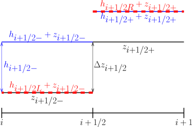
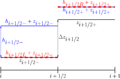
With (8), the defect of the hydrostatic reconstruction becomes apparent. To fix the ideas, suppose the local slope is positive, hence $\Delta z_{i+1/2}>0$, as in Figure 1. Then, for all $\Delta z_{i+1/2}$ such that $\Delta z_{i+1/2}\geq h_{i+1/2-}\geq 0$, the reconstruction gives $h_{i+1/2L}=0$, while $h_{i+1/2R}$ remains unchanged. In that case, the reconstruction prevents an unphysical negative value for $h_{i+1/2L}$, the counterpart of this being an underestimated difference $h_{i+1/2L}-h_{i+1/2R}$. Therefore, there is a lack in the numerical flux computed from the modified Riemann problem, which gives an underestimated velocity and consequently an overestimated height. This can be interpreted in terms of reconstructed slope as well, which is underestimated.

In the general case, we can write the following local criterion of “non validity” for the hydrostatic reconstruction.

Proposition 2.1

For a fixed discretization, if for some $i_{0}\leq i\leq i_{1}$ one has

$$\Delta z_{i+1/2}\geq h_{i+1/2-}\geq 0,\qquad\mbox{or}\quad-\Delta z_{i+1/2}\geq h_{i+1/2+}\geq 0,$$ (9)

then the hydrostatic reconstruction will overestimate (resp. underestimate) the water height (resp. velocity).

Notice that from a theoretical viewpoint, this is not limiting. Indeed, since this class of schemes is consistent with the system of partial differential equations (see [4]), the problem disappears when refining the discretization. However, it has to be taken into account for practical computations, with a fixed discretization. It is particularly apparent for order $1$ schemes, but also remains present for order $2$.

3 Numerical illustration

For numerical illustration purpose, we introduce an explicit solution which consists in a supercritical steady flow on an inclined plane with constant slope $\partial_{x}z=\alpha$ (it is referenced in the SWASHES library [8]). Steady states are solutions to

$$q(x,t)=q_{0}=Cst,\qquad\partial_{x}\left(hu^{2}+g\dfrac{h^{2}}{2}\right)=-gh\partial_{x}z,$$

and the height profile $h(x)$ must be a solution to Bernoulli’s law rewritten as a third order equation in $h$:

$$h^{3}+h^{2}\left(\alpha x-\dfrac{q_{0}^{2}}{2gh_{0}^{2}}-h_{0}\right)+\dfrac{q_{0}^{2}}{2g}=0,$$ (10)

where $h_{0}$ and $q_{0}=h_{0}u_{0}$ are the height and discharge at $x=0$, which completely determine the profile since the flow is supercritical. A careful study of the roots of the polynomial shows that the supercritical height profile is decreasing in $x$: $h(x)\leq h_{0}$ for all $x\geq 0$.

The numerical strategy we choose consists in the HLL flux and a modified MUSCL reconstruction. In [7], this combination of flux and linear reconstruction has shown to be the best compromise between accuracy, stability and CPU time cost. We refer to [4, 7] for a presentation of the HLL flux. The MUSCL reconstruction of a scalar function $s\in\mathbb{R}$ is

$$s_{i-1/2+}=s_{i}-\dfrac{\Delta x}{2}Ds_{i},\qquad s_{i+1/2-}=s_{i}+\dfrac{\Delta x}{2}Ds_{i},$$ (11)

where the “minmod” operator $D$ is given by

$$Ds_{i}=\text{minmod}\left(\dfrac{s_{i}-s_{i-1}}{\Delta x},\dfrac{s_{i+1}-s_{i}}{\Delta x}\right),\quad\text{minmod}(x,y)=\begin{cases}\min(x,y)&\text{if}\;x,y\geq 0,\\ \max(x,y)&\text{if}\;x,y\leq 0,\\ 0&\text{else.}\end{cases}$$ (12)

In order to keep the discharge conservation, the reconstruction of the velocity has to be modified as

$$u_{i-1/2+}=u_{i}-\dfrac{h_{i+1/2-}}{h_{i}}\dfrac{\Delta x}{2}Du_{i}\qquad u_{i+1/2-}=u_{i}+\dfrac{h_{i-1/2+}}{h_{i}}\dfrac{\Delta x}{2}Du_{i}.$$

Notice that if we take $Ds_{i}=0$ in (11), then $z_{i+1/2-}=z_{i+1/2-}=z_{i}$ so that the centered term (7) disappears, and we recover the first order scheme in space. Second order in time is achieved through a classical Heun predictor-corrector method.

We turn now to the specific data for simulations. The domain length is $L=10\;\text{m}$, and we choose initial data

$$h_{0}=h(x=0,t)=0.02\;\text{m},\qquad q_{0}=q(x=0,t)=0.01\;\text{m}^{2}/\text{s},$$

which is indeed supercritical. All simulations are performed with a space step $\Delta x=0.1\;\text{m}$, the time step is fixed in order to satisfy the CFL condition.

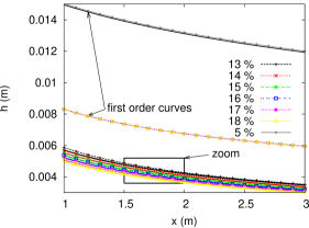
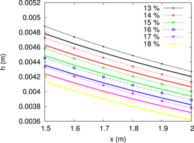
The analytical solution is computed with $7$ negative slopes $\alpha=5\%$, $13\%$, $14\%$, $15\%$, $16\%$, $17\%$ and $18\%$, both at first and second order. Numerical results are compared to the analytical results in Figure 2, where a part of the domain is displayed ($x$ between $1$ m and $3$ m).

With this set of data, a domain of admissible slopes can be estimated for the order $1$ hydrostatic reconstruction. Indeed since $\Delta z_{j+1/2}=|\alpha|\Delta x$, inserting a characteristic height of the flow $h^{*}$ in (9) gives a bound for the slope. One can use $h^{*}=h_{0}$, the incoming height. Since the height profile is decreasing, the whole profile will be wrong if $h_{0}\leq|\alpha|\Delta x$, that is here $|\alpha|\geq 20\%$. But actually, since the height decreases quite rapidly, a more accurate estimate is obtained for $x=1.5$ m with $h^{*}=0.005$ m (see Fig. 2), which leads to slopes above $5\%$.

We observe on Figure 2(Left) that with the first order scheme, the effect of the hydrostatic reconstruction is so important that all curves for slopes between $13\%$ and $18\%$ are superposed. In that case, the apparent result is the simulation of a single slope, namely $13\%$. For a $5\%$ slope, we still observe a slightly overestimated water height, as anticipated since $5\%$ is a limit case as observed above. With the second order, the water heights are still overestimated, but in a very slighter way, and the different curves are no longer identical (Figure 2(Right)).

Figure 2: Default of hydrostatic reconstruction: water height at first and second order of accuracy for different slopes. Dotted curves are simulations, plain curves are exact solutions. Left: first and second order curves. Right: zoom on second order curves

4 Conclusions

The hydrostatic reconstruction may fail for certain combinations of water height, slope and mesh size, namely in regions where (9) holds. The defaults are particularly apparent for order $1$ schemes, leading to wrongly estimated slopes, but still remain at order $2$, with some overestimated water heights. We emphasize that the problem disappears when refining the mesh, but has to be taken into account for a given discretization. The generalization of the hydrostatic reconstruction proposed in [6] does not exhibit the limitation discussed here, even for first order schemes, but positivity is not ensured. Other schemes involving threshold values (e.g. [5, 10]) very likely encounter the same kind of problem. Alternatively, the scheme recently introduced in [3] preserves the water height positivity and does not suffer from this problem. Notice finally that criterion (9) may be of some utility for adaptive mesh schemes, such as the ones used in Gerris [11].

References

- [1] E. Audusse, F. Bouchut, M.-O. Bristeau, R. Klein, B. Perthame. A fast and stable well-balanced scheme with hydrostatic reconstruction for shallow water flows. SIAM J. Sci. Comp., 25(6):2050–2065, 2004.
- [2] A. Bermudez, M.E. Vazquez. Upwind methods for hyperbolic conservation laws with source terms. Computers & Fluids, 23:1049–1071, 1994.
- [3] C. Berthon, F. Fouchet. Efficient well-balanced hydrostatic upwind schemes for shallow-water equations. J. Comput. Phys., 231(15):4993–5015, 2012.
- [4] F. Bouchut. Nonlinear stability of finite volume methods for hyperbolic conservation laws, and well-balanced schemes for sources. Frontiers in Mathematics, Birkhauser, 2004.
- [5] F. Bouchut, T. Morales. A subsonic-well-balanced reconstruction scheme for shallow water flows. SIAM J. Numer. Anal., 48(5):1733–1758, 2010.
- [6] M. Castro, A. Pardo, C. Parés. Well-balanced numerical schemes based on a generalized hydrostatic reconstruction technique. Math. Mod. Meth. App. Sci., 17(12):2055–2113,2007.
- [7] O. Delestre. Rain water overland flow on agricultural fields simulation/Simulation du ruissellement d’eau de pluie sur des surfaces agricoles. PhD thesis Université d’Orléans (French), 2010. tel.archives-ouvertes.fr/INSMI/tel-00531377/fr.
- [8] O. Delestre, C. Lucas, P.-A. Ksinant, F. Darboux, C. Laguerre, T.N.T. Vo, F. James and S. Cordier. SWASHES: a library of Shallow Water Analytic Solutions for Hydraulic and Environmental Studies. Accepted to Internt. J. Numer. Methods Fluids under minor revisions (July 2012).
- [9] J. M. Greenberg, A.-Y. Leroux. A well-balanced scheme for the numerical processing of source terms in hyperbolic equation. SIAM Journal on Numerical Analysis, 33:1–16, 1996.
- [10] Q. Liang, F. Marche. Numerical resolution of well-balanced shallow water equations with complex source terms. Advances in Water Resources, 32:873–884, 2009.
- [11] S. Popinet. Quadtree-adaptative tsunami modelling. Ocean Dynamics, 61(9):1261–1285, 2011.