SecDec: A tool for numerical multi-loop calculations

Abstract

The version 2.0 of the program SecDec is described, which can be used for the extraction of poles within dimensional regularisation from multi-loop integrals as well as phase space integrals. The numerical evaluation of the resulting finite functions is also done by the program in an automated way, with no restriction on the kinematics in the case of loop integrals.

1 Introduction

Nowadays we are in the long awaited situation of being confronted with a wealth of high energy collider physics data, enabling us to explore physics at the TeV scale. However, for the analysis and interpretation of these data, precise theory predictions are mandatory. In most cases, this means that calculations beyond the leading order in perturbation theory are necessary. Such calculations either involve integrations over loop momenta for the virtual corrections, or integrations over phase spaces for the real radiation corrections. In both cases, multi-dimensional parameter integrals need to be evaluated, which can contain ultraviolet singularities and, in the presence of massless particles, contain soft and/or collinear singularities. These singularities, if regulated by dimensional regularisation, appear as poles in $1/\epsilon$, but factorising the poles from complicated multi-loop or multi-parameter integrals is a highly non-trivial task. The program SecDec, presented in [1, 2], performs this task in an automated way, based on the algorithm of sector decomposition [3, 4, 5]. Other implementations of sector decomposition in public programs can be found in [6, 7, 8]. However, the latter programs, including SecDec 1.0 [1], are not designed to cope with kinematics where physical thresholds can be present in the integration region. The program SecDec 2.0 [2] is able to achieve this task, by an automated deformation of the integration contour into the complex plane [9, 10, 11, 12]. In this talk the emphasis is on the presentation of the new features of the program SecDec.

2 The algorithm

2.1 General framework

The decomposition algorithm is described in detail in [13], here we only describe the basic concepts. Consider an $N$-dimensional parameter integral, for example

$$I_{N}=\int_{0}^{1}dx_{1}\ldots\int_{0}^{1}dx_{N}\,x_{1}^{-1-\epsilon}\,\frac{g_{3}(\vec{x})}{\left[x_{1}\,g_{1}(\vec{x})+x_{2}\,g_{2}(\vec{x})\right]}\;,$$ (1)

where $g_{1},g_{2}$ are polynomial functions which do not vanish for $x_{1},x_{2}\to 0$. However, we would like to factorize the integrand such that the term in square brackets is non-vanishing in the limit $x_{1}\to 0,x_{2}\to 0$. This can be achieved by a decomposition into sectors where $x_{1}$ and $x_{2}$ are ordered: we multiply equation (1) with $1=\Theta(x_{1}-x_{2})+\Theta(x_{2}-x_{1})$ and substitute $x_{2}\to x_{1}\,x_{2}$ in the first sector and $x_{1}\to x_{2}\,x_{1}$ in the second sector, to arrive at

$$I_{N}=\int_{0}^{1}dx_{1}\ldots\int_{0}^{1}dx_{N}\,x_{1}^{-1-\epsilon}\,\left\{\frac{\tilde{g}_{3}}{\left[\tilde{g}_{1}(\vec{x})+x_{2}\,\tilde{g}_{2}(\vec{x})\right]}+x_{2}^{-1-\epsilon}\,\frac{\bar{g}_{3}}{\left[x_{1}\,\bar{g}_{1}(\vec{x})+\bar{g}_{2}(\vec{x})\right]}\right\}\;,$$ (2)

where $\tilde{g}_{i},\bar{g}_{i}$ are functions of the transformed variables. As $g_{1},g_{2}$ are non-vanishing at the origin, the terms in square brackets cannot lead to singularities anymore; the singularities are factored out into the monomials of type $x_{i}^{-1-\epsilon}$ instead, and subtraction of the poles and expansion in $\epsilon$ are straightforward in this form. In more complicated cases, the decomposition procedure may have to be iterated to achieve a full factorisation. A detailed description can be found e.g. in [3, 13].

2.2 Loop integrals

A scalar Feynman integral $G$ in $D$ dimensions at $L$ loops with $N$ propagators, where the propagators can have arbitrary, not necessarily integer powers $\nu_{j}$, has the following representation in momentum space:

$$G = \int\prod\limits_{l=1}^{L}{\mathrm{d}}^{D}\kappa_{l}\;\frac{1}{\prod\limits_{j=1}^{N}P_{j}^{\nu_{j}}(\{k\},\{p\},m_{j}^{2})}$$

$${\mathrm{d}}^{D}\kappa_{l} = \frac{\mu^{4-D}}{i\pi^{\frac{D}{2}}}\,{\mathrm{d}}^{D}k_{l}\;,\;P_{j}(\{k\},\{p\},m_{j}^{2})=q_{j}^{2}-m_{j}^{2}+i\delta\;,$$ (3)

where the $q_{j}$ are linear combinations of external momenta $p_{i}$ and loop momenta $k_{l}$. Introducing Feynman parameters leads to

$$G=\frac{(-1)^{N_{\nu}}}{\prod_{j=1}^{N}\Gamma(\nu_{j})}\Gamma(N_{\nu}-LD/2)\int\limits_{0}^{\infty}\,\prod\limits_{j=1}^{N}dx_{j}\,\,x_{j}^{\nu_{j}-1}\,\delta(1-\sum_{l=1}^{N}x_{l})\frac{{\cal U}^{N_{\nu}-(L+1)D/2}}{{\cal F}^{N_{\nu}-LD/2}}\,,\,N_{\nu}=\sum_{j=1}^{N}\nu_{j}\;,$$ (4)

where ${\cal U}$ is a polynomial of degree $L$ and ${\cal F}$ is of degree $L+1$ in the Feynman parameters. The Lorentz invariants which can be formed from the external momenta of the diagram, as well as propagator masses, are contained in ${\cal F}$. As a simple example, consider the function ${\cal F}$ for a massless one-loop box diagram:

$${\cal F}=-s_{12}\,x_{2}x_{4}-s_{23}\,x_{1}x_{3}-i\,\delta\;.$$ (5)

The functions ${\cal U}$ and ${\cal F}$ can also be constructed directly from the topology of the corresponding Feynman graph [14, 15], and the implementation of this construction in SecDec version 2.0 is one of the new features of the program.

For a diagram with massless propagators, none of the Feynman parameters occurs quadratically in the function ${\cal F}={\cal F}_{0}$ . If massive internal lines are present, ${\cal F}$ gets an additional term ${\cal F}(\vec{x})={\cal F}_{0}(\vec{x})+{\cal U}(\vec{x})\sum\limits_{j=1}^{N}x_{j}m_{j}^{2}$. ${\cal U}$ is a positive semi-definite function. A vanishing ${\cal U}$ function is related to the UV subdivergences of the graph. In the region where all invariants formed from external momenta are negative, which we will call the Euclidean region in the following, ${\cal F}$ is also a positive semi-definite function. Its vanishing does not necessarily lead to an IR singularity. Only if some of the invariants are zero, for example if some of the external momenta are light-like, the vanishing of ${\cal F}$ may induce an IR divergence. Thus it depends on the kinematics and not only on the topology (like in the UV case) whether a zero of ${\cal F}$ leads to a divergence or not. The necessary (but not sufficient) conditions for a divergence are given by the Landau equations [16]:

$$x_{j}\,(q_{j}^{2}-m_{j}^{2})=0\quad\forall\,j$$ (6)

$$\frac{\partial}{\partial k_{l}^{\mu}}\sum_{j}x_{j}\,\left(q_{j}^{2}(k,p)-m_{j}^{2}\right)=0\;.$$ (7)

If all kinematic invariants formed by external momenta are of the same sign, the necessary condition ${\cal F}=0$ for an IR divergence can only be fulfilled if some of the parameters $x_{i}$ go to zero. These singularities can be regulated by dimensional regularisation and factored out of the function ${\cal F}$ using sector decomposition. The same holds for dimensionally regulated UV singularities contained in ${\cal U}$. However, after these singularities, appearing as poles in 1/$\epsilon$, have been extracted using sector decomposition, for non-Euclidean kinematics we are still faced with integrable singularities related to kinematic thresholds. How we deal with these singularities will be described in Section 4.4.

2.3 General parameter integrals

The program can also deal with parameter integrals which are more general than the ones related to multi-loop integrals, for example phase space integrals involving massless particles, where the regions in phase space corresponding to soft and/or collinear configurations lead to singularities which can be extracted as poles in $1/\epsilon$. The only restrictions are that the integration domain should be the unit hypercube, and the singularities should be only endpoint singularities, i.e. should be located at zero or one. We assume that the singularities are regulated by non-integer powers of the integration parameters, where the non-integer part is the $\epsilon$ of dimensional regularisation or some other regulator. The general form of the integrals is

$$I=\int_{0}^{1}dx_{1}\ldots\int_{0}^{1}dx_{N}\prod_{i=1}^{m}P_{i}(\vec{x},\{\alpha\})^{\nu_{i}}\;,$$ (8)

where $P_{i}(\vec{x},\{\alpha\})$ are polynomial functions of the parameters $x_{j}$, which can also contain some symbolic constants $\{\alpha\}$. The user can leave the parameters $\{\alpha\}$ symbolic during the decomposition, specifying numerical values only for the numerical integration step. This way the decomposition and subtraction steps do not have to be redone if the values for the constants are changed. The $\nu_{i}$ are powers of the form $\nu_{i}=a_{i}+b_{i}\epsilon$ (with $a_{i}$ such that the integral is convergent). Note that half integer powers are also possible.

3 The SecDec program

The program consists of two parts, an algebraic part and a numerical part. The algebraic part uses code written in Mathematica [17] and does the decomposition into sectors, the subtraction of the singularities, the expansion in $\epsilon$ and the generation of the files necessary for the numerical integration. In the numerical part, Fortran or C++ functions forming the coefficient of each term in the Laurent series in $\epsilon$ are integrated using the Monte Carlo integration programs contained in the Cuba library [18, 19], or Bases [20]. The different subtasks are handled by perl scripts. The flowchart of the program is shown in Fig. 1 for the basic flow of input/output streams.

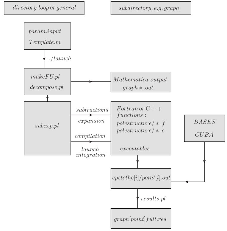
Figure 1: Flowchart showing the main steps the program performs to produce the result files. In each of the subdirectories loop or general, the file Template.m can be used to define the integrand. The produced files are written to a subdirectory created according to the settings given in param.input. By default, a subdirectory with the name of the graph or integrand is created to store the produced functions. This directory will contain subdirectories according to the pole structure of the integrand.

The directories loop and general have the same global structure, only some of the individual files are specific to loops or to more general parametric functions. The directories contain a number of perl scripts steering the decomposition and the numerical integration. The scripts use perl modules contained in the subdirectory perlsrc.

The Mathematica source files are located in the subdirectories src/deco (files used for the decomposition), src/subexp (files used for the pole subtraction and expansion in $\epsilon$) and src/util (miscellaneous useful functions). The documentation, created by robodoc [21] is contained in the subdirectory doc. It contains an index to look up documentation of the source code in html format by loading masterindex.html into a browser.

In order to use the program, the user only has to edit the following two files:

• param.input: (text file)
  specification of paths, type of integrand, order in $\epsilon$, output format, parameters for numerical integration, further options

• Template.m: (Mathematica syntax)

  • for loop integrals: specification of loop momenta and propagators, resp. of the topology; optionally numerator, non-standard propagator powers, space-time dimensions

  • for general functions: specification of integration variables, integrand, variables to be split

The program comes with example input and template files in the subdiretories loop/demos respectively general/demos, described in detail in [1].

4 Installation and usage

4.1 Installation

The program can be downloaded from
http://projects.hepforge.org/secdec.

Unpacking the tar archive via tar xzvf SecDec.tar.gz will create a directory called SecDec with the subdirectories as described above. Then change to the SecDec directory and run ./install.

Prerequisites are Mathematica, version 6 or above, perl (installed by default on most Unix/Linux systems), a Fortran compiler (e.g. gfortran, ifort), or a C++ compiler if the C++ option is used.

4.2 Usage

1. Change to the subdirectory loop or general, depending on whether you would like to calculate a loop integral or a more general parameter integral.

2. Copy the files param.input and Template.m to create your own parameter and template files myparamfile, mytemplatefile.

3. Set the desired parameters in myparamfile and specify the integrand in mytemplatefile.

4. Execute the command ./launch -p myparamfile -t mytemplatefile in the shell.
   If you omit the option -p myparamfile, the file param.input will be taken as default. Likewise, if you omit the option -t mytemplatefile, the file Template.m will be taken as default. If your files myparamfile, mytemplatefile are in a different directory, say, myworkingdir, use the option -d myworkingdir, i.e. the full command then looks like ./launch -d myworkingdir -p myparamfile -t mytemplatefile, executed from the directory SecDec/loop or SecDec/general.
   

5. Collect the results. Depending on whether you have used a single machine or submitted the jobs to a cluster, the following actions will be performed:

   • If the calculations are done sequentially on a single machine, the results will be collected automatically (via results.pl called by launch). The output file will be displayed with your specified text editor.

   • If the jobs have been submitted to a cluster, when all jobs have finished, execute the command ./results.pl [-d myworkingdir -p myparamfile]. This will create the files containing the final results in the graph subdirectory specified in the input file.

6. After the calculation and the collection of the results is completed, you can use the shell command ./launchclean[graph] to remove obsolete files.

It should be mentioned that the code starts working first on the most complicated pole structure, which takes longest. This is because in case the jobs are sent to a cluster, it is advantageous to first submit the jobs which are expected to take longest.

4.3 New features

Version 2.0 of SecDec contains the following new features, some of which will be illustrated by examples in Section 5. More details are given in [2].

• Multi-scale loop integrals can be evaluated without restricting the kinematics to the Euclidean region.

• The possibility to loop over ranges of parameter values is automated, with the option of outputting results in a format suitable for plotting.

• The user can define functions at a symbolic level and specify them only later after the integrand has been transformed into a set of finite functions for each order in $\epsilon$.

• The regulator of the parameter integrals can be different from the dimensional regulator $\epsilon$. This is particularly useful to define e.g. measurement functions at a later stage of the calculation.

• For scalar multi-loop integrals, the integrand can be constructed directly from the topology of the diagram. The user only has to provide the labels of the vertices connected by the propagators and the propagator masses, but does not have to provide the momentum flow.

• The files for the numerical integration of multi-scale loop integrals are written in C++ rather than Fortran. For integrations in Euclidean space, both the Fortran and the C++ versions are supported.

• Both the algebraic and the numerical part allow full parallelisation.

4.4 Implementation of the contour deformation

Unless the function ${\cal F}$ in equation (4) is of definite sign for all possible values of invariants and Feynman parameters, the integrand of a multi-loop integral will vanish within the integration region on a hypersurface given by the solutions of the Landau equations (6),(7). However, we can avoid the poles on the real axis by a deformation of the integration contour into the complex plane. As long as the deformation is in accordance with the causal $i\delta$ prescription of the Feynman propagators, and no poles are crossed while changing the integration path, we can make use of Cauchy’s theorem to choose an integration contour such that the integration is convergent. The $i\delta$ prescription for the Feynman propagators tells us that the contour deformation into the complex plane should be such that the imaginary part of ${\cal F}$ should always be negative. For real masses and Mandelstam invariants $s_{ij}$, the following Ansatz [9, 10, 11, 12] is convenient:

$$\vec{z}(\vec{x}) = \vec{x}-i\;\vec{\tau}(\vec{x})\;,$$

$$\tau_{k} = \lambda\,x_{k}(1-x_{k})\sum\limits_{j=1}^{N-1}\,\frac{\partial{\cal F}}{\partial x_{j}}\;.$$ (9)

In terms of the new variables, we thus obtain

$${\cal F}(\vec{z}(\vec{x}))={\cal F}(\vec{x})-i\,\lambda\,\sum\limits_{j=1}^{N-1}\,\left(\frac{\partial{\cal F}}{\partial x_{j}}\right)^{2}+{\cal O}(\lambda^{2})\;,$$ (10)

such that ${\cal F}$ acquires a negative imaginary part of order $\lambda$.

The convergence of the numerical integration can be improved significantly by choosing an “optimal” value for $\lambda$. Values of $\lambda$ which are too small lead to contours which are too close to the poles on the real axis and therefore lead to bad convergence. Too large values of $\lambda$ can modify the real part of the function to an unacceptable extent and could even change the sign of the imaginary part if the terms of order $\lambda^{3}$ get larger than the terms linear in $\lambda$. This would lead to a wrong result. Therefore we implemented a four-step procedure to optimize the value of $\lambda$, consisting of

• ratio check: To make sure that the terms of order $\lambda^{3}$ in equation (10) do not spoil the sign of the imaginary part, we evaluate the ratio of the terms linear and cubic in $\lambda$ for a quasi-randomly chosen set of sample points to determine a maximal allowed $\lambda=\lambda_{max}$.

• modulus check: The imaginary part is vital at the points where the real part of ${\cal F}$ is vanishing. In these regions, the deformation should be large enough to avoid large numerical fluctuations due to a highly peaked integrand. Therefore we check the modulus of each subsector function ${\cal F}_{i}$ at a number of sample points, and pick the fraction of the value of $\lambda_{max}$ maximising the function with the minimal modulus, i.e. the value of lambda which keeps $\mathcal{F}$ furthest from zero.

• individual $\lambda(i,j)$ adjustments: If the values of $\frac{\partial{\cal F}_{i}}{\partial x_{j}}$ are very different in magnitude, it can be convenient to have an individual parameter $\lambda(i,j)$ for each subsector function ${\cal F}_{i}$ and each Feynman parameter $x_{j}$.

• sign check: After the above adjustments to $\lambda$ have been made, the sign of Im$(\mathcal{F})$ is again checked for a number of sample points. If the sign is ever positive, this value of $\lambda$ is disallowed.

5 Examples and results

In this example, we will demonstrate three of the new features of the SecDec 2.0 program: the construction of $\mathcal{F},\mathcal{U}$ directly from the topology of the graph, the evaluation of the graph in the physical region, and how results for a whole set of different numerical values for the invariants can be produced and plotted in an automated way. We will use the two-loop diagram shown in Fig. 2 as an example. Numerical results for this diagram have been produced in [22, 23], analytical ones in [24, 25].

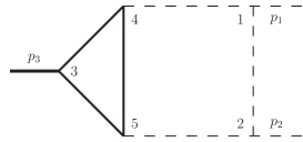
Figure 2: Two-loop vertex graph called $P_{126}$, containing a massive triangle loop. Bold lines are massive, dashed lines are massless. The vertices are labeled to match the construction of the integrand from the topology as explained in the text.

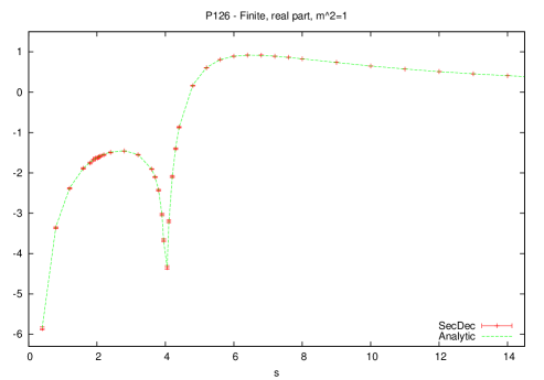
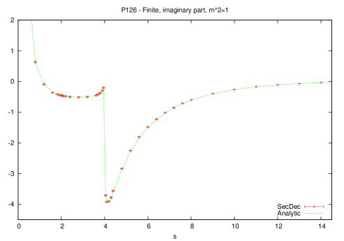
Figure 3: Comparison of analytic and numerical results for the diagram $P_{126}$.

5.1 Topology-based construction of the integrand

The template file templateP126.m in the demos subdirectory contains the following lines:
$proplist=\{\{ms[1],\{3,4\}\},\{ms[1],\{4,5\}\},\{ms[1],\{5,3\}\},\{0,\{1,2\}\},\{0,\{1,4\}\},\{0,\{2,5\}\}\};$
$onshell=\{ssp[1]\to 0,ssp[2]\to 0,ssp[3]\to sp[1,2]\};$
where each entry in $proplist$ corresponds to a propagator of the diagram; the first entry is the mass of the propagator, and the second entry contains the labels of the two vertices which the propagator connects. Note that if an external momentum $p_{k}$ is flowing into the vertex, the vertex also must have the label $k$. For vertices containing only internal propagators the labeling is arbitrary. The on-shell conditions in the above example state that $p_{1}^{2}=p_{2}^{2}=0,\,p_{3}^{2}=s$.

5.2 Results in the physical region

To run this example, from the loop directory, issue the command ./launch -d demos -p paramP126.input -t templateP126.m. The timings for the finite part and a relative accuracy better than 1%, using Cuba-3.0 [19], are about 100 seconds per point on an Intel(R) Core i7 CPU at 2.67GHz, where the timings are very similar far from the $s=4m^{2}$ threshold and close to threshold.

5.3 Producing data files for sets of numerical values

To loop over a set of numerical values for the invariants $s$ and $m^{2}$ once the C++ files are created, issue the command
./multinumerics.pl -d demos -p multiparamP126.input. This will run the numerical integrations for the values of $s$ and $m^{2}$ specified in the file demos/multiparamP126.input. The files containing the results will be found in demos/2loop/P126, and the files p-2.gpdat, p-1.gpdat and p0.gpdat will contain the data files for each point, corresponding to the coefficients of $\epsilon^{-2},\epsilon^{-1}$ and $\epsilon^{0}$ respectively. These files can be used to plot the results against the analytic results using gnuplot. This will produce the files P126R0.ps, P126I0.ps which will look like Fig. 3.

6 Conclusions

We have presented the program SecDec 2.0, which can be used to factorise dimensionally regulated singularities and numerically calculate multi-loop integrals in an automated way. As a new feature of the program, it now can deal with physical kinematics, i.e. is not restricted to the Euclidean region anymore. A new construction of the integrand, based entirely on topological rules, is also included, and the new features are demonstrated for the examples of a massive two-loop three-point function. In addition, the program can produce numerical results for more general parameter integrals, as they occur for example in phase space integrals for multi-particle production with several unresolved massless particles, and offers the possibility to include symbolic functions which can be used to define measurement functions like e.g. jet algorithms at a later stage. We are looking forward to applications of the program for the calculation of higher order corrections to various observables.

References

References

- [1] Carter J and Heinrich G 2011 Comput.Phys.Commun. 182 1566–1581 (Preprint 1011.5493)
- [2] Borowka S, Carter J and Heinrich G 2012 (Preprint 1204.4152)
- [3] Binoth T and Heinrich G 2000 Nucl. Phys. B585 741–759 (Preprint hep-ph/0004013)
- [4] Roth M and Denner A 1996 Nucl. Phys. B479 495–514 (Preprint hep-ph/9605420)
- [5] Hepp K 1966 Commun. Math. Phys. 2 301–326
- [6] Smirnov A, Smirnov V and Tentyukov M 2011 Comput.Phys.Commun. 182 790–803 (Preprint 0912.0158)
- [7] Bogner C and Weinzierl S 2008 Comput. Phys. Commun. 178 596–610 (Preprint 0709.4092)
- [8] Gluza J, Kajda K, Riemann T and Yundin V 2011 Eur.Phys.J. C71 1516 (Preprint 1010.1667)
- [9] Soper D E 2000 Phys. Rev. D62 014009 (Preprint hep-ph/9910292)
- [10] Nagy Z and Soper D E 2006 Phys. Rev. D74 093006 (Preprint hep-ph/0610028)
- [11] Binoth T, Guillet J P, Heinrich G, Pilon E and Schubert C 2005 JHEP 10 015 (Preprint hep-ph/0504267)
- [12] Anastasiou C, Beerli S and Daleo A 2007 JHEP 05 071 (Preprint hep-ph/0703282)
- [13] Heinrich G 2008 Int. J. Mod. Phys. A23 1457–1486 (Preprint 0803.4177)
- [14] Nakanishi N 1971 Graph Theory and Feynman Integrals (Gordon and Breach, New York)
- [15] Tarasov O V 1996 Phys. Rev. D54 6479–6490 (Preprint hep-th/9606018)
- [16] Landau L D 1959 Nucl. Phys. 13 181–192
- [17] Wolfram S , Mathematica, Copyright by Wolfram Research
- [18] Hahn T 2005 Comput. Phys. Commun. 168 78–95 (Preprint hep-ph/0404043)
- [19] Agrawal S, Hahn T and Mirabella E 2011 (Preprint 1112.0124)
- [20] Kawabata S 1995 Comp. Phys. Commun. 88 309–326
- [21] Slothouber F and et al http://www.xs4all.nl/ rfsber/Robo/robodoc.html
- [22] Bonciani R, Mastrolia P and Remiddi E 2004 Nucl.Phys. B690 138–176 (Preprint hep-ph/0311145)
- [23] Ferroglia A, Passera M, Passarino G and Uccirati S 2004 Nucl.Phys. B680 199–270 (Preprint hep-ph/0311186)
- [24] Fleischer J, Kotikov A and Veretin O 1998 Phys.Lett. B417 163–172 (Preprint hep-ph/9707492)
- [25] Davydychev A I and Kalmykov M 2004 Nucl.Phys. B699 3–64 (Preprint hep-th/0303162)