Simulations of the kinematic dynamo onset of spherical Couette flows with smooth and rough boundaries

Abstract

We study numerically the dynamo transition of an incompressible electrically conducting fluid filling the gap between two concentric spheres. In a first series of simulations, the fluid is driven by the rotation of a smooth inner sphere through no-slip boundary conditions, whereas the outer sphere is stationary. In a second series a volume force intended to simulate a rough surface drives the fluid next to the inner sphere within a layer of thickness one tenth of the gap width. We investigate the effect of the boundary layer thickness on the dynamo threshold in the turbulent regime. The simulations show that the boundary forcing simulating the rough surface lowers the necessary rotation rate, which may help to improve spherical dynamo experiments.

I Introduction

Dynamo theory describes the generation of magnetic fields in flows of conducting fluids, for example in stars or planetary interiors. Several experiments have been built in order to reproduce a dynamo in the laboratory. After the first experiments in Riga Gailitis et al. (2000) and Karlsruhe Muller and Stieglitz (2002), more recent experiments Monchaux et al. (2007); Lathrop and Forest (2011) implement flows less confined to specific shapes than the first experiments, so that the effect of turbulence on dynamo action is more relevant. Nevertheless, the main contribution to magnetic field generation in these experiments is still assumed to come from the time averaged part of the flows. The numerical investigations presented in this paper are directly applicable to spherical experiments like those in Maryland Lathrop and Forest (2011).

The spherical Couette flow with a stationary outer sphere is mainly a differential rotation driven by the inner sphere, together with a jet in the equatorial plane in which fluid is centrifuged radially outward. A flow along the rotation axis connecting the poles of the two spheres brings the fluid back to the inner sphere. The flow thus consists of differential rotation and two loops in the meridional circulation. It is helical with opposite helicities in the two hemispheres and is topologically equivalent to the s2t1 flows studied by Dudley and James Dudley and James (1989) which are known to be dynamos. The spherical Couette flow on the contrary does not generate magnetic fields for Reynolds numbers $\mathrm{Re}$ up to a critical value where the flow becomes unstable Guervilly and Cardin (2010). It therefore seems possible that turbulent spherical Couette flow is a small scale dynamo. In this type of dynamos, at magnetic Prandtl numbers $\mathrm{Pm}$ with $\mathrm{Pm}\gg 1$, the largest production of the magnetic field occurs at the resistive scale and the critical magnetic Reynolds number $\mathrm{Rm}$ increases with increasing hydrodynamic Reynolds number. For $\mathrm{Pm}\ll 1$, the largest production of magnetic field occurs at some scale larger than the viscous scale Schekochihin et al. (2004); Iskakov et al. (2007), so that the critical $\mathrm{Rm}$ is independent of $\mathrm{Re}$ for $\mathrm{Re}$ large enough, because increasing $\mathrm{Re}$ then adds small vortices with magnetic Reynolds numbers less than 1. The magnetic field shows nothing but diffusive dynamics on these length scales so that they do not contribute to either creation or mixing of magnetic field. Ref. Guervilly and Cardin, 2010 found $\mathrm{Rm_{c}}$ to increase with $\mathrm{Re}$ for the entire investigated parameter range, which further adds to the suspicion that spherical Couette flows could be small scale dynamos. Since the Reynolds number $\mathrm{Re}$ in numerical simulations is limited, the magnetic Prandtl number $\mathrm{Pm}$ has to be adjusted to values far above the $\mathrm{Pm}$ of liquid sodium (which is the liquid commonly used in experiments) in order to achieve high enough magnetic Reynolds numbers. There is always a need to extrapolate from numerical results to larger $\mathrm{Re}$, so that it is always important to understand the dependence of the dynamo threshold on $\mathrm{Re}$ and $\mathrm{Pm}$ Schekochihin et al. (2004); Iskakov et al. (2007); Ponty et al. (2005).

An experiment is under construction which realizes spherical Couette flow in liquid metals Triana (2011). One motivation for the present study is to predict whether this experiment will be able to sustain a self-generated magnetic field. This question will be investigated in section III. Because of the pessimistic answer obtained in this section, section IV considers the possible improvement obtained by welding blades on the inner sphere in order to strengthen the coupling between the fluid and the rotation of the inner sphere.

II The mathematical model

The system under investigation consists of two concentric speres with radii $R_{i}$ and $R_{o}$ forming a gap of width $R_{i}-R_{o}=d$ and aspect ratio $R_{i}/R_{o}=1/3$. The fluid in the gap is driven by the rotation of the inner core, which rotates at angular frequency $\Omega_{i}$ about the $z-$axis, while the outer boundary is at rest. The fluid is characterized by its kinematic viscosity $\nu$ and its magnetic diffusivity $\lambda$. The evolution of the magnetic field in an incompressible electrically conducting fluid is described by the induction equation. The system is governed by two numbers, the Reynolds number $\mathrm{Re}$, and the magnetic Prandtl number $\mathrm{Pm}$ or alternatively the magnetic Reynolds number $\mathrm{Rm}$ defined by

$$\mathrm{Re}=\frac{\Omega_{i}d^{2}}{\nu},\qquad\mathrm{Pm}=\frac{\nu}{\lambda},\qquad\mathrm{Rm}=\mathrm{Re}\text{ }\mathrm{Pm}.$$ (1)

From now on, only adimensional variables will be used in this paper. Choosing as units of time and length the reciprocal of the inner core’s rotation rate and the gap width, the induction equation reads for non-dimensional magnetic and velocity fields $\bm{B}$ and $\bm{v}$:

$$\partial_{t}\bm{B}+\nabla\times(\bm{B}\times\bm{v})=\frac{1}{\mathrm{Re}\text{ }\mathrm{Pm}}\nabla^{2}\bm{B}~{}~{}~{},~{}~{}~{}\nabla\cdot\bm{B}=0.$$ (2)

The velocity field itself is a solenoidal vector field determined by the Navier-Stokes equation and the continuity equation:

$$\partial_{t}\bm{v}+(\bm{v}\cdot\nabla)\bm{v}=-\nabla\Phi+\frac{1}{\mathrm{Re}}\nabla^{2}\bm{v}\text{ }+\bm{F}~{}~{}~{},~{}~{}~{}\nabla\cdot\bm{v}=0.$$ (3)

Eq. (3) contains a volume force $\bm{F}$ and $\Phi$ stands for the pressure variable. Eqs. (2) and (3) describe the kinematic dynamo problem, in which one assumes the system to be near the onset of magnetic field generation, so that the magnetic field strength is small and the Lorentz force is negligible in equation (3).

The parameters $\mathrm{Re}$ and $\mathrm{Rm}$ depend on the inner core’s rotation rate. More revealing parameters are the Reynolds numbers $\mathrm{\overline{Re}}$ and $\mathrm{\overline{Rm}}$ based on the rms velocity $\overline{v_{\text{rms}}}$ defined as

$$\overline{v_{\text{rms}}}=\sqrt{2E_{\mathrm{kin}}/V}~{}~{}~{},~{}~{}~{}E_{\mathrm{kin}}=\langle\int\frac{1}{2}\bm{v}^{2}dV\rangle$$ (4)

and

$$\mathrm{\overline{Re}}=\mathrm{Re}\text{ }\overline{v_{\text{rms}}}~{}~{}~{},~{}~{}~{}\mathrm{\overline{Rm}}=\mathrm{\overline{Re}}\text{ }\mathrm{Pm}$$ (5)

where $V$ is the volume of the shell, brackets denote time average and $E_{\mathrm{kin}}$ the kinetic energy.

In the following the effect of different surface properties on the dynamo threshold are compared. The inner and outer spheres have radii $r_{i}=1/2$ and $r_{o}=3/2$, respectively. The inner sphere and the space surrounding the outer sphere are assumed to be insulating. Two different types of boundary forcing are implemented in order to simulate both smooth and rough surfaces. For the smooth surface no-slip boundary conditions

$$\bm{v}=\hat{\bm{z}}\times\bm{r}~{}~{}~{}\mbox{at}~{}~{}~{}r=r_{i}~{}~{}~{},~{}~{}~{}\bm{v}=0~{}~{}~{}\mbox{at}~{}~{}~{}r=r_{o}$$ (6)

are chosen together with $\bm{F}=0$ in eq. (3). In the second case, the inner boundary is assumed free slip and the fluid is driven in one tenth of the gap width by a toroidal force field $\bm{F}$ of spherical harmonic degree $l=1$ and order $m=0$, given in spherical polar coordinates $(r,\theta,\varphi)$ by:

$$\bm{F}=\frac{1}{2}\left[1-\tanh\left(\frac{60}{d}(r-r_{i}-\frac{d}{10})\right)\right]\sin\theta\text{ }\hat{e}_{\varphi}.$$ (7)

This forcing qualitatively reproduces the flow driven by an inner sphere with blades of height one tenth the gap size mounted along meridians. The non-dimensional rotation rate of the inner sphere, $\Omega^{\prime}_{i}$, has to be found a posteriori in these simulations by computing

$$\Omega^{\prime}_{i}=\frac{3}{8\pi r_{i}}\int_{0}^{2\pi}d\varphi\int_{0}^{\pi}d\theta~{}\sin^{2}\theta\langle v_{\varphi}(r=r_{i},\theta,\varphi,t)\rangle$$ (8)

with which a Reynolds number $\mathrm{Re^{\prime}}$, analogous to $\mathrm{Re}$ for the no slip boundaries, is defined as

$$\mathrm{Re^{\prime}}=\mathrm{Re}\text{ }\Omega^{\prime}_{i}$$ (9)

In the following $\mathrm{Re}$ is going to be increased up to $1.67\cdot 10^{4}$ for the no-slip boundary conditions and up to $2.5\cdot 10^{3}$ in the simulations utilizing the volume force. The magnetic Prandtl number is of order unity for the simulations just at the onset of magnetic amplification. The numerical method is a spectral method, in which the fields are expanded in spherical harmonics and Chebychev polynomials Tilgner (1999).

III No-slip

III.1 Hydrodynamic Characteristics

The hydrodynamic properties of the spherical Couette flow with stationary outer sphere have already been investigated in detail in Dumas and Leonard (1994); Hollerbach et al. (2006); Guervilly and Cardin (2010). At low Reynolds numbers the basic spherical Couette flow is axisymmetric and we find a critical Reynolds number of $\mathrm{Re_{h}}=1500$ ($\mathrm{\overline{Re}_{h}}=105$) beyond which small non-axisymmetric perturbations increase and an instability develops as a propagating wave on the equatorial jet with a dominant azimuthal wavenumber $m=2$, which is in agreement with Guervilly and Cardin (2010); Hollerbach et al. (2006). At $\mathrm{Re_{s}}=2800$ ($\mathrm{\overline{Re}_{s}}=178$) a second transition occurs. Beyond this value, the amplitudes of odd wavenumbers $m$ of the kinetic energy develop as well and the power spectrum begins to flatten and approaches power laws in $m^{-5/3}$ and $l^{-5/3}$, indicative of Kolmogorov turbulence (see Figure 1). Large scales of the velocity field, however, have comparable spectra for all $\mathrm{Re}$. The bottom panel shows the power spectra of an estimate of the turbulent rate of strain of spherical harmonic order l, which is simply the kinetic energy multiplied by $l^{2}$ and has its maximum at the viscous scale. At $\mathrm{\overline{Re}}=970$ the inertial range reaches up to $l\approx 40$.

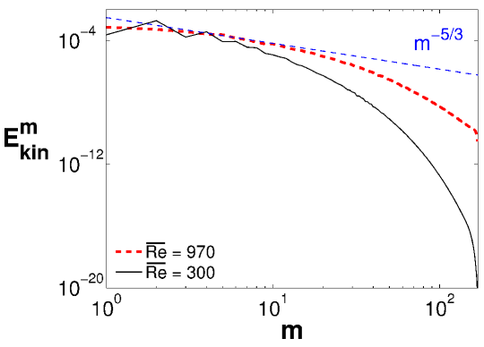
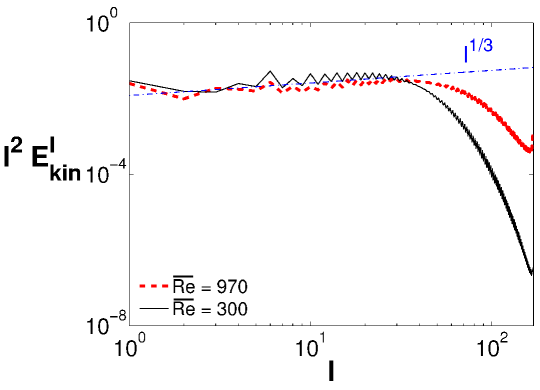
Figure 1: (Color online) Power spectrum of kinetic energy plotted against spherical harmonic degree $m$ (top) and the turbulent rate of strain versus spherical harmonic order $l$ (bottom) for $\mathrm{\overline{Re}}=300$ (black continuous line) and $970$ (thick red dashed line), together with the Kolmogorov power laws $m^{-5/3}$ and $l^{1/3}$ (blue dashed line).

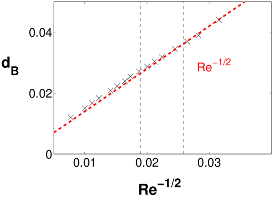
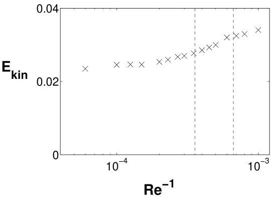
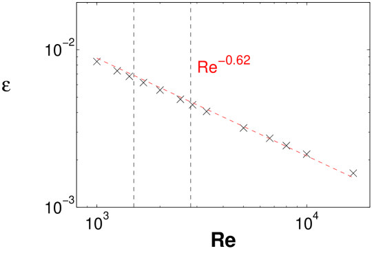
Figure 2: (Color online) Boundary layer thickness $d_{B}$ plotted against $\mathrm{Re}^{-1/2}$ (top), kinetic energy plotted against $\mathrm{Re}^{-1}$ (middle), and energy dissipation rate plotted against $\mathrm{Re}$ (bottom). The vertical dashed lines mark $\mathrm{Re_{h}}$ and $\mathrm{Re_{s}}$.

The wavenumber of the most unstable mode depends on the aspect ratio of the shell and switches from $m=2$ to $m=3$ at an aspect ratio close to the one chosen here Hollerbach et al. (2006). It is possible to generate flows with $m=3$ as dominating mode by starting from an equilibrated solution at $\mathrm{Re}>\mathrm{Re_{s}}$ and lowering $\mathrm{Re}$ to some value in between $\mathrm{Re_{h}}$ and $\mathrm{Re_{s}}$.

Figure 2 (top) shows the thickness of the boundary layer of $u_{\varphi}$ near the inner core. In order to produce this figure, $u_{\varphi}$ has been averaged over spherical surfaces and the boundary layer thickness defined as the distance from the inner sphere at which this averaged velocity drops to the arithmetic mean of its value at the boundary and its value averaged over radius. At high $\mathrm{Re}$ the evolution of the boundary layer thickness is approaching $\mathrm{Re}^{-1/2}$, as one would expect from theory.

Figure 2 (middle) shows the dependence of the dimensionless kinetic energy on $\mathrm{Re}$, which converges to a constant in the limit of $\mathrm{Re}^{-1}\rightarrow 0$. The viscosity becomes irrelevant for high $\mathrm{Re}$ and the only remaining control parameters entering the dimensional kinetic energy are the density and $\mathrm{\Omega_{i}}$, so that the kinetic energy scales with $\Omega_{i}^{2}$ and the dimensionless kinetic energy becomes constant.

A quantity of direct relevance to experiments is the energy dissipated in the flow. The energy budget, obtained by taking the scalar product of eq. (3) with $\bm{v}$ and integrating over space, reads

$$\partial_{t}\int\frac{1}{2}\bm{v}^{2}dV=\frac{1}{\mathrm{Re}}\tau-\frac{1}{\mathrm{Re}}\int(\partial_{i}v_{j})^{2}dV+\int\bm{F}\cdot\bm{v}dV$$ (10)

with

$$\tau=-\int_{0}^{2\pi}d\varphi\int_{0}^{\pi}d\theta r^{3}\sin^{2}\theta\left(\partial_{r}v_{\varphi}-\frac{v_{\varphi}}{r}\right),$$ (11)

evaluated on the inner boundary $r=r_{i}$, being the torque on the inner boundary. $\bm{F}=0$ for the simulations in this section so that the time averaged torque $\langle\tau\rangle$ is directly related to the energy dissipation $\epsilon$ by $\epsilon=\langle\tau\rangle/\mathrm{Re}$. As shown in fig. 2, the dissipation scales as $\mathrm{Re}^{-0.62}$. The bracket in the integrand in eq. (11) is dominated by the derivative $\partial_{r}v_{\varphi}$ which can be estimated as $v_{\mathrm{rel}}/d_{B}$, where $d_{B}$ is the boundary layer thickness and $v_{\mathrm{rel}}$ the velocity of the inner boundary relative to the bulk fluid. Since $d_{B}\propto\mathrm{Re}^{-1/2}$, we have $\epsilon\propto\mathrm{Re}^{-1/2}v_{\mathrm{rel}}$. If the motion of the inner core was completely decoupled from the rotation of the inner boundary, $v_{\mathrm{rel}}$ would be independent of $\mathrm{Re}$ and $\epsilon\propto\mathrm{Re}^{-1/2}$. There is of course some entrainment of the fluid by the rotation rate of the inner sphere and one finds an exponent of -0.62 instead of -0.5.

III.2 Dynamo transition

The dynamo transition for the spherical Couette flow with stationary outer sphere has already been computed in Guervilly and Cardin (2010) with different magnetic boundary conditions and an aspect ratio of $r_{i}/r_{o}=0.35$. These results will be compared with ours in the last section. Figure 3 shows the dynamo simulations in the $(\mathrm{\overline{Re}},\mathrm{\overline{Rm}})-$plane. Asterisks mark working dynamos and dots are failed dynamos. Linear interpolation between the growth rates computed at those points allows us to find the locus of zero growth rate. The onset of magnetic field amplification obtained in this way is indicated by the dashed line. The magnetic fields are dominated by modes with an azimuthal wavenumber of $m=2$. As mentioned above, suitable initial conditions lead to magnetic fields dominated by modes with $m=3$. The onset for these dynamos is indicated by the thick solid line. The two lines coincide for $\mathrm{\overline{Re}}>\mathrm{\overline{Re}_{s}}$. The straight line indicates $\mathrm{Pm}=1$. Except for the highest $\mathrm{\overline{Re}}$ the magnetic Prandtl number is always larger than one. In agreement with Guervilly and Cardin (2010) there are no working dynamos for axisymmetric flows. For $\mathrm{\overline{Re}_{h}}<\mathrm{\overline{Re}}<\mathrm{\overline{Re}_{s}}$ the critical magnetic Reynolds number $\mathrm{\overline{Rm}_{c}}$ for $m=2$ first increases, reaches a maximum and finally decreases, until at the second transition odd modes of the kinetic energy become unstable and the dynamo threshold again increases.

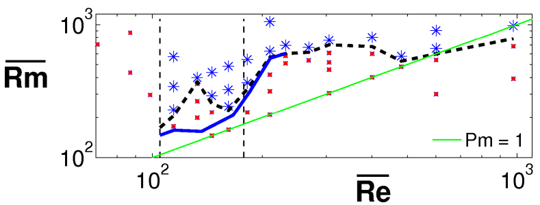
Figure 3: (Color online) Dynamo transition for magnetic fields dominated by modes with $m=2$ (black dashed line) and $m=3$ (blue bold line). Failed dynamos are indicated by red dots, working dynamos by blue asterisks. The vertical dashed lines seperate the different hydrodynamic regimes: Axissymmetric flow (left), first nonaxisymmetric instability (middle) and turbulent regime (right).

The non-monotonous dependence of $\mathrm{\overline{Rm}}$ on $\mathrm{\overline{Re}}$ in the interval $\mathrm{\overline{Re}_{h}}<\mathrm{\overline{Re}}<\mathrm{\overline{Re}_{s}}$ appears to be related to two other features of the dynamo: The drift frequency of the unstable mode and the dominating wavenumber in the magnetic field.

The velocity field for $\mathrm{\overline{Re}_{h}}<\mathrm{\overline{Re}}<\mathrm{\overline{Re}_{s}}$ is dominated by one azimuthal wavenumber and its harmonics. Time series of the radial velocity field at a fixed point show that the phase velocity of the propagting wave diminishes for increasing $\mathrm{\overline{Re}}$. Similarly to previous studies of kinematic dynamos Tilgner (2008); Reuter et al. (2009), it seemed useful to run simulations in which the velocity field is a snapshot taken from the full simulation, and which is set to drift at arbitrary phase velocities in order to investigate the dependence of the growth rate on the phase velocity of the instability. It turned out that the critical magnetic Reynolds number increases with the phase velocity, as does $\mathrm{Rm_{c}}$ in Figure 3. The time evolution of the magnetic energy using the artificially drifting velocity field shows the same characteristic superposition of an exponential growth and an oscillation as in the dynamic simulations in that region of $\mathrm{\overline{Re}}$, but neither the frequency of the oscillation of the magnetic energy nor the growth rate agree exactly. However, the amplitude of the $m=4$ contributions to the kinetic energy are only one order of magnitude smaller than the dominant mode and they introduce a slight time dependence in the codrifting frame of reference, so that the simulations of the drifting snapshot can only catch the qualitative features of the full simulation.

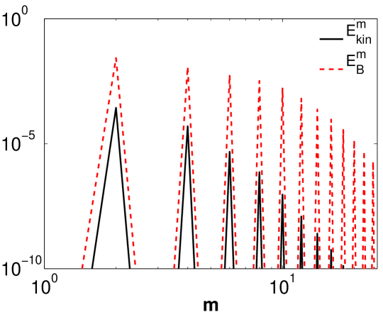
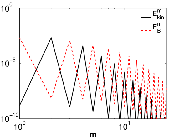
Figure 4: (Color online) Power spectrum of the kinetic energy (black continuous line) and the magnetic energy (red dashed line) for $\mathrm{\overline{Re}}=130$ (top) and $\mathrm{\overline{Re}}=160$ (bottom)

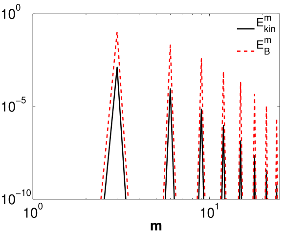
Figure 5: (Color online) Power spetrum of the kinetic energy (black solid line) and the magnetic energy (red dashed line) for $\mathrm{\overline{Re}}=130$ in a simulation in which modes with $m=3$ dominate.

In Figure 4 power spectra of the kinetic and magnetic energy of the simulations at $\mathrm{\overline{Re}}=130$ and $\mathrm{\overline{Re}}=160$ are shown. In the first case only even wavenumbers of the magnetic energy are amplified, whereas odd wavenumbers decreases in time. The opposite is seen in the second case, where odd wavenumbers of the magnetic energy are amplified and even wavenumbers decrease. The different symmetry of the magnetic field seems to be responsible for the decrease of the dynamo threshold, since this decrease correlates with the appearence of the odd wavenumbers in the magnetic field. In addition, Figure 5 shows the spectra of the simulations with $m=3$ as the dominant wavenumber, which have for $\mathrm{\overline{Re}_{h}}<\mathrm{\overline{Re}}<\mathrm{\overline{Re}_{s}}$ the same symmetry and accordingly the dynamo threshold is monotonously increasing.

For $\mathrm{\overline{Re}}>\mathrm{\overline{Re_{s}}}$, the critical $\mathrm{\overline{Rm}}$ first increases but then reaches a plateau at $\mathrm{\overline{Rm}}=600$. $Pm$ is less than 3 throughout the plateau region. It will now be argued that even more turbulent flows will not alter the critical $\mathrm{\overline{Rm}}$ significantly.

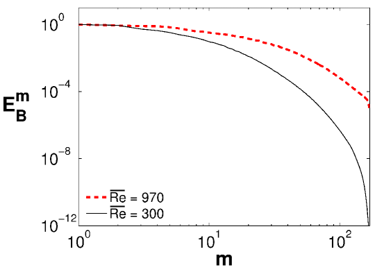
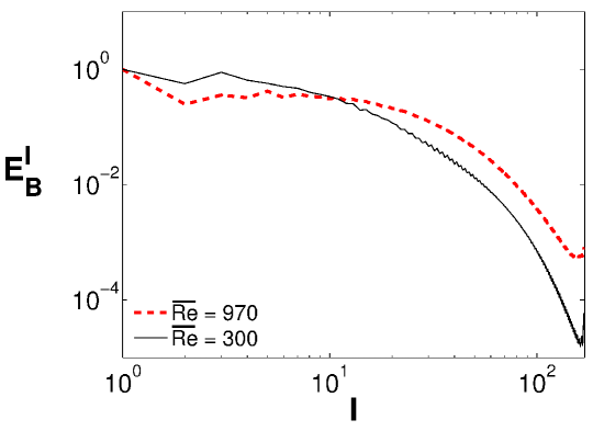
Figure 6: (Color online) Power spectrum of magnetic energy of spherical harmonic degree $m$ (top) and order $l$ (bottom) for $\mathrm{\overline{Re}}=300$ (black continuous line) and $970$ (red dashed line).

In the plateau region, the Reynolds number is high enough for the kinetic energy spectrum to decay as a power law as a function of both $m$ and $l$ with an exponent of -5/3. The phenomenolgy developed for small scale dynamos in Kolmogorov turbulence Schekochihin et al. (2004); Iskakov et al. (2007) therefore applies. According to this phenomenology, $\mathrm{\overline{Rm}}$ can increase as a function of $\mathrm{\overline{Re}}$ if $\mathrm{Pm}$ is larger than 1 and the eddies near the viscous length scale generate the magnetic field. If either $\mathrm{Pm}$ is small or the field generation occurs whithin the inertial range or at the integral scale, $\mathrm{\overline{Rm}}$ is independent of $\mathrm{\overline{Re}}$. In spherical Couette flow, the large scales are already capable of dynamo action. Not surprisingly, the spectra of magnetic energy peak at small $m$ and $l$ (see Fig. 6). Only the computation at the largest $\mathrm{\overline{Re}}$ raises doubts because the spectrum of magnetic energy reaches a second local maximum at $l=11$ in this case, which nevertheless is still within the inertial range (see Fig. 1) and at any rate below the global maximum at $l=1$. $\mathrm{Pm}$ is already slightly below 1 in this computation so that a further increase in $\mathrm{\overline{Re}}$ should only add a high wavenumber tail to the kinetic energy spectrum corresponding to eddies with too small a magnetic Reynolds number to contribute to the dynamo effect. In order to further test whether the small scales are responsible for magnetic field generation, eqs. (2,3) were solved simultaneously, but the axisymmetric components of the velocity were removed before the induction term in eq. (2) was computed. The magnetic field decayed in this simulation, which shows that the turbulent eddies in this velocity field are unable to support the magnetic field by themselves.

Since the magnetic field is generated at large scales even for $\mathrm{Pm}\approx 1$, an increase in $\mathrm{\overline{Re}}$ and concomittant decrease in $\mathrm{Pm}$ adds scales which contribute neither to the creation nor the destruction of the magnetic field. It is concluded that $\mathrm{\overline{Rm}}=600$ is the critical value of $\mathrm{\overline{Rm}}$ in more turbulent flows as well. In an experiment with $\mathrm{Pm}=10^{-5}$ this corresponds to $\mathrm{\overline{Re}}=6\times 10^{7}$. For Reynolds numbers this large, $E_{\text{kin}}$ is nearly independent of the Reynolds number according to fig. 2 and equal to 0.023, from which one deduces $\overline{v_{\text{rms}}}=0.058$ and $\mathrm{Re}\approx 10^{9}$. For the sodium experiment in Maryland with a gapwidth of $d=1m$ and a viscosity $\nu\approx 10^{-6}m^{2}/s$, this corresponds to a rotation period of about only $6ms$.

To conclude this section, we compare the stability diagram in fig. 3 with the results of similar studies. All numerical simulations report a general increase of the critical $\mathrm{Rm}$ with the Reynolds number for $\mathrm{Pm}$ larger than 1, an effect which is also found in the analytical model of ref. Boldyrev and Cattaneo (2004). The dependence of the dynamo threshold on the Reynolds number is not monotonous, however, and other published results have in common with fig. 3 a maximum in the critical $\mathrm{Rm}$ for $\mathrm{Pm}$ around 1. This feature is seen in refs. Ponty et al. (2005); Iskakov et al. (2007). Explanations for this effect have been attempted in refs. Brandenburg and Nordlund (2011); Malyshkin and Boldyrev (2010) who attributed it to either the bottleneck effect in turbulent spectra or the helicity at the viscous scale in the velocity field.

Despite the similarities, it is doubtful whether there is a universal mechanism for the dependence of the dynamo threshold. For example, the plateau in $\mathrm{Rm}$ is reached for values of $\mathrm{Pm}$ ranging from 0.1 to 1 across the different studies, so that there are variations by an order of magnitude in the $\mathrm{Pm}$ at which the critical $\mathrm{Rm}$ is maximum. There is also no indication of a bottleneck in the spectra presented here which shows that the bottleneck is not necessary for the observed variation of the dynamo threshold. It remains an open question why there is a maximum in the critical magnetic Reynolds number as shown in fig. 3 in the spherical Couette system.

IV Rough surface

IV.1 Hydrodynamic characteristics

The critical $\mathrm{Re}$ found in the previous section is challenging to realize in experiments. The problem arises from the fact that the inner sphere needs to rotate faster in order to increase $\mathrm{\overline{Re}}$. But a faster rotation rate also thins the boundary layer at the inner sphere and reduces the volume of fluid directly coupled to the boundary motion. An obvious remedy is to mount blades on the inner surface. The boundary layer cannot be smaller than the surface roughness which ensures a better coupling of the fluid to the inner sphere at high rotation rates. In the following, the blades are modelled by a volume force as described in section II.

Due to the increased momentum transport, turbulence develops at lower rotation rates. The first nonaxisymmetric instability arises at $\mathrm{Re_{h}}=425$ $(\mathrm{\overline{Re_{h}}}=95)$ with a dominant wavenumber of $m=2$, and beyond $\mathrm{Re_{s}}=465$ $(\mathrm{\overline{Re_{s}}}=108)$ odd wavenumbers increase, too. The evolution of the boundary layer thickness is shown in Figure 7 (top). As expected, the thickness of the boundary layer does not drop below one tenth of the gap width and approaches the thickness of the forced layer at large $\mathrm{Re}$. Since the thickness of the layer in which momentum is injected into the fluid remains nearly constant, independend from the rotation rate, the kinetic energy increases with $\mathrm{\overline{Re}}$. It does so approximately in $\mathrm{\overline{Re}}^{1/2}$, which is shown in Figure 7 (middle).

The torque on the inner sphere is zero for free slip boundary conditions so that one deduces from the energy budget (10) that the dissipation rate is given by $\epsilon=\int\bm{F}\cdot\bm{v}dV$. As can be seen in the bottom panel of fig. 7, $\epsilon$ behaves differently depending on whether the boundary layer is thicker than the forced layer or not. The interval of Reynolds number in each regime is too small to deduce a law relating $\epsilon$ with $\mathrm{Re}^{\prime}$.

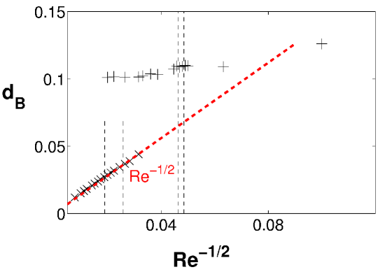
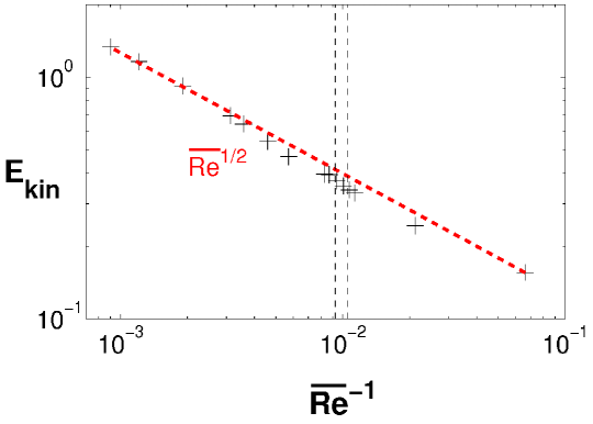
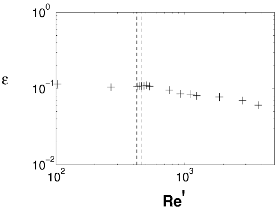
Figure 7: (Color online) Boundary layer thickness $d_{B}$ plotted against $\mathrm{Re}^{-1/2}$ (top), kinetic energy plotted against $\mathrm{\overline{Re}}^{-1}$ (middle), and energy dissipation rate plotted against $\mathrm{Re}^{\prime}$ (bottom). The vertical dashed lines show transitions to different regimes. Results obtained for smooth and rough surfaces are indicated by the symbols $\times$ and +, respectively.

IV.2 Dynamo transition

The diagram of the dynamo threshold plotted in the $(\mathrm{\overline{Re}},\mathrm{\overline{Rm}})-$plane in Figure 8 is similar to Figure 3. There is no dynamo action for axisymmetric flows. Similar to the simulations with no-slip conditions, even wavenumbers ($m=2$ and harmonics) increase in the magnetic energy spectra, whereas the total magnetic energy is increasing exponentially with superposed oscillations. In contrast to the simulations of the previous section, it was not possible to find a case in which the odd wavenumbers dominate the magnetic spectrum. Like in the simulations with no-slip conditions the dynamo threshold shows a plateau at $\mathrm{\overline{Rm}}=600$. In experiments with $\mathrm{Pm}=10^{-5}$ this corresponds to $\mathrm{\overline{Re}}=6\times 10^{7}$. By extrapolating the kinetic energy in Figure 7 (bottom) up to this $\mathrm{\overline{Re}}$, one gets $E_{\text{kin}}\approx 300$ and $\overline{v_{\text{rms}}}\approx 6.6$, or $\mathrm{Re}^{\prime}\approx 9\times 10^{7}$ with $\Omega^{\prime}_{i}=9.4$.

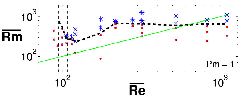
Figure 8: (Color online) Dynamo transition (black dashed line) with the same symbols as in figure 3.

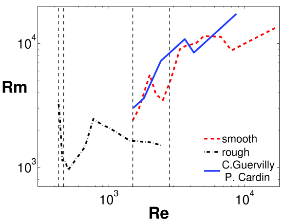
Figure 9: (Color online) Dynamo threshold of both surface types and results of Guervilly and Cardin (2010).

V Conclusion

Laminar spherical Couette flow with a stationary outer sphere is axisymmetric and consists of a differential rotation superimposed on a meridional circulation, which flows from the inner to the outer sphere in the equatorial plane, continues towards the poles of the outer sphere along the outer boundary in each hemisphere, and finally returns to the inner sphere. Dudley and James Dudley and James (1989) showed that flows of this type are capable of dynamo action. At the magnetic Reynolds numbers accessible by numerical computation, laminar spherical Couette flow nonetheless is not a dynamo due to the unfavourable velocity profile. For instance, the outward flow is concentrated in a narrow jet in the equatorial plane. Unstable spherical Couette flow on the other hand readily generates magnetic field. However, the field generation process still occurs at large scales, the small turbulent scales on their own do not support the magnetic field in these dynamos.

The numerical data allow us to extrapolate to more turbulent flows than the simulated flows if the data are plotted in terms of Reynolds numbers, magnetic and hydrodynamic, based on the rms velocity rather than the boundary velocity. The data are more difficult to interpret and extrapolate if they are given as functions of the Reynolds numbers computed with the inner boundary velocity as seen in Figure 9. This plot also includes the data from ref. Guervilly and Cardin (2010), which should be compared to our simulations with smooth boundaries. The curves are broadly similar apart from a shift by roughly a factor 1.5 along the $\mathrm{Re}-$axis, which must be attributed to the different aspectio ratio and the different magnetic boundary conditions.

If the flow is driven by the volume force which simulates blades of height one tenth of the gap size mounted on the inner sphere, the dynamo threshold expressed as critical magnetic Reynolds number based on the rms velocity is reduced by one sixth. Such a change is plausible because the topology of the flow is the same as for smooth boundaries, but the kinetic energy is more evenly distributed in space. Both the boundary layer and the equatorial jet are thicker. From an experimental point of view, the much more important improvement brought about by the blades is the reduction of the rotation rate of the inner sphere at the dynamo onset. The critical Reynolds number based on the rotation frequency of the inner sphere is reduced by a factor 10 by the blades. Using the results obtained with the simulated blades and the numbers for the Maryland experiment with a gapwidth of one meter and the viscosity of liquid sodium $\nu\approx 10^{-6}m^{2}/s$, a Reynolds number number of $\mathrm{Re}^{\prime}=9\times 10^{7}$ is reached for a rotation period of the inner sphere of 0.07 $s$. A spherical Couette dynamo is more readily attainable with blades mounted on the inner sphere because they improve the coupling between the fluid and the motion of the inner sphere and at the same time modify little the structure of the flow.

References

- Gailitis et al. (2000) A. Gailitis, O. Lielausis, S. Dement’ev, E. Platacis, A. Cifersons, G. Gerbeth, T. Gundrum, F. St efani, M. Christen, H. Hänel, et al., Phys. Rev. Lett. 84, 4365 (2000).
- Muller and Stieglitz (2002) U. Muller and R. Stieglitz, Nonlinear Processes in Geophysics 9, 165 (2002).
- Monchaux et al. (2007) R. Monchaux, M. Berhanu, M. Bourgoin, M. Moulin, P. Odier, J. F. Pinton, R. Volk, S. Fauve, N. Mordant, F. Petrelis, et al., Phys. Rev. Lett. 98, 044502 (2007).
- Lathrop and Forest (2011) D. P. Lathrop and C. B. Forest, Physics Today 64, 40 (2011).
- Dudley and James (1989) M. Dudley and R. James, Proc. R. Soc. Lond. A. 425, 407 (1989).
- Guervilly and Cardin (2010) C. Guervilly and P. Cardin, Geophys. Astrophys. Fluid Dynamics 104, 221 (2010).
- Schekochihin et al. (2004) A. Schekochihin, S. Cowley, J. Maron, and J. McWilliams, Phys. Rev. Lett. 92, 054502 (2004).
- Iskakov et al. (2007) A. B. Iskakov, A. A. Schekochihin, S. C. Cowley, J. C. McWilliams, and M. R. E. Proctor, Phys. Rev. Lett. 98, 208501 (2007).
- Ponty et al. (2005) Y. Ponty, P. D. Mininni, D. C. Montgomery, P. J.-F., H. Politano, and A. Pouquet, Phys. Rev. Lett. 94, 164502 (2005).
- Triana (2011) S. A. Triana, Ph.D. thesis, Faculty of the Graduate School of the University of Maryland (2011).
- Tilgner (1999) A. Tilgner, Int. J. Numer. Mech. Fluids 30, 713 (1999).
- Dumas and Leonard (1994) G. Dumas and A. Leonard, J. Comp. Phys. 111, 205 (1994).
- Hollerbach et al. (2006) R. Hollerbach, M. Junk, and C. Egbers, Fluid Dynamics Research 38, 257 (2006).
- Tilgner (2008) A. Tilgner, Phys. Rev. Lett. 100, 128501 (2008).
- Reuter et al. (2009) K. Reuter, F. Jenko, A. Tilgner, and C. B. Forest, Phys. Rev. E 80, 056304 (2009).
- Boldyrev and Cattaneo (2004) S. Boldyrev and F. Cattaneo, Phys. Rev. Lett. 92, 144501 (2004).
- Brandenburg and Nordlund (2011) A. Brandenburg and A. Nordlund, Reports on Progress in Physics 74, 046901 (2011).
- Malyshkin and Boldyrev (2010) L. M. Malyshkin and S. Boldyrev, Phys. Rev. Lett. 105, 215002 (2010).