Estimating the frequency of extremely energetic solar events, based on solar, stellar, lunar, and terrestrial records

Abstract

The most powerful explosions on the Sun – in the form of bright flares, intense storms of solar energetic particles (SEPs), and fast coronal mass ejections (CMEs) – drive the most severe space-weather storms. Proxy records of flare energies based on SEPs in principle may offer the longest time base to study infrequent large events. We conclude that one suggested proxy, nitrate concentrations in polar ice cores, does not map reliably to SEP events. Concentrations of select radionuclides measured in natural archives may prove useful in extending the time interval of direct observations up to ten millennia, but as their calibration to solar flare fluences depends on multiple poorly known properties and processes, these proxies cannot presently be used to help determine the flare energy frequency distribution. Being thus limited to the use of direct flare observations, we evaluate the probabilities of large-energy solar explosions by combining solar flare observations with an ensemble of stellar flare observations. We conclude that solar flare energies form a relatively smooth distribution from small events to large flares, while flares on magnetically-active, young Sun-like stars have energies and frequencies markedly in excess of strong solar flares, even after an empirical scaling with the mean activity level of these stars. In order to empirically quantify the frequency of uncommonly large solar flares extensive surveys of stars of near-solar age need to be obtained, such as is feasible with the Kepler satellite. Because the likelihood of flares larger than approximately X30 remains empirically unconstrained, we present indirect arguments, based on records of sunspots and on statistical arguments, that solar flares in the past four centuries have likely not substantially exceeded the level of the largest flares observed in the space era, and that there is at most about a 10% chance of a flare larger than about X30 in the next 30 years.

SCHRIJVER ET AL. Frequency of extreme solar events C.J. Schrijver Lockheed Martin Advanced Technology Center, 3251 Hanover Street, Palo Alto CA94304, USA (schrijver@lmsal.com) J. Beer, EAWAG, Swiss Federal Institute of Aquatic Science and Technology, Postfach 611 CH-8600 Duebendorf, SWITZERLAND (beer@eawag.ch) U. Baltensperger, Paul Scherrer Institute, Laboratory of Atmospheric Chemistry, CH-5232 Villigen PSI, SWITZERLAND (urs.baltensperger@psi.ch) E.W. Cliver, Space Vehicles Directorate, Air Force Research Laboratory, Sunspot, NM 88349, USA (ecliver@nso.edu) H.S. Hudson, Space Sciences Laboratory, University of California, Berkeley, CA 94720, USA (hhudson@ssl.berkeley.edu) M. Güdel, University of Vienna, Department of Astronomy, Türkenschanzstr. 17, A-1180 Vienna, AUSTRIA (manuel.guedel@univie.ac.at) K.G. McCracken, Institute for Physical Science and Technology, University of Maryland, MD, USA (jellore@hinet.net.au) R.A. Osten, Space Telescope Science Institute, 3700 San Martin Drive, Baltimore, MD 21218, USA (osten@stsci.edu) Th. Peter, ETH Zürich, Institut für Atmosphäre und Klima, CHN O 12.1, Universitätstrasse 16, 8092 Zürich, SWITZERLAND (thomas.peter@env.ethz.ch) D.R. Soderblom, Space Telescope Science Institute, 3700 San Martin Drive, Baltimore, MD 21218, USA (drs@stsci.edu) I.G. Usoskin, Sodankylä Geophysical Observatory (Oulu unit), P.O. Box 3000, FIN-90014, University of Oulu, FINLAND (ilya.usoskin@oulu.fi) E.W. Wolff, British Antarctic Survey, High Cross Madingley Road, Cambridge, CB3 0ET, UNITED KINGDOM (ewwo@bas.ac.uk)

1 Introduction

The Sun displays explosive and eruptive phenomena that span a range of at least a factor of $10^{8}$ in energy, from the present-day detection limits for “nanoflares” and the eruptions of small fibrils up to large, highly-energetic “X-class” flares and coronal mass ejections. At the lowest energies, millions of such events occur each day above the detection limit of $\sim 10^{24}$ ergs. The largest observed solar flares, with energies substantially exceeding $10^{33}$ ergs, occur as infrequently as once per decade or less.

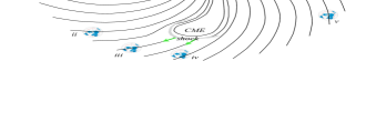
Figure 1: Illustration of visibility and propagation of solar explosive and eruptive events (modified after Reames, 1999; for an MHD simulation see, e.g., Rouillard et al., 2011), viewed from different orbital phases of Earth (i - v; not to scale) clarifying that flares (seen as photons) and energetic particle events are related, but that their detection depends on the evolution of the event on the Sun, on the heliospheric counterpart of any eruption (CME), and on the perspective from Earth (or a distant satellite, like the STEREO spacecraft). An eruption at position $A$ may be confined to the solar magnetic field, never reaching the heliosphere; depending on the magnetic geometry, solar energetic particles (SEP; green arrows) may escape into the heliosphere, following the Parker spiral of the field and detectable (as a rapid SEP event) near Earth only for orbital phases around i. An eruption at position $B$ could lead to a near-instantaneous SEP event for orbital phases around iii and later shock-accelerated (gradual) SEPs at phases iii-iv. Streaming-limit saturation of the SEP flux density would be observed for orbital phases iii - iv, with the SEP flux density exceeding the streaming limit when the shock front crosses Earth for phase iv.

Solar events have an increasing potential to impact mankind’s technological infrastructure with increasing flare energy, most effectively in the range of X-class flares, i.e. from a few times $10^{31}$ ergs upward [[, see, e.g.,]]severeswx2008,fema2010,kappenman2010,swximpactlloyds2011,jason2011.

Solar flares are the observed brightenings that result from a rapid conversion of energy contained in the electrical currents and in the magnetic field within the solar corona into photons through a chain of processes that involves magnetic reconnection, particle acceleration, plasma heating, and ionization, eventually leading to electromagnetic radiation. Large solar flares (defined here as involving energies in excess of some $10^{31}$ ergs) can accelerate particles to high energies and are generally associated with coronal mass ejections in which matter and magnetic field are ejected into the heliosphere at velocities of up to $\approx 3,000$ km/s. The ejections often drive shocks in which more accelerated particles are generated within the low corona and in the heliosphere. Due to these processes, solar flares are frequently associated with solar energetic particle (SEP) events near Earth (see, e.g., the reviews by [Benz (2008), Schrijver (2009)]). We discuss the relationships between these and other aspects of solar and space weather in some more detail in Sec. 2.

Large solar events drive episodes of severe space weather, including strong geomagnetic storms, enhanced particle radiation, pronounced ionospheric perturbations, and powerful geomagnetically-induced Earth currents, all of which affect our technological infrastructure from communications to electric power (Space Studies Board, 2008). It is therefore of substantial interest to establish the probability distribution for the largest solar flares and their associated energetic particle events and coronal mass ejections.

Direct measurements of the energies involved in solar events have been within the realm of the possible only since the beginning of the space age. Whereas the instrumental record spans almost eight decades, it begins with H$\alpha$ monitoring, with observation of flare ionizing radiation and energetic particles (initially by indirect means) as well as radio emission added over time, eventually culminating in global solar coverage only since 2011 with a patchwork of passbands that range from $\gamma$-rays to radio that can, with difficulty, be linked into a comprehensive view of the energies involved (e.g., Emslie et al., 2004, 2005). Hence, the frequencies of solar coronal storms that may occur only once per century, or even less frequently, remain to be established.

As we have only a limited understanding of the formation of magnetically-active solar regions and of their explosive potential, we have no theoretical framework that can be used to extrapolate the observed energy distribution of solar flares to energies that lie beyond the observed range. Sun-like stars provide evidence that larger magnetic explosions are possible, with observed energies that exceed the largest observed solar flares by at least three orders of magnitude. But, as we discuss in later sections, such stars are typically much younger and thus magnetically much more active than the present-day Sun, and with generally different patterns in their dynamos as reflected, for example, in the existence of high-latitude or polar activity and in the general lack of simple cycle signatures (e.g., Berdyugina, 2005; Hall, 2008). Can the Sun still power events substantially larger than, say, a large, infrequent X30 flare, and, if it can, how likely are such events? How likely are solar energetic particle events of various magnitudes?

In this study, we evaluate and integrate the available evidence to quantify the frequency distribution of the most energetic solar events. To this end, we combine direct observations of photons emitted by solar flares with those of their stellar counterparts. Such a comparison offers the advantage that observing an ensemble of Sun-like stars enables us to collect statistics on the equivalent of thousands of years of solar time, albeit subject to the problem that stellar flares are typically observed on stars that are much more active than the Sun has been at any time in recent millennia.

The association of solar flaring and frequent attendant CMEs with energetic particle events offers complementary sources of information on the statistics of extreme solar coronal storms. First, energetic particles leave observable signatures when they cause nuclear reactions in rocks that are exposed to them, such as lunar rocks (Nishiizumi et al., 2009), and even in terrestrial rocks that are protected by the Earth’s magnetosphere and atmosphere. Second, such energetic particles induce nuclear reactions in the terrestrial atmosphere which leave radioactive fingerprints in a variety of forms, including cosmogenic radionuclides ¹⁴C and ¹⁰Be, that can be traced in the geosphere as deposited, e.g., in polar ice or in trees. Third, the particles impacting the Earth’s upper atmospheric layers are expected to cause shifts in the chemical balance which may leave identifiable signatures in precipitation records; in particular, this pathway to long-term records on extreme solar events has been suggested for nitrate concentrations in polar ice (Sect. 4).

Each of these indirect measures (which we discuss in Sects. 3 and 4) offers its own difficulties related to its specific geochemical properties and the transport from the atmosphere into its archive. For example, ¹⁴C forms CO₂ and enters the global carbon cycle where it becomes heavily smoothed in time; ¹⁰Be spikes are subject to fluctuations of the climate and weather, both on Earth and throughout the heliosphere; exposed rock faces can only tell us about the cumulative effect of solar energetic particles over the lesser of the decay time of the radionuclides involved and the duration over which a rock face is exposed to solar particles. All of these radionuclide records sit on top of a background that is associated with galactic cosmic rays, which themselves are modulated on time scales upward of a few years by the variable solar wind, the heliospheric magnetic field, and the terrestrial magnetic field. Chemical signatures, as we discuss below, offer even greater difficulties, and we conclude that we do not currently see a way to use nitrate concentrations as indicators of SEP events.

In addition to these challenges in understanding the temporal modulations and integration of the records of solar energetic particles, there are challenges related to the creation and propagation of these particles before they are recorded. The relative importance of flares and CME-driven shocks for large SEP events continues to be debated: SEPs are generated both during the initial phases of a flare and in the propagation of CME shocks into and through the heliosphere. Line-of-sight photons and magnetically guided SEPs follow distinct pathways to Earth, so that flares and SEP events at Earth may be poorly correlated in time, contributing to a complex statistical relationship between the phenomena. Establishing their relationship requires that we understand the angular widths of the particle distributions entering into, and generated within, the heliosphere compared to the $2\pi$ solid angle available to flare photons. Another complication, yet to be properly understood, involves the propagation of the SEPs through the heliosphere, which appears subject to a saturation effect referred to as the “streaming limit” (Sect. 6). Some of the geometrical considerations involved in the flare-SEP correlation in observations at Earth are illustrated in Fig. 1. These and other issues are discussed in subsequent sections in the context of the available literature.

Transport of energetic particles in the geomagnetic field and atmosphere, including a nuclear atmospheric cascade/shower, is relatively well understood (e.g., Vainio et al., 2009). Whereas the transport of galactic cosmic rays (i.e., energetic particles originating outside the heliosphere) through the heliosphere is relatively well understood (e.g., Jokipii and Kóta, 2000; Potgieter et al., 2001; Caballero-Lopez and Moraal, 2004), the propagation of solar energetic particles – sometimes called solar cosmic rays – (i.e., those originating from a flare site or from a heliospheric shock associated with a solar eruption) is subject to substantial uncertainties (see Section 6). The parameters that set the spectral shape of the particle energy distribution are mostly empirically determined, adding additional difficulties when seeking to quantify the most energetic events that have been rarely observed, in particular for possible very rare events that have never been observed directly at all.

In Section 2 we present a brief overview of the connection between solar flares and energetic particles before they enter the detection systems in the form of spacecraft, ground-based detectors, rocks, ice, or biosphere. This section is mainly meant for readers who are relatively unfamiliar with these processes and their terminologies. After this brief introduction of some of the issues to be dealt with when using photons and tracers of energetic particles to learn about solar energetic events, we proceed to integrate solar, stellar, lunar, and terrestrial records in our attempt to establish the probability distribution of the largest solar energetic events.

Sections 3 and 4 lead to the finding that SEP records cannot be used to put tight constraints on the statistics of the largest solar flares, at least at present. The use of cosmogenic radionuclides to constrain SEPs near Earth is discussed in Section 3. In Section 4 we review the evidence, obtained in conjuction with this study, that nitrate concentrations in ice deposits cannot, at present, be used to learn about SEP events because the analyses of multiple ice cores has recently cast doubt on the suggestion that spikes in nitrate concentrations correlate with SEP events; ice nitrate concentrations may yet be validated as a quantitative metric for SEP events, but at present, the correspondence needs to be viewed at most as possible. Sections 3 and 4 clarify why, in the end, we have to rely on direct observations of flares. These two sections discuss constraints on the flare energy frequency distribution that turn out to be weak at best; they could be skipped on first reading.

Solar and stellar observations do provide interesting information on the flare energy distribution over many orders of magnitude: the comparison of solar and stellar flare observations in various segments of the electromagnetic spectrum is discussed in Section 5.

Section 6 contains an evaluation of the transformation of direct SEP and flare observations to a common scale for the source strengths near the Sun.

Flares and eruptions take their energy from the magnetic field within active regions; the implications of active-region sizes compared to the energies involved in flares and CMEs are described in Section 7.

We integrate the various findings in a discussion in Section 8.

2 Flares, CMEs, photons and energetic particles

“Flares” are, by definition, relatively rapid brightenings in the photon spectrum of the Sun and other stars. The signatures of flares can be found from very high-energy $\gamma$-ray emission to km-wave radio emissions. The bulk of a flare’s energy is radiated at visible wavelengths (see Section 5), but because of the bright background of the photospheric emission, flares have the highest contrast at X-ray, EUV, and radio emissions. Consequently, solar flare monitors generally report on the X-ray signature of the solar spectral irradiance.

Flares on stars other than the Sun, involving, for example, fully convective late-M type dwarf stars or somewhat evolved stars of near solar mass in tidally locked binary systems, share many of the characterizing properties of solar flares. Stellar flares reported on in the literature (e.g., Audard et al., 2000; Güdel, 2004; Stelzer et al., 2007; Walkowicz et al., 2011) are generally much more energetic than even large solar flares, but that is mostly because of the observational constraints of having to measure these stellar flares against the full-disk background coronal emission in stars that are X-ray bright, i.e., typically young, rapidly-spinning stars compared to the rather slowly rotating Sun (e.g., Güdel et al., 2003).

The thermal emission of flaring ranges from below a million degrees for the smallest events observed in quiet-Sun ephemeral regions to at least 100 MK for large-energy stellar events (e.g., Osten et al. (2007); see Sect. 5.2 for a discussion of some of the largest stellar flares observed to date). In emissions characteristic of high energies (providing direct or indirect measurements of non-thermal particle populations or direct measurements of high-temperature thermal emission), solar and stellar flares alike show fast rise and exponential decay phases (sometimes summarily characterized as “FRED”). As flares transition from the impulsive (fast-rise) to the decay phase, the spectral irradiance typically follows the so-called Neupert effect (Neupert, 1968; Veronig et al., 2002b): lower-energy emissions (e.g., soft X-rays) behave, to first order, as the time integral of high-energy emissions such as hard X-rays, non-thermal radio emission, or near-UV (or U-band) emission (for some examples of the Neupert effect in stellar flares, see Güdel et al. (2002) for the dM5.5 star Proxima Centauri; Güdel et al. (1996) for the M5.5Ve star UV Ceti; Hawley et al. (2003) for the dMe star AD Leo; and Osten et al. (2004) for the K1IV+G5IV binary HR 1099).

Solar flares are typically characterized by the NOAA/GOES magnitude scale which measures the peak brightness (increasing in orders of magnitude as A, B, C, M, and X, each followed by a number from 0 to 9.9 measuring the peak brightness within a decade). Many flares (often ’compact flares’) are characterized by impulsive brightenings and rapid decays, bringing most of the solar spectral irradiance back to near-preflare levels within a matter of minutes to tens of minutes; other “long-duration flares” can have a gradual rise and decay, sometimes lasting more than a dozen hours. Not only are the time scales different, the peak emissions occur from hard X-rays to relatively long-wavelength EUV, shifting overall to lower energies during the decay phase of any given flare, while differing between compact and eruptive flares, and between active-region flares and quiet-Sun filament eruptions that lead to CMEs (e.g., Benz, 2008). Consequently, the GOES classification scheme is not unambiguously useful as a metric for total flare energies; we discuss this problem in Section 5.

Whereas the distinct appearance of flares of different magnitudes and phases of evolution in different passbands complicates the bolometric calibration sought in this study, it is likely to play a role in enabling us to detect stellar flares against the full-disk background. The fact that flares shift through X/(E)UV wavelengths as a function of their magnitude and evolutionary phase restricts the range of flare energies that shows up in any such passband; this limits the “depth” of the distribution function, i.e., the ratio of largest to smallest flare observable within a given passband (e.g. Güdel et al., 2003), leaving the largest flares to stand out against the relatively weakened composite background. Even then, the “background” itself contains, and may be dominated by, a composite of flares, cf. the discussion by Audard et al. (2003) of a long observation of the M-dwarf star binary UV Ceti which shows continuous variability with no well-defined non-flaring level.

The broad wavelength range involved in solar and stellar flares makes it hard to observe the bolometric behavior of flares directly, because observations are typically limited to a relatively narrow bandpass. Hence, transforming the measured signal to an estimated bolometric fluence involves rather uncertain transformations, as discussed in Section 5.

Whereas flare photons from Sun and stars are detectable with present-day instrumentation, they leave no signatures that enable us to look back in time. SEPs that impact Earth or other solar-system bodies do leave such signatures, but their generation and transport introduce a range of challenges to be dealt with before SEP signatures can be used to quantify the frequency spectrum of solar flare energies.

Over 40 years ago, Lin (1970) presented evidence that there are two principal ways in which particles are accelerated at the Sun: (1) a process associated with reconnection in solar flares that has type III (fast-drift) radio bursts as its defining meter-wave radio emission and electrons with energy of $\sim 10$ keV as its characteristic particle acceleration ; and (2) acceleration at a shock wave manifested by a (slow-drift) type II metric burst, which is thought to reflect acceleration of escaping electrons and protons at all energies. Kahler et al. (1978) suggested that the type II shocks associated with SEP events were driven by CMEs, a suggestion that has found increasing support (Gopalswamy et al., 2002; Cliver et al., 2004; Gopalswamy et al., 2005).

By the mid-1980s the basic two-class picture of SEP acceleration was strengthened by elemental-composition and charge-state measurements of ³He and higher-mass ions. The observations revealed that the ³He and Fe abundances in the flare (type III) SEP events were enhanced by about a factor of $10^{3}-10^{4}$ and 10, respectively, relative to that in the shock (type II) events, and that Fe charge states were characteristically higher in the flare events (around 20 in flares versus $\sim 11-14$ for the large SEP events associated with shocks), see the review by Reames (1999).

The original “two-class” paradigm was challenged in the late 1990s when several large (and therefore presumably shock-associated) SEP events exhibited the elemental composition and charge states of the flare/reconnection SEP events (see Cliver, 2009, for a historical review of SEP research). Over time, these unusual large events were interpreted (e.g., Tylka et al., 2005; Tylka and Lee, 2006) in terms of particle acceleration in quasi-perpendicular shocks of “remnant” seed particles remaining in the low corona and inner heliosphere from earlier flares. Around the maximum of the solar cycle, when flares are most frequent, enhanced ³He SEP populations are observed in situ near Earth some $60$% of the time (Wiedenbeck et al., 2003). It is presumed that these remnant populations are also present near the Sun where they can be acted on by shocks. Because the remnant particles have the composition and charge state characteristics of flare-accelerated particles, the resulting SEP event looks like a high-energy flare-event, even though the ultimate accelerator is a shock.

Ground-based neutron monitors and ionization chambers have observed some 70 so-called ground-level enhancements (GLEs) in the past seven decades, indicating the presence of fluxes of ions in the energy range $1<E<20$ GeV, which will have produced radionuclides. If the initiating solar activity was within about $45^{\circ}$ from central meridian, however, the interplanetary CME will more strongly scatter GCRs, resulting in temporary decrease in the GCR intensity at Earth (Lange and Forbush, 1942), commonly referred to as a “Forbush decrease”. The cosmogenic radionuclide formation at Earth may, in some cases, be overcompensated by the Forbush decrease with an associated reduction in GCRs by about 10% for about a week (Usoskin et al., 2008), but the details of that depend on the conditions of the event (Reames, 2004). For example, solar eruptions near the western limb produce the most intense GLEs, and contain the highest fluxes of particles with energies in excess of 5 GeV, while in this case there typically is no Forbush decrease at Earth.

We note that for SEP proxies with a long mixing time scale within the Earth’s atmosphere prior to deposition (specifically for the ¹⁰Be concentration discussed below) there is the additional complicating factor that SEP-induced increases in the proxy ride on top of variations associated with the GCR variations that are associated with variations in the heliospheric magnetic field and the solar wind on time scales of years or more. To differentiate between, say, large-fluence SEP events and extended cycle minima, one has to make assumptions about the heliosphere that are difficult to validate.

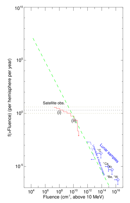
Figure 2: Downward-cumulative frequency distribution (red) of fluences of solar energetic particle (SEP) events of fluences $F$ or larger (for particles with energies in excess of 10 MeV) for satellite observations (histogram), and for upper limits derived from lunar radionuclides (blue) and terrestrial records (${}^{14}C$ upper limit shown by a (blue) dashed line). The green dashed line shows the slope of the fit to the flare energy frequency distribution from panel a for comparison, scaled to go through the kink in the satellite-based SEP fluence frequency distribution. Labels (i) and (ii) are discussed in the last paragraph of Sect. 6.

Within the heliosphere, SEP propagation may be subject to a “streaming limit” for particles escaping from a shock acceleration region. This is a type of saturation effect caused when protons streaming from the shock are hampered by their propagation in their own enhancement of the upstream waves (Reames and Ng, 2010), whose existence is an essential component of the theory of diffusive shock acceleration. This streaming limit does not apply near the shock, so SEP fluxes can exceed the streaming limit when a shock passes directly over Earth, or over a satellite outside the geomagnetic field.

3 Radionuclides as tracers of past solar energetic particle events

3.1 Extraterrestrial radionuclides

A direct way to determine the statistics of solar energetic particle events is to measure energetic particles with space-based instrumentation. A compilation of the fluences for such events for particle energies exceeding 10 MeV is shown as a red histogram in Fig. 2 (based on data from McCracken et al. (2001)). These data are naturally limited to event frequencies exceeding once per fifty years, as that is the current span of the observational record. On the low-fluence side the range of accessible energies in the frequency spectrum is limited by the detection threshold against the GCR background.

Some information on events that are much rarer than once per century can be extracted from ’exposures’ that have lasted much longer than a few decades. SEPs that impact solar-system bodies leave traces in the form of a mixture of radioactive nuclides. The production of cosmogenic radionuclides from the exposure to SEPs can be calculated for a specified elemental composition of the rock and a given shape of the differential energy spectrum using Monte Carlo simulations (Reedy and Masarik, 1994). In a rock, only the time-integrated production rate (a balance between production and decay) is recoverable. The integration time depends on the half-life of the radionuclide in question. As a consequence of the much steeper energy spectrum of SEPs compared to that of GCRs, SEPs only produce cosmogenic radionuclides in the outermost layers of the rocks. This differentiation between GCRs and SEPs as a function of depth creates a natural spectrometer that enables correction for the contribution from GCR-induced production, although this does require assumptions on the SEP energy spectrum in order to thereby estimate upper limits of the frequency of SEP events (see Usoskin (2008), and references therein).

When rocky material from the Moon is analyzed, we have access to the cumulative dose of SEPs without the complicating factors of terrestrial magnetic and atmospheric shielding or the effects of a dynamic weathering environment. The combined results of lunar rock studies, compiled by Usoskin (2008), assuming that the upper limits to the fluences are associated with a few events over the isotopes’ life time, are shown in Fig. 2. These upper limits emphasize the downturn seen at the high-fluence end of the frequency distribution of satellite SEP observations, but they are not particularly restrictive in establishing the shape of the spectrum or the strength or fluence of a possible largest SEP event size.

3.2 Cosmogenic radionuclides on Earth

The combination of the SEP fluence frequencies measured by satellites and the upper limits based on the analysis of lunar rocks shown in Fig. 2 illustrates the need to fill a gap for events with cumulative frequencies of less than once per few decades. In this section, we discuss one possibility that is currently being explored, which is the measurement of terrestrial radionuclides stored in a stratified manner that enables setting tighter limits on lower-fluence events.

Terrestrial cosmogenic radionuclides are produced mainly by spallation-type nuclear interactions between high-energy (GeV) particles and nuclei of the dominant atmospheric constituents (N, O, Ar). After production, those radionuclides that end up stored in naturally stratified “archives” such as ice deposits, trees, and sediments, prove most useful to our purpose.

Records of cosmogenic radionuclides provide blended information about the solar magnetic activity, the strength of the geomagnetic dipole field, and atmospheric transport and deposition processes. By using independent information about the geomagnetic dipole field, and by combining different records of ¹⁰Be from ice cores with ¹⁴C from tree rings, a rather clean signal of the variations in the GCRs due to varying levels of solar activity can be extracted for at least the past 10,000 years. That record reveals the variability of the solar dynamo and the associated heliospheric magnetic field on time scales ranging from decades to millennia, with grand minima and maxima throughout the long record (Solanki et al., 2004; Vonmoos et al., 2006; Usoskin et al., 2007; Steinhilber et al., 2008, 2010; McCracken et al., 2011).

Not only the long-term variations can thus be recovered: there is some promise of recovering shorter-term spikes, albeit that these are washed out by the transport process between generation and deposition, while set against a variable background of the solar dynamo. The time it takes to transport a newly produced cosmogenic radionuclide from the atmosphere into an archive depends mainly on the altitude at which it is produced. This ranges from weeks for the troposphere to years for the stratosphere (Raisbeck et al., 1981; Field et al., 2006). As a consequence, the production signal stored in the archive is smoothed and the temporal resolution is limited to about one year at best. The higher the desired temporal resolution, the more the signal will be influenced by transport processes. Over the past 5 years, the use of global circulation models (GCM) has greatly improved our understanding of the manner in which atmospheric transport processes influence the deposition of ¹⁰Be and other radionuclides into polar ice (Field et al., 2006; Heikkilä et al., 2009).

To produce cosmogenic radionuclides a primary (galactic or solar) cosmic ray needs energies above about 500 MeV with a specific yield function depending on the particular isotope. Because of the relatively low energies in SEPs (compared to GCRs) the majority of them can only enter the Earth’s atmosphere at high magnetic latitudes (exceeding about $60^{\circ}$). Moreover, again because of the relative softness of the SEP energy spectrum, the contribution to the cosmogenic isotope production of most of the SEP events that can be observed by satellites in orbit is too small to be detected in ice, rocks, or biosphere against the background production of a radionuclide from GCRs. Some large SEP events, however, include solar cosmic rays with energies in excess of 10 GeV; these are efficient producers of cosmogenic radionuclides. Their relative contribution to an annual GCR production is small (Usoskin et al., 2006). This is particularly true for ¹⁴C and ¹⁰Be (³⁶Cl is more sensitive to lower energies and is therefore a promising candidate to study strong SEP’s, but as ³⁶Cl is produced by spallation of the relatively rare ⁴⁰Ar this reduces the temporal resolution for standard-sized ice cores or requires considerably larger ice samples to measure it with the required signal-to-noise contrast).

SEP’s recorded by particle detectors during the past 50 years show a range of fluences and spectral steepness. Very large SEP events from activity near solar central meridian typically have higher fluences, yet steeper spectra, which makes them deficient in particles exceeding 1 GeV. Very large SEP events from near the west limb of the Sun typically have lower fluences but flatter spectra, favoring particle energies in excess of 1 GeV (Van Hollebeke et al., 1975).

All of the above effects needs to be factored in when translating radionuclide concentrations to SEP fluences. This leads to substantial differences in estimates. For example, there are three ¹⁴C production models that differ markedly in their estimates of SEP fluences. The first estimate was made by Lingenfelter and Ramaty (1970), based on an empirical parametrization of early measurements of neutron fluxes in the Earth’s atmosphere. It predicts that the average SEP production rate for a year is $\sim 6$% of the GCR annual rate, and that the event of 1956/02/23 (the largest observed ground level enhancement – GLE – by neutron monitors (e.g., Rishbeth et al., 2009), with a very hard spectrum) would give 1/3rd of the overall annual ¹⁴C production. It is important to note that Lingenfelter and Ramaty (1970) made the rather extreme assumption that the magnetic shielding is reduced by a factor of 5 during large solar storms, which leads to a high ¹⁴C production rate.

The next estimate was based on a semi-empirical model by D. Lal (Castagnoli and Lal, 1980; Lal, 1988), who adjusted numerical calculations to fit empirical data. That model yields an average production for ¹⁴C by SEP events being less than 1% on average, while the event of 1956/02/23 would yield only several percent of the annual radiocarbon production (Usoskin et al., 2006).

A more recent model based on an extensive Monte-Carlo simulation of the atmospheric particle cascade (Masarik and Beer, 1999, 2009) suggests that SEPs contribute, in an average year, only 0.03% to production of ¹⁴C. This very small value may be caused by the neglect of the atmospheric cascade (and thus neutron capture channel of ¹⁴C) in their model (cf. Masarik and Reedy, 1995). The most recent Monte-Carlo model (Kovaltsov et al., 2012) suggest that the average contribution of SEPs into the global ¹⁴C is about 0.2%.

Thus, the model predictions differ by more than two orders of magnitude. For the purpose of the present study, we opt for the most conservative upper limit currently published, based on the work by Masarik and Beer (1999, 2009): to achieve this, we took the data by Lingenfelter and Hudson (1980), and shifted them upward in fluence by two orders of magnitude. These data, shown in Fig. 2, support a substantial drop below any power law that can be fit to the satellite observations for events with cumulative frequencies larger than once per century. The ¹⁴C data are clearly more restrictive in that respect than the lunar rock data, in that they lie further below the trend found in the directly observable fluence range.

Calculations by Usoskin et al. (2006) and Webber et al. (2007), based on the measured spectra of the largest SEP in the past 50 years, predicted undetectable effects for ¹⁰Be, ¹⁴C and ³⁷Cl assuming global atmospheric mixing, or a barely detectable effect if ¹⁰Be is dominated by polar production. This is a consequence of (a) the large amplitude of the GCR modulation by the sunspot cycle that dominates the contributions by SEPs, and (b) the high standard deviation ($\sim$15%) of annual ¹⁰Be data. Larger SEP events may have happened in the past, however, and increased sample sizes, multiple cores extending back thousands of years, and better understanding of the heliospheric variability on GCR fluxes may make it possible to use radionuclides to inform us on the SEP fluence frequency distribution as shown in Fig. 2 for frequencies below once per few decades. But achieving such results requires considerable analysis, well beyond what is feasible in the present study.

4 Nitrate concentrations in ice, and the possible link to solar particle events

When solar energetic particles impact the Earth’s atmosphere they cause ionization in the polar regions that results in production of NO (Jackman et al., 1990, 1993, 2008). The NO is interconverted to other odd nitrogen species, and some of it, at whatever altitude it is produced, should ultimately end up deposited in snowfalls as nitrate (in aerosol or scavenged from gaseous HNO₃), if not destroyed prior to that by chemical interactions at mesospheric and higher layers. Given that SEPs most readily enter the Earth’s atmosphere at high geomagnetic latitudes, and because long-lived ice is readily found at high geographic latitudes, it is logical to seek a nitrate signal in polar ice cores.

Dreschhoff and Zeller (1990) reported on the analysis of two ice cores from Windless Bight in Antarctica in which they measured the nitrate concentration going back to about 1905 AD. The Antarctic record was later supplemented by a core from Summit in Greenland (GISP2 H core) which was measured at a sampling density of 10 to 20 samples per year (for samples of 1.5 cm in thickness) extending back to 1561 AD.

The Summit core contains spikes in the nitrate concentration that are superposed on a regular seasonal cycle. These spikes are often just 1 sample wide but occasionally 2-3 samples wide, i.e., occur in a period that could range from a single snowfall up to about 3 months. The core contains a continuous spectrum of spikes, from many small ones, to over one hundred large to very large ones: the largest spikes are about a factor 5 larger than the typical seasonal cycle amplitude. Dating of these spikes is achieved by counting annual layers in the cores, supplemented by identification of deposits associated with strong known volcanic eruptions. With that information, the year should be accurately known near the volcanic markers (32 over the 430-y record), but might deviate by a year or two away from such markers.

The coincidence of some of these spikes with known space-weather events suggested that at least the strongest among them might originate from SEP events. In particular, the strongest (integrated) peak in the Summit-core record was dated to within a few weeks of the 1859 Carrington event, one of the largest known solar flares and associated CME sequences to impact geospace (Dreschhoff and Zeller, 1994; Shea et al., 1993; McCracken et al., 2001; Tsurutani et al., 2003; Cliver and Svalgaard, 2004; Shea et al., 2006).

The timing and sharpness of the nitrate spikes is problematic if nitrate is indeed associated with SEPs, because it is difficult to transport nitrates from above the tropopause quickly enough into tropospheric snowfalls within a matter of at most a few weeks. Furthermore, one would not expect nitrate produced in the middle atmosphere to be deposited over such a short time period, nor would one expect troposheric enhancements by a large factor, as observed in the spikes. This could be resolved if the snow is actually recording a tropospheric, rather than a stratospheric, production of nitrate. Alternatively, if the SEP event is having its effect higher in the atmosphere, it may be accompanied by one of the rare (especially in Antarctica) sudden stratospheric warming events which could transport material downwards relatively rapidly, perhaps allowing a response within a month or two. However, the coincidence of two such rare events would be unusual. Otherwise, one would expect a transport time of order 6 months, and thus no sharp signal in the ice core chemical patterns.

Strong nitrate spikes may be caused by terrestrial events or by depositional processes. It has been well documented that nitrate spikes associated with enhanced ammonium concentrations are an indication of biomass burning, and these are seen in Greenland ice cores, including those from the Summit regions where the H core was taken (e.g., Legrand et al., 1992; Whitlow et al., 1994; Fuhrer and Legrand, 1997). Spikes can be induced by changes in scavenging efficiency owing to, for instance, changes in the degree of riming (the inclusion of supercooled droplets as snow crystals grow). More specifically, spikes in nitrate deposition are induced by conversion of nitric acid to aerosol through association with either sea salt (for coastal Antarctica) or ammonia (for central Greenland) leading to deposition of the associated aerosol (Wolff et al., 2008).

In the work leading up to this manuscript, Wolff et al. (2012) assembled information on a total of 14 ice cores with high time resolution from both arctic and antarctic regions, at various geomagnetic latitudes. They found that apart from the Summit GISP2 H ice core, no nitrate signatures were found in the ice dated to 1859. Several nitrate spikes of a similar nature were found in all the Greenland cores, including one from the Summit site. However, all such spikes including one dated to 1863 (the nearest large spike to 1859 in the later records), were associated with an ammonium spike. In the cores where other components were measured, black carbon and vanillic acid (diagnostic of combustion plumes in general, and wood burning, respectively) were found in each large spike between 1840 and 1880. None of these components were measured in the H core, so Wolff et al. (2012) cannot conclusively identify the origin of the peak labelled as 1859, but do conclude that it is inevitable that most nitrate spikes in all Greenland cores are of biomass burning origin. While it may be possible to isolate very large events that are not of such origin, Wolff et al. (2012) conclude that even the 1859 event was not large enough to give a signal in most ice cores. It is unfortunately apparent that the statistics of nitrate cannot provide the statistics of SEP events so that this potential proxy for SEP events prior to the mid 20th Century can, at present, neither be used to estimate the frequency spectrum of SEP events nor to set unambiguous upper limits to a possible historical maximum for such events. In view of this, the nitrate data shown in figures by McCracken et al. (2001) and Usoskin (2008) are not included in Fig 2.

5 Flare energies

5.1 Solar flares

In order to compare the occurrence frequencies of solar and stellar flares as a function of their energy, the diversity of available measurements needs to be transformed to a single unified scale. Here, we attempt to rescale the observations to bolometric fluences, based on available approximate conversions.

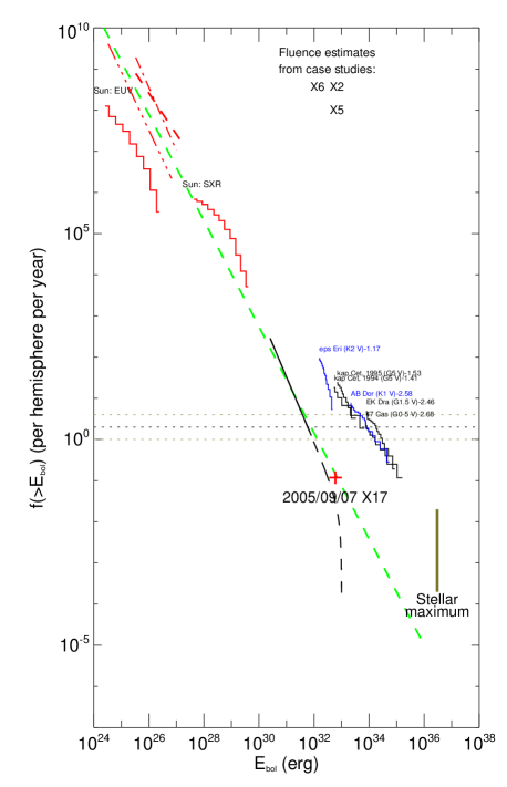
Figure 3: Downward-cumulative frequency distribution for bolometric flare fluences, $E_{\rm bol}$. Quiet-Sun EUV microflares: solid histogram: Aschwanden et al. (2000); dash-dotted: Krucker and Benz (1998); dashed-triple-dotted: Parnell and Jupp (2000); dashed: Benz and Krucker (2002). Lower red histogram: active-region soft X-ray flare data from Shimizu (1995, 1997). The dashed black curve shows Eq. (2) for $F_{\rm max}=10^{33}$ ergs; the empirical range of a power-law approximation is shown solid. A red cross marks the fluence of the 2005/09/07 X17 flare at an equivalent cumulative frequency for it to be the 5th largest flare since 1976 (see http://www.spaceweather.com/solarflares/topflares.html). Histograms for $E_{\rm bol}\mathrel{\mathchoice{\vbox{\offinterlineskip\halign{\hfil$\displaystyle#$\hfil\cr>\cr\sim\cr}}}{\vbox{\offinterlineskip\halign{\hfil$\textstyle#$\hfil\cr>\cr\sim\cr}}}{\vbox{\offinterlineskip\halign{\hfil$\scriptstyle#$\hfil\cr>\cr\sim\cr}}}{\vbox{\offinterlineskip\halign{\hfil$\scriptscriptstyle#$\hfil\cr>\cr\sim\cr}}}}10^{32}$ ergs are for active Sun-like main-sequence stars (black or blue for spectral type G or K), scaled as in Eq. (5). The vertical bar marks the largest flare fluence in Sun-like stars in Kepler observations. The green dashed power law, with index $-2.3$, approximately connects the solar data. The central dotted line shows the frequency at which CME opening angles reach $2\pi$ radians (with its uncertainty range).

For solar flares, characteristically $\approx 70$% of a flare’s total radiative energy is emitted at visible wavelengths (characterized by a blackbody temperature of approximately $9000$ K; see, e.g., Woods et al. (2004); Fletcher et al. (2007); that value is also found for stellar flares, see, e.g., Hawley and Fisher (1992)). This can be used to begin the comparison of energy scales to the GOES flare classification scale, Fig. 3 shows (at the top) the total energy estimates for three well-studied solar flares (of classes X2, X5, and X6; Aschwanden and Alexander, 2001; Benz, 2008), assuming that these X-ray and EUV estimates are complemented by another 70% of the total energy to make the bolometric fluence as described above. These flares suggest that the average X4.3 flare would have a bolometric fluence of $4.9\times 10^{32}$ ergs.

Woods et al. (2006) provide excess total solar irradiance (TSI, i.e., the flare fluence) estimates for four very energetic flares. Two of those, which occur well away from the solar limb, are X17 and X10 flares with fluences of $6.0\times 10^{32}$ ergs and $2.6\times 10^{32}$ ergs, respectively. The average of these fluences is about that estimated above for an average X4.3 flare, beginning to illustrate the uncertainties in the conversion process to a common bolometric scale.

On average, only $\approx 0.6\pm 0.1$% of the total photon energy is emitted in the GOES $1-8$ Å channel that is used to classify flares by their peak intensity(Emslie et al., 2005; Kretzschmar, 2011). These numbers, derived from composite observations of C-class to X-class flares (Kretzschmar, 2011) require an average multiplier of $\approx 160\pm 30$ to convert a fluence derived from the GOES $1-8$ Å passband to a bolometric fluence. For comparison, direct total solar irradiance measurements for four large flares (Woods et al., 2006) suggest multipliers of $\approx 49-162$, with values of $126$ and $162$ for the two flares (X17 on 28 Oct. 2003 and X10 on 29 Oct. 2003) well away from the solar limb, roughly consistent with the abovementioned average conversion.

In his study, Kretzschmar (2011) differentiates flares into four groups (C4-M2.8, M2.8-M6.4, M6.4-X1.3, and X1.3-X17) and uses a superposed epoch analysis for all flares within these subgroups to derive conversion factors from GOES $1-8$Å fluences to SOHO/VIRGO bolometric (or total solar irradiance, TSI) fluences. The conversion factors for the four subgroups are $330\pm 130$, $220\pm 80$, $140\pm 60$, and $90\pm 10$. These results show a decrease in the conversion factor with increasing flare magnitude, for TSI fluences from $0.36\times 10^{31}$ ergs to $5.9\times 10^{31}$ ergs. The conversion factor for the group of X-class flares is some 35% lower than those described above, which may be a consequence of differences in samples or, for example, be influenced by positions on the solar disk. In the remainder of this study we use a power-law approximation of the conversion from $1-8$Å GOES fluence to TSI fluence provided by Kretzschmar (2011),

$$F_{\rm TSI}=2.4\times 10^{12}F_{\rm GOES}^{0.65\pm 0.05},$$ (1)

although we give preference to direct bolometric fluences for those large flares for which these where published.

Other estimates of bolometric flare energies are available in the literature, but generally these are subject to assumptions that may cause these estimates to be significantly different from direct observations of the total solar irradiance (TSI), so they are excluded here (for example, the energy in $>20$ keV electrons in the X28+ flare on 2003/11/04 has been estimated to be of order $\approx 1.3\times 10^{34}$ erg (Kane et al., 2005), but see Tranquille et al. (2009) for an alternative view of the implications of these observations).

GOES observations revealed a soft X-ray ($1-8$ Å) flare fluence distribution (Veronig et al., 2002a) that transforms to a downward-cumulative distribution function for bolometric fluences(applying Eq. 1)) of

$$N^{\ast}_{f}(F_{b})=9.2\times 10^{33}\,\left({1\over F_{b}^{1.03\pm 0.09}}-{1\over F_{\rm max}^{1.03\pm 0.09}}\right),$$ (2)

where $F_{\rm max}$ is a possible cutoff fluence beyond which no flares occur (discussed below). In deriving this distribution, Veronig et al. (2002a) did not correct for the background X-ray emission beneath the flare emission; such a correction would be important for relatively small flares, but as we focus on M-class flares and larger (with the above power law approximation valid only starting at mid-C class flares), the effects are limited and ignored below.

The largest observed flare saturated the GOES detector and was estimated to peak at X28, not much above the X10 and X17 flares discussed above. Hence, for the purpose of illustration (and arguments below) we assume a value of $F_{\rm max}=10^{32}$ ergs, about twice the abovementioned average flare fluence for the X10 and X17 flares as a lowest likely upper limit to flare fluences. This would approximately correspond to an X25 flare using the scaling that GOES soft X-ray fluence $F$ and the GOES flare class (the peak brightness) $B$ are related through

$$F\propto B^{1.10}$$ (3)

(Veronig et al., 2002a). Fig. 3 shows the above distribution for $F_{\rm max}=10^{33}$ ergs as a dashed black curve.

This distribution is based on 8400 flares from 1997 through 2000 for which GOES $1-8$Å fluences were specified; the power law holds for flares with a range of $1-8$ Å GOES fluences from $\approx 6\times 10^{27}$ to $\approx 10^{30}$ ergs. The normalization of the annual frequency distribution in Eq. (2) and Fig. 3 for an average over a full solar cycle is achieved by setting the frequency for an M1-class flare to the average frequency of 140 per year for flares of M1 or larger over the period of cycle 23, from 1996/01/01 to 2007/01/01, and taking a value of $4\times 10^{30}$ ergs as the bolometric fluence for a characteristic M1 flare from Kretzschmar (2011).

For flares below GOES class C, the determination of the flare frequency distribution from the disk-integrated GOES signal becomes increasingly ambiguous for less-energetic events. As one goes down the energy scale, the signal from individual flares sinks into the background soft X-ray luminosity. Moreover, the flare photon spectrum weakens in X rays and strengthens in the extreme ultraviolet (EUV) for flares of decreasing magnitude. For the study of less energetic events, spatially-resolved X-ray or EUV imaging is more appropriate. One such study used Yohkoh soft X-ray images (Shimizu, 1995, 1997) to estimate flare energies from imaging observations of an active region and its immediate surroundings in a field of view of 5 arcmin square. These are observations of only a single moderately large active region. The histogram in Fig. 3 shows the results of this study assuming that averaged over a solar cycle 3 such regions exist on the disk, and using the estimate that 70% of the energy is emitted at visible rather than X/EUV wavelengths.

For even smaller flares, several energy fluence distributions are available based on either the SOHO/EIT or TRACE EUV observations (Krucker and Benz, 1998; Parnell and Jupp, 2000; Aschwanden et al., 2000; Benz and Krucker, 2002). In order to convert these energies to estimated bolometric fluences we use the finding that approximately 15% of the event energy is emitted in the coronal EUV, as derived for larger flares (Kretzschmar, 2011), although this has not been verified for the smaller events observed in the EUV only. The differences between the four distributions shown are related to different algorithms for flare characterization and to assumptions about the geometrical extent of the observed events along the line of sight (Aschwanden et al., 2000) .

For the remainder of this study we are primarily interested in the largest flares, but we point out that it is intriguing that these solar flare distributions align relatively well, within the substantial uncertaintites in energy conversions and from the perspective of a log-log diagram. A rough power-law approximation (shown by the green dashed line in Fig. 3, is given by

$$N(E_{f}){\rm d}E_{f}\propto E_{f}^{\alpha_{f}}{\rm d}E_{f},$$ (4)

with $alpha_{f}=-2.3\pm 0.2$, with an estimated uncertainty that is largely associated with the uncertainties in the conversions from X-ray and EUV fluences to bolometric fluences for microflares to large solar flares.

5.2 Stellar flares

Solar flares are a manifestation of the Sun’s magnetic field, and that field is believed to arise from the interaction of convection with rotation, especially differential rotation: the dynamo mechanism. Other stars with convective envelopes (G, K, and M spectral types) also show magnetic activity, including flares. Here we will discuss G- and K-type stars because they are most similar to the Sun. Stellar flares cannot be resolved spatially and so we can detect only energetic events that produce sufficient contrast against the visible photosphere or the X-ray/radio corona. In addition, stellar observations often are available for only a limited wavelength range and so it is difficult to gain a full bolometric view of an event. Detectable high-energy flares have been seen on rapidly-rotating GKM stars because the rotation enhances the magnetic field. Single GKM main sequence stars lose angular momentum with age and so the flaring stars are either very young (up to $\sim 100$ Myr old), or they are in close binaries where tidal interaction causes spin-up of an older star; these latter systems are known as BY Dra binaries (main sequence) or RS CVn binaries (evolved). Stellar flares have been reported with X-ray or EUV energies as low as $\sim 10^{28}$ ergs (Güdel et al., 2002); this corresponds to a bolometric fluence $\sim 3-5$ times higher. Most reports on stellar flaring report fluences much larger than that simply because of the difficulty of detecting small flares against the bright background of the overall corona or photosphere.

More energetic flares have harder emission, and so the passband used biases the detection threshold. Observations in the shorter-wavelength X-rays tend to favor the largest flares, making the energy distribution appear less steep than it really is. This has been seen explicitly in BeppoSAX observations with soft (about 0.2-2 keV) and hard ($>1$ keV) channels. Simultaneous observations on the same flares made in both bands led to a slope $\alpha=2.4\pm 0.2$ for the soft channel and $\alpha=2.0-2.2$ for the hard channel (Güdel et al., 2003). For this reason, it is preferable to search for flares and coronal radiation in either soft X-rays or the EUV.

Figure 3 shows stellar flare data for five G and K main sequence stars (from Audard et al., 2000) in soft X-ray and EUV bands ($0.01-10$ keV, or $1.2-1200$ Å), scaled to approximate bolometric fluences by assuming the same ratio between bolometric and coronal fluences holds as for solar EUV observations (see Sect. 5.1), i.e., that about 30% of an event’s energy is emitted in the EUV (excluding M-type stars which show comparable behavior but are far from solar in their basic properties; data from Audard et al., 2000). Little is known in the literature about the ratio of coronal to bolometric brightness during flares. One example of a large flare on an ultracool M8 dwarf star (Stelzer et al., 2006) showed comparable energies in the visible and soft X-ray passbands in which the flaring star was observed, in acceptable agreement with our assumption for purpose of comparison of solar and stellar data in Fig. 2. In the absence of further information, we make the simplest assumption, namely, that solar and stellar flare energies are, to first order, similarly distributed over the electromagnetic spectrum.

The five G- and K-type stars for which Audard et al. (2000) determined the flare frequency distributions are highly active and rotate much more rapidly than the Sun. The most active among these stars exhibit flaring at energies of $10^{33}$ erg several times per day. The studies by Osten and Brown (1999) and by Audard et al. (2000) revealed that the frequency of flaring in these stars increases nearly proportionally to the background stellar X-ray luminosity which spans a range of a factor of $10^{4}$ in their sample (their Fig. 4). Audard et al. (2000), for example, find a power-law index of $0.95\pm 0.10$ for the scalings between cumulative flare frequencies and coronal X-ray luminosity. For the comparison shown in Fig. 3 we assumed a purely linear dependence, so that the observed cumulative distribution of flare energies, $N_{\rm obs}(>E|L_{\ast,X})$, for a star with X-ray luminosity $L_{\ast,X}$ transforms to the distribution $N^{\odot}(>E)$ scaled to the solar X-ray luminosity, $L_{\odot,X}$ through

$$N^{\odot}(>E)=\left({L_{\odot,X}\over L_{\ast,X}}\right)N_{\rm obs}(>E).$$ (5)

This scaling shifts the stellar distributions downward in the diagram towards the solar distribution, while essentially collapsing them onto each other. In this scaling, we used an estimated average coronal luminosity for the Sun of $L_{\odot,X}=4.3\times 10^{27}$ erg s^-1, which is an average over the solar cycle for the $0.1-2.4$ keV bandpass (Judge et al., 2003).

The comparison of the solar and scaled stellar frequency distributions for flare energies in Fig. 3 shows that the frequency distribution for large solar flares lies substantially below the scaled stellar data. From this we conclude that the data on active stars cannot be used to infer the probabilities of solar flares of high energies that may or may not occur at frequencies below once per few decades.

In the decade following the work by Audard et al. (2000), energetic flares have been seen in G stars in the white-light bandpass ($\sim$ 4000-9000Å) of the Kepler mission. About 0.5% of the brightest G stars exhibit flares with fluences of $\sim 10^{34}$ up to $\sim 10^{37}$ ergs (Basri et al., 2011; Walkowicz et al., 2011). These are energies in the optical bandpass and so are lower limits since some energy is emitted at other wavelengths. Flares exceeding $10^{37}$ ergs have not yet been seen.

The G stars that show flares in the Kepler data most often show multiple flares, with some flaring about every other day. Most Kepler data is sampled every 30 minutes and so only very energetic, long-lived flares are reliably detected. However, a subset of stars is observed every minute and a few flaring stars have been so observed. In those cases it is possible to fully resolve the rise of a flare (with a time scale of $\sim 10$ min) and its decays (on time scales of hours), with secondary events during the decay (Soderblom et al., 2012). The very large sample size of Kepler (some 150,000 stars) corresponds to an effective monitoring time for a single average G star of $\sim 400,000$ years, far beyond anything previously done.

Another very energetic flare was reported for II Peg (K2IV+dM) at $10^{37}$ ergs (Osten et al., 2007; Ercolano et al., 2008). Other reports of very large flares include Kürster and Schmitt (1996) who observed a flare from the binary CF Tuc with radiated energy in the ROSAT bandpass of $1.4\times 10^{37}$ erg, and Endl et al. (1997) who reported on a large flare from HU Vir which had a radiated energy of $7.7\times 30^{36}$ ergs in the same bandpass; both of these targets are active binaries. One extreme value is $10^{38}$ ergs reported by Schaefer et al. (2000), but it remains to be seen if the source of the flare was correctly identified.

From the above, it appears that it is highly unlikely that any flare would exceed $10^{37}$ ergs on a Sun-like star in any phase during its evolution once it has comfortably settled on the stellar main sequence. But that leaves a factor of $\sim 10^{4}$ between the largest observed solar flare and the largest possible for a Sun-like star. Are there other empirical constraints that help us narrow that gap?

6 Mapping SEP fluences to flare energies

Figure 2 shows that the slope for flare electromagnetic fluences (Fig. 3) is very different from the slope seen for SEP fluences: the power-law exponent ($\mu$) in the frequency distributions of power-law form

$$dN/dx=Ax^{-\mu}$$ (6)

is smaller for SEP fluences – $\mu\approx 1.1-1.3$ in Fig. 2 below a fluence of about $5\times 10^{9}$ cm^-2 – than it is for flare electromagnetic emissions ($\mu=\alpha_{f}\approx 2.3$, see Eq. [4]), while the SEP event fluence spectrum turns to a significantly steeper spectrum above $\sim 5\times 10^{9}$ cm^-2 (see also Van Hollebeke et al., 1975). Several effects may be at play here: 1) SEP spectral distributions may depend on event energy (which could include a dependence on the partitioning between flare radiative and CME bulk-kinetic energies), 2) background corrections, 3) effects of compound events involving two or more CME/shocks on SEP size distribution, and 4) particle propagation effects in the heliosphere.

Before considering the effects of any of the above potential processes, we should allow for a geometrical effect that must play a role: dilution of the fluence over an opening angle into the heliosphere, and - related to that - the possibility that the SEP event misses the Earth altogether: as SEPs propagate into the heliosphere over a solid angle less than $2\pi$ we certainly need to correct for the probabibility that SEP events may not hit Earth and thus not be recorded, while if that opening angle depends on the energy of the event, then the SEP fluence needs to be corrected for the change of opening angle with total event energy. We can make the following plausible quantitative argument:

Following the reasoning by Schrijver (2011), although in part in the opposite direction, we start from the observation that the frequency distribution of particle fluences can be approximated by a power law up to about $5\times 10^{9}$ cm^-2:

$$N_{\rm p}{\rm d}F_{\rm p}\propto F_{\rm p}^{-\delta}{\rm d}F_{\rm p}.$$ (7)

Let us assume that the particles are emitted from their source region at or near the Sun into a solid angle $\Omega$ that is a function of the total energy $E_{\rm f}$ of the event, here chosen to be approximated by:

$$\Omega\propto E_{\rm f}^{\gamma}.$$ (8)

The value of $\gamma$ can be estimated by comparing the flare energy distribution in Eq. (4) with a distribution of opening angles, $a$ (in degrees), for eruptions from small fibril eruptions to large CMEs (summarized by Schrijver, 2010)

$$N_{a}{\rm d}a=b\,a^{-\beta}{\rm da},$$ (9)

with $\beta=2.0\pm 0.3$ (with $b\approx 1.1$ for $\beta=2$).

For given $a$ (expressed in radians), the corresponding fractional solid angle is given by

$${\Omega\over 4\pi}={1\over 2}(1-\cos{a})\approx{1\over 4}a^{2},$$ (10)

where the righthand exression holds for sufficiently small $a$. Using that expression with Eqs. (8), and (9), we find

$$N_{a}{\rm d}a\propto a^{{2\over\gamma}(1-\alpha_{f})-1}{\rm d}a.$$ (11)

With Eq. (9) we find $\gamma=2(\alpha_{f}-1)/(\beta-1)\approx 1.9\pm 0.6$.

If the particle fluence at Earth, $F_{p}$, is a fixed fraction $f$ of $E_{\rm f}$, diluted by expanding over a solid angle $\Omega$, then with Eq. (8),

$$F_{p}\propto f{E_{\rm f}\over\Omega}\propto E_{\rm f}^{1-\gamma},$$ (12)

transforming Eq. (4) to read

$$N_{\rm p}{\rm d}F_{\rm p}\propto F_{\rm p}^{{1-\alpha_{f}\over 1-\gamma}}{\rm d}F_{\rm p}.$$ (13)

As in this model experiment SEPs are assumed to be emitted within a solid angle $\Omega$, only a fraction

$$p={\Omega\over 4\pi}\propto E_{\rm f}^{\gamma}$$ (14)

of the total number of events can be detected near Earth. Hence, to derive the SEP fluence distribution from the flare energy fluences, Eq. (13) has to be multiplied by $p$:

$$N_{p}{\rm d}F_{\rm p}\propto F_{\rm p}^{{1-\alpha_{f}+\gamma\over 1-\gamma}}{\rm d}F_{\rm p}\equiv F_{\rm p}^{-\epsilon}{\rm d}F_{\rm p}.$$ (15)

With the values of the exponents above, we find $\epsilon=(\alpha_{f}-1)(\beta-3)/(\beta-2\alpha_{f}+1)=-0.8\pm 0.2$, consistent with the observations provided that we limit the comparison to events for which the SEPs are spread over a solid angle small compared to $2\pi$ steradians.

An opening angle of 180^∘ is reached for an event frequency of approximately twice per year (Schrijver, 2010), with an uncertainty of at least a factor of two. That range, shown by dotted horizontal lines in the panels of Fig. 3 and 2, lies just above the frequency where the SEP event fluence frequency distribution bends downward, suggesting that geometrical considerations may be a dominant effect in changing the slope of flare to SEP fluences at least around the range labeled ’(i)’ in Fig. 2, but not for energies at or above the value labeled ’(ii)’. In other words, the segment of the observed SEP fluence distribution function labeled ’(i)’ in Fig. 2 likely needs to be steepened to accommodate the above geometrical effects, and this steepening appears to bring it in line with the slope found for flare bolometric fluences, i.e., with the green dashed line. Therefore, the break in the SEP fluence spectrum above the downward kink could reflect a limit on the spreading of the SEPs in angle. We note, however, that we have insufficient information on the angular width distribution of SEP events in general: observations put many of these opening angles for impulsive events on a gaussian-like distribution with $\sigma=15^{\circ}-20^{\circ}$ (Reames, 1999) whereas recent STEREO observations have shown events with opening angles up to $136^{\circ}$ (Wiedenbeck et al., 2011). Nevertheless, this argument offers a plausible origin to the kink in the frequency distribution in Fig. 2 so that we cannot assume that kink is indicative of a change in the behavior of solar flare fluences for the largest flares.

7 Conversion of magnetic energy to power flares

Having established that currently available flare statistics on Sun-like stars are not directly applicable to the present-day Sun owing to the difference in mean activity level, and that lunar and terrestrial records leave a substantial range of uncertainty on the largest solar events, we explore one further avenue. The energy released in large solar coronal storms is ultimately extracted from the electromagnetic field in the solar atmosphere. Because that energy is associated with the surface magnetic field, including its sunspots, some constraint may be derivable from sunspot sightings.

One element of this argument is the observation that mature active regions - within a bounding perimeter including spots, pores, knots, and faculae - are characterized by a remarkably similar flux density, $B_{0}=\langle B\rangle$ of about $100$ Mx/cm² to $150$ Mx/cm² (Schrijver and Harvey, 1994) regardless of region size. This allows us to perform an order of magnitude scaling between the energy available for flaring in the magnetic field above an active region and the flux that this region contains.

If we assume that a fraction of $f=0.01-0.5$ of the magnetic energy density in a volume with a characteristic mean field strength of $B_{0}$ can be converted into what eventually is radiated from the flare site (e.g. Metcalf et al., 2005; Schrijver et al., 2008), the typical dimension $d_{0}$ and magnetic flux $\Phi_{0}=B_{0}d_{0}^{2}$ in such a flaring region are given by

$$d_{0}=\left({4\pi E_{f}/f\over B_{0}^{2}}\right)^{1/3}\,\,;\,\,\Phi_{o}=B_{0}d_{0}^{2}={(4\pi E_{f}/f)^{2/3}\over B_{o}^{1/3}}.$$ (16)

For a very large flare with energy $E_{f}=10^{37}$ ergs, we find $d_{0}\approx(2-7)R_{\odot}$ and $\Phi_{0}\approx(10-80)\,10^{24}$ Mx, even using $B_{0}=300$ G; to illustrate the magnitude of the problem, we chose a value of $B_{0}$ for this estimate that is, in fact, $2-3$ times higher than characteristic of solar regions (Schrijver, 1987; Schrijver and Harvey, 1994). Even with an average magnetic flux density substantially above what the present-day Sun shows us, the flaring region simply would not fit on the Sun. For flares with $E_{f}=10^{35}$ ergs, $d_{0}\approx(0.4-1.6)R_{\odot}$ and $\Phi_{0}\approx(0.3-4)\,10^{24}$ Mx. Although very sizeable, and requiring a relatively large average surface field strength, these numbers are still compatible with the size of the Sun. Are they compatible with the largest observed regions on the Sun?

The flux distribution for historically observed active regions reported on by Zhang et al. (2010) exhibits a marked drop below the power law for fluxes exceeding $\Phi\sim 6\times 10^{23}$ Mx, and they find no regions above $\Phi_{\rm max}\sim 2\times 10^{24}$ Mx. Historically, the largest sunspot group recorded occurred in April of 1946, with a value of 6 milliHemispheres (Taylor, 1989); for an estimated field strength of 3 kG, that amounts to a flux in the spot group alone of $\Phi_{\rm spots}\sim 6\times 10^{23}$ Mx. The total flux in this spot group was likely larger, but perhaps within a factor of $2-3$ of that in the spots, and thus of the same order of magnitude as the upper limit to the distribution found by Zhang et al. (2010).

Starting from that largest flux of $3\Phi_{\rm spots}\sim 1.8\times 10^{24}$ Mx for $B_{0}=100$ G and $f=0.5$, an upper limit for flare energies of $E_{f}=f\Phi^{3/2}/(4\pi B_{0})\approx 10^{33}$ ergs results, comparable to the excess-TSI fluence reported for well-observed X17 and X10 flares well-away from the solar limb reported by Woods et al. (2006) (see Sect. 5.1).

In other words, a solar flare with energy of a few times $10^{32}$ ergs is compatible with what we know about the largest solar active regions. A flare with an energy of, say, $10^{34}$ ergs would seem to require a spot coverage some 20 times larger than the historically observed maximum, or 12% of a hemisphere (the largest spot coverage for the Sun as a whole reported by the Royal Greenwich Observatory since 1874 is 0.84%). No such records of monster spots on the Sun have been historically reported or pre-historically recorded, so they are likely not to have occurred over the past centuries or even millenia. In fact, our simple scaling arguments suggest that an upper limit of close to the largest flares observed during the past three decades is consistent with the reported observations on the largest sunspot groups over the past few centuries.

8 Discussion and conclusions

We attempted to combine direct observational records of SEP events associated with flares and CMEs with upper limits based on lunar rock samples, terrestrial biosphere samples, and ice-core radionuclide concentrations to establish a frequency distribution of approximate particle fluences (Fig. 2). The lunar and terrestrial samples do constrain SEP fluences for the largest events, but only as upper limits for fluences well beyond the historical records obtained during the space age. Hence, this information cannot at present be used to significantly contribute to our knowledge of the frequency spectrum of flare energy fluences beyond the historically observed range that extends up to about X30.

We have had to conclude that nitrate concentrations in polar ice deposits cannot, at present, be used to extend the direct observational records of SEP events to a longer time base without at least significantly more study.

Once the multiple factors influencing the ¹⁰Be data are better understood, it may be possible to set an upper limit that will further constrain the event frequencies for high fluence events. This will include establishing a calibration from ¹⁰Be concentrations to SEP event fluences. Should such a calibration become available in the future, effects of limitations on the transport of energetic particles through the heliosphere (the “streaming limit” discussed in Sect. 2) shall need to be better understood before the ¹⁰Be upper limit can be mapped to solar flare energy fluences.

We present an argument that the “kink”’ in the $>10$ MeV SEP fluence frequency spectrum around $5\times 10^{9}$ cm^-2 does not necessarily reflect a change in the flare-energy spectrum, but may in fact be a consequence of geometrical effects related to the finite opening angle of SEP cones. This effect causes a decrease in detection frequency for smaller opening angles simply because events with smaller extent are more likely to miss the Earth, combined with a dilution of the fluence over that opening angle that affects the particle flux density. This argument is supported by the fact that the frequency at which the kink occurs corresponds relatively well with the frequency for which observed opening angles of CMEs approach $2\pi$ steradians. We therefore suggest that this kink likely does not reflect a change in the shape of the solar flare fluence distribution, but rather that it reflects the geometry of SEP generation and propagation.

The combination of solar and stellar flare observations shows that the Sun and a sample of younger, more active stars are not brought into alignment for their flare-energy frequency spectra even if their frequencies are scaled with the average background coronal luminosity of the star (based on an empirical scaling derived for stars in a range of activities much higher than that of the Sun). We shall need to trace how strongly the assumptions made in the conversion from X-ray/EUV fluences to bolometric fluences based on the solar flares affect this misalignment. But regardless of the outcome of that, this misalignment of solar and stellar data means (i) that currently available data on flares on very active stars cannot help us in our quest to determine frequencies of extremely large solar flares, and (ii) that in order for stellar data to be helpful in that respect, observations of stars of solar type as well as of roughly solar activity level are required to establish the X-ray/EUV properties of large stellar flares as well as their bolometric fluences in order to be able to enter them into a frequency-fluence diagram as we made here for solar flares.

The solar flare observations can be roughly approximated by a power law frequency distributions as in Eq. (4). If we start from the assumption that flare fluences follow this power-law parent distribution function with index $\approx-2.3$, we can establish how likely it is that we have a 30-y run of observations in which no flares are seen with energy fluences exceeding $\approx 10^{33}$ ergs - at a GOES class of roughly around X30, subject to a calibration uncertainty of at least 50% (see Sect. 5.1) - if the power law would in fact persist up to a cutoff of the most energetic among stellar flares, i.e., around $10^{37}$ ergs. We find that this would occur once in 10 30-y samples, which, although relatively unlikely, is not statistically incompatible with the observations. This does not provide us with a significant upper bound to solar flare energies by itself, but does provide a probability of at most 10% for any flare exceeding the presently observed maximum in the next 30 years.

We argue that flares with a magnitude well above the observational maximum of about $10^{33}$ ergs are unlikely to occur, however, by the argument presented in Sect. 7. Such flares would require that much of the solar surface be covered by strong kilo-gauss fields, exhibiting large sunspots that have not been recorded in four centuries of direct scientific observations and in millenia of sunrises and sunsets viewable by anyone around the world. For example, a flare with an energy of around $10^{34}$ ergs should require a spot coverage of just over 10% of a solar hemisphere, which would be readily visible even to naked-eye observers if it occurred. Sunspot records suggest that no regions were observed in the past four centuries that could power flares larger than those observed in the most recent three decades.

We conclude that flare energies for the present-day Sun have either a true upper cutoff or at least a rapid drop in frequency by several orders of magnitude below the scaled stellar frequency spectrum for energy fluences above about X40. Based on the direct solar observations and the indirect arguments presented in this study, solar flares with energy fluences above about X40 are very unlikely for the modern Holocene-era Sun. Setting significantly stricter quantitative limits than this for the most energetic solar flares than we have summarized in Fig. 3 requires that we observe a sample of several dozen very large flares on stars of solar type and of near-solar age. That, in turn, requires the equivalent of at least several thousand years of stellar time in the combined observational sample, to be observed in X-ray, EUV, or optical emissions. Additional, but less direct, limits could be inferred from estimated starspot coverages from many thousands of Sun-like stars in, e.g., observations being made by the Kepler satellite.