WU B 12-01
The () gamma transition form factor and the gluon-gluon distribution amplitude
P. Kroll 111Email: kroll@physik.uni-wuppertal.de
Fachbereich Physik, Universität Wuppertal, D-42097 Wuppertal,
Germany
and
Institut für Theoretische Physik, Universität
Regensburg,
D-93040 Regensburg, Germany
K. Passek-Kumerički 222Email: passek@irb.hr
Theoretical Physics Division, Rudjer Bošković Institute,
Zagreb, Croatia
Abstract
The and transition form factors are analyzed to leading-twist accuracy and next-to-leading order (NLO) of perturbative QCD. Using an mixing scheme and all currently available experimental data the lowest Gegenbauer coefficients of the distribution amplitudes for the valence octet and singlet and the gluon-gluon Fock components are extracted. Predictions for the vertex function are presented. We also comment on the new BELLE results for the transition form factor.
1 Introduction
The recent measurements of the photon to pseudoscalar meson transition form factors at large photon virtualities, , by the BaBar collaboration [1, 2] caused much excitement and renewed the interest in the theoretical description of these observables. Most surprising is the seemingly sharp rise of the form factor with the photon virtuality, which is difficult to accommodate in fixed-order perturbative QCD. Power corrections to the usual leading-twist (collinear) approach [3] seem to be required. However, there is also a measurement of this form factor by the BELLE collaboration [4] which shed doubts on the BaBar data. At large the results of the two measurements differ, the BELLE results are close to the theoretical expectations from the leading-twist approach. Also the and form factor data behave as expected according to theoretical analysis [5, 6, 7] of the CLEO [8] and L3 data [9], measured at lower than the BaBar data. Strong power corrections are not demanded in these analysis. Indeed a next-to-leading order (NLO) leading-twist analysis [6] is in reasonable agreement with the CLEO and L3 data. It is therefore tempting to reanalyze the and form factors to this accuracy along the lines presented in [6], taking into account the new BaBar data. It should be mentioned that the combined CLEO, L3 and BaBar data on these two form factors have already been analyzed in other approaches. Thus, for instance, in [10] factorization is exploited, and in [11, 12] in addition the non-valence quark contributions have been analyzed. In [13] light-front holographic QCD was used, in [14] the low data have been studied within the non-local chiral quark model and in [15] the dispersive representation of the axial anomaly is used to derive an expression for the form factors that holds at all . In [16] the anomaly sum rule has been used for the analysis of the transition form factors. A combined analysis of the low and high data has also been performed in [17].
In this work we analyze the and transition form factor data within the rigorously proven collinear factorization approach. We restrict ourselves to the region of fairly large , and assume that in this region of higher-twist and other power corrections are negligible. Thus, we have to deal with only a small number of free parameters
The and mesons possess singlet and octet quark-antiquark Fock components and, additionally, two-gluon ones leaving aside higher Fock states. Leading-twist distribution amplitudes, , are associated with each of these Fock components. This feature leads, on the one hand, to the well-known flavor mixing and, on the other hand, as a further complication, to mixing of the singlet and the gluon-gluon () distribution amplitudes under evolution. In the case of the transition form factors the two-gluon Fock components do not contribute to leading order (LO), they require higher orders of perturbative QCD (see Fig. 1 for relevant Feynman graphs). In our previous analysis [6] of the and transition form factors to NLO leading-twist accuracy the short lever arm provided by the range of the CLEO and L3 data, the overall number of the data as well as the size of their errors, made it impossible to fix precisely even the lowest Gegenbauer coefficients of the distribution amplitudes. Here, in this work we attempt a reanalysis of the form factors, using in addition to the CLEO and L3 data also the recent BaBar data [2]. With our analysis we want to demonstrate that the and form factor data can easily be accommodated by a QCD calculation to NLO leading-twist accuracy. And, on the strength of a larger set of data covering a substantially larger range of , a second goal of our analysis is better determination of the distribution amplitudes and the discussion of accompanying theoretical uncertainties. This is of utmost importance since the two-gluon Fock components play a role in many hard exclusive processes involving and/or mesons which are nowadays accessible to experiment. Thus, for instance, the vertex contributes to decay processes such as (see e.g. [18, 19]), to the hadronic production and to meson pair production in the central region of proton-proton collisions [20]. The two-gluon Fock components may also matter in decays in pairs of or mesons and they may be attributed to the enhancement of some of the channels in charmless decays as compared to the corresponding pion channels (e.g. [21, 22, 23]). An example is set by the channels for which such an enhancement is experimentally observed [24, 25]. In this context the form factors are of importance which are also affected by the component of the and mesons (e.g. [26]).
The plan of the paper is the following: In Sect. 2 we recapitulate properties of the and distribution amplitudes for the and mesons, in particular their evolution behavior. In Sect. 3 the mixing is briefly discussed. The CLEO [8] and BaBar [2] data on the transition form factors are analyzed for several scenarios in Sect. 4 and values for the second Gegenbauer coefficients of the three distribution amplitudes are extracted and discussed. We also shortly comment on the data for the time-like transition form factors obtained by BaBar [27] and implications of the resulting distribution amplitudes for the vertex. A brief comment on the transition from factor is given in Sect. 5. As usual the paper ends with a summary.


2 Properties of the distribution amplitudes
In this work we follow the definitions and convention used in [6]. For the convenience of the reader we summarize here the main ingredients necessary for understanding and used for obtaining the results of this work.
When considering the evolution and mixing of quark and gluon states under evolution, it is convenient to choose as valence Fock components of the pseudoscalar mesons the octet and singlet combinations of quark-antiquark states and the two-gluon state, , which also possess flavor-singlet quantum numbers and contributes to leading-twist order. Higher Fock components are neglected in our analysis since their contributions are power suppressed. It is to be stressed that the above states are partonic Fock components and not effective meson states or glueballs which are frequently considered in the treatment of - mixing.
In collinear approximation and to leading-twist accuracy a distribution amplitude, (, ), is associated with each of the Fock components we consider 333 A formal definition of the leading-twist distribution amplitudes in terms of particle-vacuum matrix elements of quark field operators or the gluon field strength tensor can be found in [6].. These quark distribution amplitudes are symmetric in and normalized to unity at any factorization scale , while the gluon distribution amplitude is antisymmetric and, consequently, there is no natural way to normalize it. The mixing of gluon distribution amplitude with the quark distribution amplitude under evolution removes this ambiguity and, as shown in [6], the change in gluon normalization is reflected in the change of off-diagonal anomalous dimensions governing the evolution. In [6] an attempt was made to give a detailed account of different conventions found in defining the gluon distribution amplitude throughout the literature
The distribution amplitudes can be expanded upon the Gegenbauer polynomials
| (1) |
where only the terms for even occur as a consequence of the symmetry relations. In terms of the expansion coefficients the mixing of the quark singlet and gluon distribution amplitudes are expressed by
| (2) |
where is the initial scale of the evolution and . The number of colors is denoted by and is the number of active flavors at the characteristic scale of the process. The coefficients of the eigenfunctions of the matrix evolution equation which introduces mixing between quark and gluon distribution amplitudes, are here denoted by . The powers are the eigenvalues of the matrix of anomalous dimensions [28, 29]
| (3) |
where the LO elements read in our convention
| (4) |
with . Note that we introduce the distinction between the quantity () which counts the (fixed valence) quark content of the meson’s flavor-singlet combination and the above defined , the number of active flavors at some scale, which appears in the functions and, as such, is connected to the running of the coupling constant. The parameters in (2) are given by
| (5) |
The evolution of the octet distribution amplitude is merely governed by and takes the simple form
| (6) |
As is well-known and can be seen from (1 - 6), the quark distribution amplitudes evolve into the asymptotic form
| (7) |
and the gluon one to zero for .
To the order we are working, NLO evolution of the quark distribution amplitude should in principle be included. To this accuracy the Gegenbauer polynomials are no longer eigenfunctions of the evolution kernel, i.e. their coefficients do not evolve independently [30]. The impact of the NLO evolution on the transition form factors is expected to be small compared with the NLO corrections to the subprocess amplitudes [31]. Therefore we refrain from considering NLO evolution here.
The full quark and gluon distribution amplitudes defined through hadronic matrix elements read and , respectively. The decay constants, , are, as usual, defined by vacuum-meson matrix elements of flavor singlet or octet weak axial-vector currents
| (8) |
The singlet decay constants, , depend on the scale but the anomalous dimension controlling it is of order [34]. In fact the evolution of is part of the NLO evolution of the singlet distribution amplitude, it represents the scale dependence of its first Gegenbauer coefficient. This is to be contrasted to the octet distribution amplitude for which the first Gegenbauer coefficient, , is 1 at all scales. Thus, in harmony with the neglect of NLO evolution of the distribution amplitudes, the scale dependence of is neglected too.
3 mixing
This section is devoted to the phenomenological aspects of mixing. The mixing scheme we are employing in this work is explained, numerical values listed, and results from the literature discussed.
As in [6], in order to reduce the number of independent distribution amplitudes we follow [39] and assume meson independence of the distribution amplitudes, i.e.
| (9) |
Hence, the mixing behavior of the valence Fock components and the particle dependence solely resides in the decay constants. Since in hard processes only small spatial quark-antiquark separations are probed, this assumption is sufficiently plausible - the decay constants play the role of wave functions at the origin of configuration space. We work in octet-singlet basis and for the decay constants we use the general parameterization [34, 39]
| (10) |
In [39, 40] it has been observed that mixing is particularly simple in the quark-flavor basis with valence Fock components and . In this basis which is supposed to separate strange and non-strange contributions, the mixing behavior of the decay constants is controlled by the angles and , defined analogously to (10). It turned out from phenomenology that these angles practically fall together , i.e. that we can write
| (11) |
This observation is supported by a QCD sum rule study [41]. A recent lattice QCD study [42] is also not in conflict with it. The occurrence of only one mixing angle in this basis is a consequence of the smallness of OZI rule violations which amount to only a few percent and can safely be neglected in most cases. symmetry, on the other hand, is broken at the level of .
But, although the, so-called, quark-flavor mixing scheme, which employs quark-flavor basis and one mixing angle, offers successful phenomenological description of mixing, the inclusion of states favors the octet-singlet basis. This is due to the fact that state mixes under evolution with just singlet state, in contrast to more complicated mixing with both and states when using quark-flavor basis. Thus when one considers two gluon states and evolution octet-singlet basis is natural and we use it in this work. Since for phenomenological insight the quark-flavor scheme is useful and a lot of results are obtained using this scheme, we present the useful transformation formulas for the valence Fock components of the basis states and
| (12) |
and
| (13) |
The new decay constants are related to and by
| (14) |
We see that in (12) the () Fock component appears in the () states, i.e., even if we start with pure and states the evolution produces the opposite states due to different evolution of SUF(3) octet and singlet states.
We now turn to numerical values of mixing parameters found in the literature. Working in the quark-flavor basis and exploiting the divergences of the axial-vector currents - which embody the axial-vector anomaly - the mixing parameters in the quark-flavor mixing scheme can be expressed in terms of the masses of the physical mesons [43], e.g.
| (15) |
Evaluation of the mixing angle provides . Using for the decay constant in the quark-flavor basis the symmetry result , one finds for the strange decay constant in that basis
| (16) |
Transforming these results to the octet-singlet basis, one obtains the results for the mixing parameters (10) that are quoted in Tab. 1. In [39, 40] the mixing parameters have been determined phenomenologically allowing for higher-orders flavor symmetry breaking effects. The results, obtained from the analysis of a number of processes involving and mesons, are also quoted in Tab. 1. For a discussion of uncertainties see [39]. There are a few more analysis, e.g. [41, 44, 45, 46], in which the decay constants (10) have been determined. In general the results are close to those obtained in [39, 40], for a comparison see [43]. The largest deviations from the mixing parameters given in [39, 40] has been reported in [44], see Tab. 1. This phenomenological analysis has been performed along the lines described in [39, 40] considering however only a subset of the processes investigated therein but, if at disposal, exploiting more recent data. In other papers only the mixing angle has been determined, e.g. [47, 48, 49]. Within occasionally large errors the values for it () agree with the ones found in [39, 40].
| Ref. | ||||||
|---|---|---|---|---|---|---|
| 1 | [43] | 1.19 | 1.10 | |||
| 2 | [39, 40] | 1.26 | 1.17 | |||
| 3 | [44] | 1.51 | 1.29 |
And we end the section with a comment. Frequently mixing of the and is studied starting from three basis states, ( or ) and a gluonic state . Despite this the values for the angle controlling – mixing obtained in such analysis agree reasonably well with the above quoted ones. However, these mixing schemes rely on the existence of a rather light pseudoscalar glueball for which there is no evidence, see the review [50]. In any case, it would be a misinterpretation to identify the gluon-gluon state we consider here with the . Our gluon-gluon state is a partonic Fock component of the and .
4 Analysis of the form factor data and applications
This section is devoted to presenting the main numerical results of the paper, i.e., the results of the fits to experimental data, and their discussion. We also discuss other results from the literature and give examples of application.
The and transition form factors can be represented as a sum of flavor-octet and singlet contributions
| (17) |
where the singlet one also includes the gluon part. This decomposition is completely general. In the asymptotic limit the transition form factors become
| (18) |
independently of the choice of the factorization scale.
In our analysis we do not take into account power corrections as for instance may arise from higher-twist effects 444 It can be shown that there is no twist-3 correction to the transition form factor. Possible twist-4 and twist-6 corrections have been discussed for the case of the form factor recently [38]., from meson masses or from quark transverse degrees of freedom. The latter seem to be rather small for the form factors of interest, in fact much smaller than for the transition form factor as is shown for instance in [10]. For further comments concerning power corrections see below.
Let us now turn to the extraction of the various distribution amplitudes or rather their Gegenbauer coefficients from the data on the transition form factors [2, 8, 9]. The NLO prediction for the transition form factor reads [6]
| (19) | |||||
where we introduced the abbreviation (, )
| (20) |
Before we analyze the data a comment is in order: Inspection of (19) reveals the familiar result that only due the admittedly mild logarithmic dependence generated by the evolution and the NLO corrections one can in principle discriminate among the Gegenbauer coefficients of different orders. However, even with the large range of in which form factor data are available now, this logarithmic dependence is in practice insufficient to allow for an extraction of more than one Gegenbauer coefficient for each of the distribution amplitudes [51]. In view of this problem, we are forced to truncate the Gegenbauer series at . To leading-twist accuracy the higher Gegenbauer coefficients are not suppressed as is the case for other approaches in which power corrections, accumulated in the soft end-point regions or 1, are taken into account [10, 38]. Therefore the coefficients we are going to determine below, suffer from a truncation error; they are to be viewed as effective parameters which are contaminated by higher order Gegenbauer coefficients.
| Remarks | (22) | ||||
| default | 37.7 | 0.03 | |||
| just [8] | 18.5 | 0.02 | |||
| just [2] | 15.1 | 0.03 | |||
| 36.9 | 0.03 | ||||
| 37.5 | 0.03 | ||||
| mixing [44] | 45.0 | 0.10 | |||
| 49.8 | 0.0 | ||||
| , mix. [44] | 240 | 0.0 |
4.1 Fits
Except stated otherwise we employ the following specifications in our fits: As the minimum value of used in the fits we take and for the initial scale of the evolution we choose . For we use the two-loop expression with four flavors () and [52]. For the factorization and renormalization scales we adopt the frequently used choice which conveniently avoids the terms in (19) and, hence, a contingent resummation of these logarithms [54, 53]. In Sect. 4.1.1 we will comment on other choices for these scales and accompanying theoretical uncertainties.
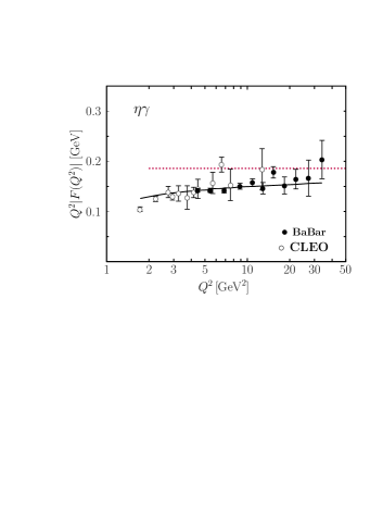
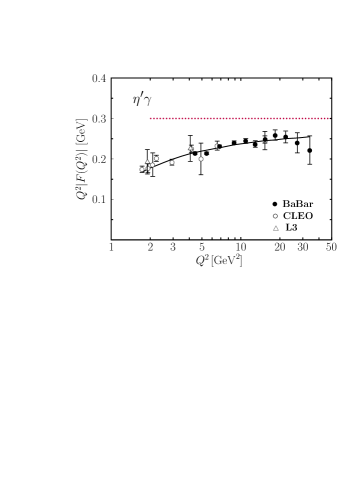
Using this standard setting together with the mixing parameters derived in [39], we fit the Gegenbauer coefficients of order 2 to the data 555 The signs of the transition form factors are not measured. 666The CLEO collaboration [8] measured the form factors for various decay channels. We take into account all of them. In cases where for a given value of there are several values of the form factor we use their error-weighted average. 777Above there is only one data point from [9] with a large error. It has no bearing on our fits and will therefore be not mentioned explicitly in the following. [2, 8]. The result of this fit, termed the default fit in the following, is quoted in Tab. 2 and shown in Fig. 2. For comparison the results of fits to only the CLEO data [8] and only the BaBar data [2] are also shown in Tab. 2. The latter fit can be regarded as a change of the minimal value of for which data are taken into account in the fits.
One notices that the three sets of parameters for the quark distribution amplitudes agree quite well with each other. Deviations of a little more than are seen for . The effect of the Babar data in combination with the CLEO one results in a reduction of the parameter errors and a more precise determination of . In contrast to our previous work where we have had at disposal only the CLEO data [8] and have chosen and , the gluon distribution amplitude is not compatible with zero now. The reasonable agreement of the three fits demonstrates the consistency of the CLEO [8] and BaBar data [2]. The of the default fit is very good given that all together 40 data points are included in the fit. In Fig. 2 the fit is compared to experiment.
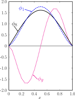
The distribution amplitudes corresponding to the default fit (see Tab. 2) are shown in Fig. 3. Those for the octet and singlet components are close to the asymptotic form of a meson distribution amplitude. They are symmetric around while the gluon distribution amplitude is antisymmetric. We repeat that the distribution amplitudes are to be considered as effective ones since the parameters are contaminated by higher order Gegenbauer coefficients.
4.1.1 Scale dependence
Let us discuss the scales dependence in more detail. In principle, renormalization and factorization scales can be chosen independently. In this work we have chosen for the default fit but we also investigate other choices of the scales in order to learn about the theoretical uncertainties of our results.
For the renormalization scale the usual choice is . On the basis of a next-next-to-leading order calculation of the pion transition form factor it has been argued in [54, 53] that another possible choice of is the square root of the average virtuality instead of the characteristic scale of the process, . For the transition form factors the average virtuality is . Hence, in order to explore the renormalization scale dependence of the resulting distribution amplitudes we also utilize this choice. As an inspection of Tab. 2 reveals the dependence of the fit on the renormalization scale is rather strong; the change of from to results in substantial change of the parameters although both the fits are of similar quality. Thus, the theoretical uncertainties of our results are larger than indicated by the errors of the fitted Gegenbauer coefficients.
It is important to note that our NLO calculation is in fact the LO calculation in and it is a well known fact that in order to stabilize the dependence on the NLO QCD corrections i.e., NNLO corrections to the transition form factor, should be included. At NNLO the presence of terms stabilizes the dependence on and all predictions fall relatively close (see, for example, [55] for discussion on that point). Concerning fits, one would thus expect that the inclusion of NNLO would considerably decrease the variation of the obtained Gegenbauer coefficients with . Without this stabilizing effect of NNLO we are left with the variation illustrated in Tab. 2. We note that in order to circumvent this scale ambiguity one can claim to have found a sensible renormalization scale setting a number of which has been proposed in the literature (see Ref. [56] and references therein) as, for example, the principle of maximum conformality where all non-conformal terms associated with the -function in the perturbative series are summed into the running coupling and a scale-fixed prediction is obtained.
Next, we turn to the factorization scale choice. As elaborated in [53], the dependence on can be cancelled order by order in by performing the resummation of terms up to the characteristic scale of the (one-scale) process , and this turns out to be an equivalent of the choice . Still, to test the strength of the residual dependence of the expression (19) on the factorization scale we perform a fit with the choice . From the results, quoted in Tab. 2, one sees that the fit mildly depends on . The quark Gegenbauer coefficients hardly change. For the factorization scale dependence is a bit more pronounced although the values of agree within errors for the two fits with different but the same renormalization scale.
4.1.2 Parameter correlations and evolution of Gegenbauer coefficients
| Scales | |||
|---|---|---|---|
| 0.371 | 0.248 | 0.057 | |
| 0.607 | 0.228 | 0.057 | |
| 0.760 | 0.202 | 0.058 |
The parameter correlations offer an additional quantitative and qualitative insight into our fits so we present them here, as well as, comment on the general behavior of the Gegenbauer coefficients under evolution.
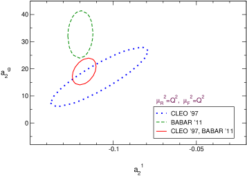
Due to mixing under evolution we expect the strongest correlation between the Gegenbauer coefficients and . Inspection of Fig. 4 reveals that the correlation is particularly strong for the fit to just the CLEO data but becomes milder for the fit to the combined CLEO and BaBar data. This goes parallel with a reduction of the parameter errors. The strength of the correlation between and depends on the chosen factorization and renormalization scales; it is smallest for the standard setting, see Tab. 3 where we compile the correlation coefficients for the three fits to the CLEO and BaBar data. So the higher the scales, the lower are the correlations between and . Furthermore, the correlation between and is mild while and are nearly uncorrelated. The origin of the correlation between and the other Gegenbauer coefficients lies in mixing. The form factor is dominated by the octet contribution () while is mainly fed by the singlet one ().
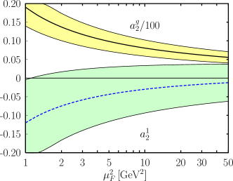
The evolution of the Gegenbauer coefficients and is shown on the right hand side of Fig. 4. The coefficients decrease relatively fast from the initial scale, up to about GeV2 and after that the approach to zero is slow. This behavior is a consequence of the properties of the logarithm contained in (see (2)): for (in fact for ) the derivative of the logarithm is very small. The Gegenbauer coefficients of the octet distribution amplitude evolve similarly. This flat behavior of the logarithm for large scales is also partially responsible for the fact that even in a NLO calculation one can determine only one Gegenbauer coefficient for each distribution amplitude or, more precisely, one linear combination of them.
4.1.3 OZI rule constraints
The opposite Fock components from Eqs. (12-13) lead to violations of the OZI rule if they were not suppressed. Hence, one expects that
| (21) |
holds for any values of at least for a limited range of the factorization scale. Asymptotically, where all distribution amplitudes evolve in , is zero anyway. To a sufficient degree of accuracy (21) can be replaced by
| (22) |
Indeed, as can be seen from Table 2, the default fit meets (22) at the initial scale and, as can readily be checked, at all larger factorization scales: . Hence, no substantial violations of the OZI rule follow from the distribution amplitudes specified by the default fit and shown in Figs. 3. Also the fits using different choices of and as well as those to just the CLEO or BaBar data satisfy (22).
In order to avoid large violations of the OZI rule one may follow a suggestion made in [26] and assume at the initial scale. Although evolution generates some violations of the OZI rule with increasing scale they are always sufficiently small. The fit assuming and using the mixing parameters of [39, 40] is still of reasonable quality. Although is somewhat larger, the fit parameters are similar to those obtained from the three-parameter fit, see Tab. 2. The difficulties with the OZI rule of the mixing parameters determined in [44] (see Tab. 1) is corroborated by the analogous fit with . This fit fails badly, is 240.
Let us end with some additional comments on various mixing parameters from the literature in the context of OZI rule violations. Using the mixing parameters determined in [44] which markedly differ from those given in [39, 40], one also arrives at a reasonable fit to the form factor data with regard to . However, in this case is positive leading to rather large OZI rule violations. The mixing parameters given in [44] are therefore to be employed with reservation. It is to be mentioned that the work [44] has also been criticized in [15] on the basis of an analysis of the transition form factors with a -anomaly sum rule. The theoretical set of mixing parameters discussed in [43] is intermediate between [39, 40] and [44]. The quality of the fit to the form factor data is similar to other fits but the difference is rather large although smaller than for the fit using the mixing parameters given in [44]. Thus, with regard to the strength of OZI rule violation the mixing parameters given in [39, 40] seem to be favored. Ideally one should fit the mixing parameters together with the lowest Gegenbauer coefficients to the data. Unfortunately such a multi-parameter fit does not lead to a reasonable solution, there are extremely strong correlations among the parameters, often large violations of the OZI rule and a covariance matrix that is not positive definite. Thus, we refrain from discussing such fits.
4.2 Comparison to other results
We here briefly discuss our results in relation to some relevant results found in the literature.
Ali and Parkhomenko [18] have performed an analysis of the energy spectrum in the inclusive decay [57] in order to constrain the -meson distribution amplitude. At an intermediate step of the analysis of the energy spectrum the transition form factor is to be calculated (see Sect. 6). From the high end of the meson energy spectrum Ali and Parkhomenko determine the Gegenbauer coefficients and which are in agreement with our results within very large errors. In order to calculate the energy spectrum also at low and even negative gluon virtualities Ali and Parkhomenko introduce a positivity constraint for the transition form factor which is achieved by choosing . This constraint significantly reduce the allowed range for the Gegenbauer coefficients and, in combination with our previous result [6] they obtain
| (23) |
at the initial scale . While the value for agrees with our default result within errors, our result for the coefficient is larger as a consequence of the BaBar data which were not available to the authors of [18]. The role of the positivity constraint used in [18] remains to be understood.
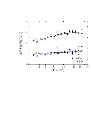
The lowest Gegenbauer coefficient of the octet distribution amplitude has been calculated with the help of QCD sum rules in Ref. [58]. A value of about with a large uncertainty has been obtained for the coefficient . In this calculation the distribution amplitude is normalized to . For the larger octet decay constant (see Tab. 1) we are using the value of is expected to be somewhat smaller, say, about 0.16. Given the large uncertainty of the sum rule result this value is not in conflict with our default fit. However this large face value of the sum rule result can only be reconciled with the form factor data if one allows for an additional power correction (or for higher Gegenbauer coefficients) which compensate the positive to a large extent. In order to examine this possibility we extract the octet contribution to the transition form factors using (17), and (10)
| (24) |
and perform a fit analogously to the ones described above but allowing for an additional power correction to it. Keeping fixed and using the mixing parameters determined in [39, 40], we obtain from the fit to the data on . For the 15 data points the minimum is 21 which is somewhat larger than our best result ( for , ) but still tolerable. Freeing also a very good fit is obtained (, , ). The latter fit is shown in Fig. 5 and compared to experiment. In this figure also the results of the default fit for the octet and singlet form factors
| (25) |
are displayed and compared with experiment.
4.3 A comment on the time-like data
The BaBar collaboration [27] has measured the and transition form factors at . We do not include these data in our analysis since the theoretical treatment of form factors in the time-like region is non-trivial and not well understood. In the time-like region the form factors are no longer real and there are subtleties regarding the analytic continuation from the space- to the time-like region [59] (and references therein).
Compared with the naive expectation that at the form factor should be close to the asymptotic prediction the Babar result for the form factor is about too large. This discrepancy is likely not a consequence of the description of mixing. The quark-flavor mixing scheme is on sound theoretical grounds and is phenomenologically well established in a large variety of processes. A discrepancy for a single data point cannot discard this mixing scheme. In contrast to the case of the the form factor at measured by the BaBar collaboration [27], is in agreement with the naive expectation.
4.4 The vertex
We are now in the position to repeat the evaluation of the form factors we performed in [6]. With the results on the gluon distribution amplitude obtained from the present analysis of the transition form factors we believe to have more precise results for the form factors now. On the importance of these form factors we have already commented in the introduction.
The gluonic vertex is written analogously to the electromagnetic one as
| (26) |
where and now denote the momenta of the gluons and and label the color of the gluon.
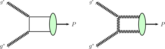
According to [6] the transition form factor to leading-twist accuracy and lowest order of is to be calculated from Feynman graphs of which examples are shown in Fig. 6.
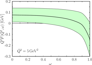
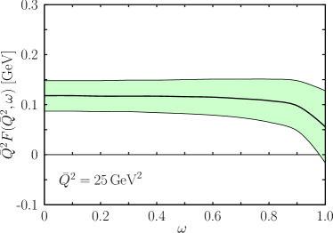
The results are given in [6] and are not repeated here. Using the Gegenbauer coefficients of the default fit, we can readily evaluate the transition form factor. The results, including the error band, are shown in Fig. 7 for two values of . As compared to our previous results [6] the error bands are markedly narrower while the central values do not differ much.
As for the and transition form factors and in order to be consistent with that analysis power corrections are neglected here as well. For the vertex function, in particular for , any power corrections as for instance quark transverse momenta or meson mass corrections, are small since the vertex function is not end-point sensitive in this kinematic limit. Mass corrections to the vertex function have been estimated by Ali and Parkhomenko [18, 19].
5 The transition form factor
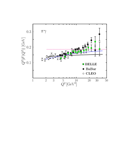
Finally, we present the preliminary analysis and discussion of the transition form factor which is inspired by the availability of both [2] and [4] data.
For comparison we show in Fig. 8 the data on the transition form factor [2, 4, 8]. It is important to realize the dramatic difference between the BaBar data [2] on the form factor and the data. In contrast to the latter a leading-twist analysis of the form factor to fixed order of perturbative QCD fails because the data do not seem to respect dimensional scaling. Power corrections seem to be demanded by the data as well as a positive value of the 2nd Gegenbauer coefficient of the pion distribution amplitude, see for instance [10, 16, 38]. This difference between the and the other form factors implies a strong breaking of flavor symmetry which has never been observed in the sector of pseudoscalar mesons before.
On the other hand, the BELLE data [4] do not show this sharp rise with , they lie systematically below the BaBar data. They do not exceed the asymptotic result for the form factor and are close to the behavior of the NLO leading-twist approach as is the case of the other transition form factors. An example of such a fit to the data from [8] and [4] is shown in Fig. 8 (with and for 28 data points). Although the of this fit is reasonable the dependence of the fit seems to be too flat as compared to the BELLE data which may be viewed as a hint at lacking power corrections. For instance, a result obtained with factorization which encodes corrections of order , is in good agreement with the CLEO and BELLE data [31]. We finally emphasize that the BELLE data imply only mild violations of flavor symmetry. A more detailed comparison of the BaBar and BELLE data with theoretical models can be found in [64]. Although the BELLE data seem to be favored against the BaBar data with regard to the standard theoretical concepts, an understanding of the origin of the discrepancy between the two measurements is required.
6 Summary
We have analyzed the and transition form factors within a collinear factorization approach to leading-twist accuracy and NLO of perturbative QCD. The analysis of the data [2, 8] allowed for an extraction of the lowest Gegenbauer coefficients of the flavor-octet and singlet distribution amplitudes as well as that of the glue-glue distribution amplitude. The Gegenbauer coefficients are better determined now and have smaller errors than those extracted in [6]. Our default result for is (see Tab. 2):
| (27) |
There are a number of uncertainties of this result. First there is the uncertainty due to the chosen renormalization scale. Next, despite the large range of covered by data now one still cannot determine more than the lowest Gegenbauer coefficients of the three distribution amplitudes. The coefficients we quote are to be regarded as effective parameters which are contaminated by higher order Gegenbauer coefficients. In fact, according to the discussion at the end of Sect. 4.1.2, it seems impossible to extract more information from the transition form factors than the lowest Gegenbauer coefficients. In order to determine more Gegenbauer coefficients additional processes have to be analyzed. Finally, given the quality of the present data, it is still not possible to discriminate between the logarithmic dependence generated by the evolution and the NLO corrections, and power corrections (see the discussion in Sect. 4.2). We have neglected power correction in our analysis. Allowing for power corrections in the form factor analysis one may for instance find positive Gegenbauer coefficients as is the case for the pion distribution amplitude (e.g. [38]).
As an application of our results for the Gegenbauer coefficients we calculated the vertex function. Another processes in which the gluon-gluon Fock components of the and mesons may play an important role, are the () decays into pairs of and/or mesons. Here, the -quark mass is considered to be large enough to allow for a perturbative treatment of these decays. An explicit calculation of the perturbative contribution to the decays taking into account the two-gluon Fock components, is tedious, many Feynman graphs contribute even to lowest order [60]. Moreover, there is another complication. As is shown in [61] the next higher Fock state, , of the , the so-called color-octet contribution [62], is also to be taken into account since it scales with the same power of the hard scale, , as the contribution. With regard to these complications whose detailed calculation is very time-consuming, we will not attempt a complete analysis of these decay processes; this is beyond the scope of the present paper. A statement whether or not our distribution amplitudes are in conflict with the peculiar features of the decays [49, 52, 63] is therefore premature.
This work was supported in part by the BMBF under the contract No. 06RY9191 and in part by Croatian Ministry of Science, Education and Sport under the contract no. 098-0982930-2864.
References
- [1] B. Aubert et al. [The BABAR Collaboration], Phys. Rev. D 80, 052002 (2009) [arXiv:0905.4778 [hep-ex]].
- [2] P. del Amo Sanchez et al. [BABAR Collaboration], Phys. Rev. D 84, 052001 (2011) [arXiv:1101.1142 [hep-ex]].
- [3] G. P. Lepage and S. J. Brodsky, Phys. Lett. B 87, 359 (1979).
- [4] S. Uehara et al. [Belle Collaboration], arXiv:1205.3249 [hep-ex].
- [5] T. Feldmann and P. Kroll, Eur. Phys. J. C 5, 327 (1998) [hep-ph/9711231].
- [6] P. Kroll, K. Passek-Kumericki, Phys. Rev. D67, 054017 (2003). [hep-ph/0210045].
- [7] S. S. Agaev, N. G. Stefanis, Phys. Rev. D70, 054020 (2004). [hep-ph/0307087].
- [8] J. Gronberg et al. [CLEO Collaboration], Phys. Rev. D 57, 33 (1998) [hep-ex/9707031].
- [9] M. Acciarri et al. [L3 Collaboration], Phys. Lett. B 418, 399 (1998).
- [10] P. Kroll, Eur. Phys. J. C71, 1623 (2011). [arXiv:1012.3542 [hep-ph]].
- [11] T. Huang and X. -G. Wu, Int. J. Mod. Phys. A 22 (2007) 3065 [hep-ph/0606135].
- [12] X. -G. Wu and T. Huang, Phys. Rev. D 84 (2011) 074011 [arXiv:1106.4365 [hep-ph]].
- [13] S. J. Brodsky, F. -G. Cao, G. F. de Teramond, Phys. Rev. D 84, 075012 (2011) [arXiv:1105.3999 [hep-ph]].
- [14] A. E. Dorokhov, A. E. Radzhabov, A. S. Zhevlakov, Eur. Phys. J. C 71, 1702 (2011) [arXiv:1103.2042 [hep-ph]].
- [15] Y. N. Klopot, A. G. Oganesian, O. V. Teryaev, Phys. Rev. D 84, 051901 (2011) [arXiv:1106.3855 [hep-ph]].
- [16] D. Melikhov and B. Stech, arXiv:1202.4471 [hep-ph].
- [17] S. Noguera and S. Scopetta, arXiv:1110.6402 [hep-ph].
- [18] A. Ali, A. Y. Parkhomenko, Eur. Phys. J. C30, 183 (2003). [hep-ph/0304278].
- [19] A. Ali, A. Y. Parkhomenko, Eur. Phys. J. C30, 367-380 (2003). [arXiv:hep-ph/0307092 [hep-ph]].
- [20] L. A. Harland-Lang, V. A. Khoze, M. G. Ryskin, W. J. Stirling, Eur. Phys. J. C 71, 1714 (2011) [arXiv:1105.1626 [hep-ph]].
- [21] M. Gronau and J. L. Rosner, Phys. Rev. D 53, 2516 (1996)
- [22] M. Beneke, M. Neubert, Nucl. Phys. B675, 333-415 (2003). [hep-ph/0308039].
- [23] A. R. Williamson, J. Zupan, Phys. Rev. D74, 014003 (2006). [hep-ph/0601214].
- [24] J. Schumann et al. [ Belle Collaboration ], Phys. Rev. Lett. 97, 061802 (2006). [hep-ex/0603001].
- [25] B. Aubert et al. [ The BABAR Collaboration ], Phys. Rev. D80, 112002 (2009). [arXiv:0907.1743 [hep-ex]].
- [26] P. Ball, G. W. Jones, JHEP 0708, 025 (2007). [arXiv:0706.3628 [hep-ph]].
- [27] B. Aubert et al. [BABAR Collaboration], Phys. Rev. D 74, 012002 (2006) [hep-ex/0605018].
- [28] M. V. Terentev, Sov. J. Nucl. Phys. 33, 911 (1981) [Yad. Fiz. 33, 1692 (1981)].
- [29] V. N. Baier and A. G. Grozin, Nucl. Phys. B 192, 476 (1981).
- [30] D. Müller, Phys. Rev. D 51, 3855 (1995) [hep-ph/9411338].
- [31] P. Kroll and M. Raulfs, Phys. Lett. B 387, 848 (1996) [hep-ph/9605264].
- [32] G. P. Lepage and S. J. Brodsky, Phys. Rev. D 22, 2157 (1980).
- [33] J. B. Kogut and D. E. Soper, Phys. Rev. D 1, 2901 (1970).
- [34] R. Kaiser and H. Leutwyler, Eur. Phys. J. C 17, 623 (2000) [hep-ph/0007101].
- [35] A. V. Belitsky and D. Mueller, Nucl. Phys. B 537, 397 (1999) [hep-ph/9804379].
- [36] F. del Aguila and M. K. Chase, Nucl. Phys. B 193, 517 (1981);
- [37] E. Braaten, Phys. Rev. D 28, 524 (1983);
- [38] S. S. Agaev, V. M. Braun, N. Offen, F. A. Porkert, Phys. Rev. D83, 054020 (2011). [arXiv:1012.4671 [hep-ph]].
- [39] T. Feldmann, P. Kroll, B. Stech, Phys. Rev. D58, 114006 (1998). [hep-ph/9802409].
- [40] T. Feldmann, P. Kroll, B. Stech, Phys. Lett. B449, 339-346 (1999). [hep-ph/9812269].
- [41] F. De Fazio, M. R. Pennington, JHEP 0007, 051 (2000). [hep-ph/0006007].
- [42] E. B. Gregory, A. C. Irving, C. M. Richards and C. MacNeile [UKQCD collaboration], arXiv: 1112.4384 [hep-lat].
- [43] P. Kroll, Mod. Phys. Lett. A20, 2667-2684 (2005). [hep-ph/0509031].
- [44] R. Escribano, J. -M. Frere, JHEP 0506, 029 (2005). [hep-ph/0501072].
- [45] J. L. Goity, A. M. Bernstein, B. R. Holstein, Phys. Rev. D66, 076014 (2002). [hep-ph/0206007].
- [46] J. Schechter, A. Subbaraman, H. Weigel, Phys. Rev. D48, 339-355 (1993). [hep-ph/9211239].
- [47] T. Huang and X. -G. Wu, Eur. Phys. J. C 50, 771 (2007) [hep-ph/0612007].
- [48] C. Di Donato, G. Ricciardi, I. Bigi, Phys. Rev. D 85, 013016 (2012) [arXiv:1105.3557 [hep-ph]].
- [49] C. E. Thomas, JHEP 0710, 026 (2007). [arXiv:0705.1500 [hep-ph]].
- [50] V. Crede, C. A. Meyer, Prog. Part. Nucl. Phys. 63, 74-116 (2009). [arXiv:0812.0600 [hep-ex]].
- [51] M. Diehl, P. Kroll, C. Vogt, Eur. Phys. J. C22, 439-450 (2001). [hep-ph/0108220].
- [52] K. Nakamura et al. [ Particle Data Group Collaboration ], J. Phys. G G37, 075021 (2010).
- [53] B. Melić, B. Nižić and K. Passek, Eur. Phys. J. C 36, 453 (2004) [arXiv:hep-ph/0107311 [hep-ph]].
- [54] B. Melić, B. Nižić and K. Passek, Phys. Rev. D 65, 053020 (2002) [hep-ph/0107295].
- [55] B. Melić, B. Nižić and K. Passek, Phys. Rev. D 60, 074004 (1999) [hep-ph/9802204].
- [56] X. -G. Wu, S. J. Brodsky and M. Mojaza, arXiv:1302.0599 [hep-ph].
- [57] M. Artuso et al. [CLEO Collaboration], Phys. Rev. D 67, 052003 (2003) [hep-ex/0211029].
- [58] P. Ball, JHEP 9901, 010 (1999). [hep-ph/9812375].
- [59] A. P. Bakulev, A. V. Radyushkin and N. G. Stefanis, Phys. Rev. D 62, 113001 (2000) [hep-ph/0005085].
- [60] V.N. Baier and A.G. Grozin, Z. Phys. C29, 161 (1985).
- [61] J. Bolz, P. Kroll and G. A. Schuler, Eur. Phys. J. C 2, 705 (1998) [hep-ph/9704378].
- [62] G. T. Bodwin, E. Braaten and G. P. Lepage, Phys. Rev. D51 (1995) 1125.
- [63] H. -B. Li [ BESIII Collaboration ], PoS FPCP2010, 004 (2010). [arXiv:1101.2049 [hep-ex]].
- [64] A. P. Bakulev, S. V. Mikhailov, A. V. Pimikov and N. G. Stefanis, arXiv:1205.3770 [hep-ph].