Dielectric function, screening, and plasmons of graphene in the presence of spin-orbit interactions

Abstract

We study the dielectric properties of graphene in the presence of Rashba and intrinsic spin-orbit interactions in their most general form, i.e., for arbitrary frequency, wave vector, doping, and spin-orbit coupling (SOC) parameters. The main result consists in the derivation of closed analytical expressions for the imaginary as well as for the real part of the polarization function. Several limiting cases, e.g., the case of purely Rashba or purely intrinsic SOC, and the case of equally large Rashba and intrinsic coupling parameters are discussed. In the static limit the asymptotic behavior of the screened potential due to charged impurities is derived. In the opposite limit ($q=0$, $\omega\to 0$), an analytical expression for the plasmon dispersion is obtained and afterwards compared to the numerical result. Our result can also be applied to related systems such as bilayer graphene or topological insulators.

I Introduction

It is now well established that at low energies the charge carriers in graphene are described by a Dirac-like equation for massless particles.Wallace ; CastroNetoRMP09 While standard graphene, i.e., without any spin-orbit interactions (SOIs), does not exhibit a band gap, a gap opens up in the spectrum if one includes purely intrinsic spin-orbit interactions.Kane_2005 The corresponding energy dispersion resembles that of a massive relativistic particle with a rest energy which is proportional to the spin-orbit coupling parameter (SOC). Including SOIs of the Rashba type, e.g., by applying an external electric field, lifts the spin degeneracy. Depending on the ratio of the intrinsic and the Rashba parameters a gap can occur in the spectrum or not.

Many theoretical studies on the dielectric function of various systems have been made in the last years. Besides semiconductor two-dimensional electron gasesPletyuhkov_2006 ; Badalyan_2010 ; Ullrich_2003 and hole gas systems,Schliemann_2010 large investigations have been made in graphene. Starting from the simplest possible graphene model within the Dirac-cone approximation,Wunsch ; Sarma ; Polini more and more extensions have been included. These extensions range from numericalStauber_2010 ; Stauber_2010_2 and analyticalStauber_2010_3 tight-binding studies and the inclusion of a finite band gap Pyat ; Wang_2007_2 ; Scholz_2011 to double- and multilayer graphene samples,Borghi_2009 ; Gamayun_2011 ; Yuan_2011 ; Stauber_2012 ; Profumo_2012 ; Triola_2012 graphene antidot lattices,Schultz_2011 and graphene under a circularly polarized ac electric field.Busl_2011

In this work we study the dielectric properties of graphene including both the Rashba and the intrinsic spin-orbit coupling. While the case of purely intrinsic interactions is well understood,Pyat ; Wang_2007_2 ; Scholz_2011 the dielectric function for the general case, where both types of SOIs are present, is unknown. Other previous studies have investigated the effect of SOI on magnetotransport Ding_2008 and the optical conductivity.Ingenhoven_2010 ; Hill_2011

Our study is motivated by recent experimental and theoretical works demonstrating that the SOC parameters can significantly be enlarged by choosing proper adatoms Neto09 ; Weeks_2011 ; Ma_2012 or a suitable environment.Dedkov_2008 ; Varykhalov_2008 ; Jin_2012

Information that can be extracted from the dielectric function range from the screening between charged particles to the collective charge excitations formed due to the long-ranged Coulomb interaction. Knowledge of the latter is not only important for possible future applications in the field of plasmonics, where graphene seems to be a promising material,Plasmonics but also because of fundamental reasons. Recent experiments and theoretical studies showed that interactions between charge carriers and plasmons in graphene, forming so-called plasmarons, yield to measurable changes in the energy spectrum.Bostwock_2010

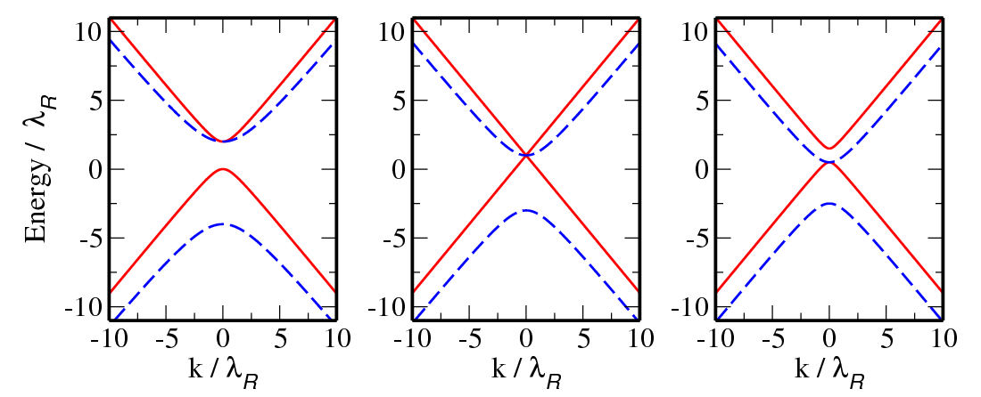
Figure 1: Energy dispersion in units of $\lambda_{R}$ for $E_{+\pm}$ (solid lines) and $E_{-\pm}$ (dashed lines): (a) $\lambda_{I}=2\lambda_{R}$, (b) $\lambda_{I}=\lambda_{R}$, (c) $\lambda_{I}=\lambda_{R}/2$.

The paper is organized as follows. In Sec. II, we introduce the model Hamiltonian including the eigensystem and summarize the formalism of the random phase approximation (RPA). In Sec. III, analytical and numerical results for the free polarization function of the undoped and the doped system are given. In Sec. IV, the dielectric function is used to analyze the static screening properties due to charged impurities. We provide qualitatively the asymptotic behavior of the induced potential. The long-wavelength collective charge excitations of graphene are derived in Sec. V and afterwards compared to the numerical result. We find the existence of several new potential plasmon modes that are absent without any spin-orbit interactions. Most of these zeros, however, are overdamped as can be seen from the energy loss function. We close with conclusions and outlook in Sec. VI. Finally, in Appendixes A and B we give details of the calculation of the free polarization function.

II The model

We describe graphene with SOI within the Dirac cone approximation. At one $K$ point, the Hamiltonian is given by Kane_2005

$$\hat{H}=v_{F}\boldsymbol{p}\cdot\boldsymbol{\tau}+\lambda_{R}\left(\boldsymbol{\tau}\times\boldsymbol{\sigma}\right)\boldsymbol{e}_{z}+\lambda_{I}\tau_{z}\sigma_{z}.$$ (1)

The Pauli matrices $\boldsymbol{\tau}$ ($\boldsymbol{\sigma}$) act on the pseudospin (real spin) space. The other $K$ point can be described by the above Hamiltonian with $\sigma_{x}\rightarrow-\sigma_{x}$ and $\sigma_{z}\rightarrow-\sigma_{z}$. Since the two $K$ points are not coupled, we can limit our discussion to the above Hamiltonian, multiplying the final results by the valley index $g_{v}=2$. Moreover, without loss of generality, we assume a positive Rashba and intrinsic coupling as the eigensystem and thus the dielectric function is not changed for negative values.

II.1 Solution

For a sufficiently large intrinsic coupling parameter, $\lambda_{I}>\lambda_{R}$, the system is in the spin quantum Hall phase with a characteristic band gap. For $\lambda_{R}>\lambda_{I}$ the gap in the spectrum is closed and the system behaves as an ordinary semimetal. At the point where $\lambda_{R}=\lambda_{I}$ a quantum phase transitions occurs in the system. In the following we mainly set $v_{F}=1$ and $\hbar=1$.

The eigensystem reads

$$\left|\chi_{\pm\pm}(\boldsymbol{k})\right\rangle=\frac{1}{\sqrt{2}}\begin{pmatrix}\sin{\left(\theta_{\mp}/2\right)}\\ \cos{\left(\theta_{\mp}/2\right)}e^{i\varphi}\\ \pm\cos{\left(\theta_{\mp}/2\right)}e^{i\varphi}\\ \pm\sin{\left(\theta_{\mp}/2\right)}e^{2i\varphi}\end{pmatrix},$$

$$\left|\chi_{\pm\mp}(\boldsymbol{k})\right\rangle=\frac{1}{\sqrt{2}}\begin{pmatrix}\cos{\left(\theta_{\mp}/2\right)}\\ -\sin{\left(\theta_{\mp}/2\right)}e^{i\varphi}\\ \mp\sin{\left(\theta_{\mp}/2\right)}e^{i\varphi}\\ \pm\cos{\left(\theta_{\mp}/2\right)}e^{2i\varphi}\end{pmatrix},$$ (2)

with $\sin{(\theta_{\pm})}=\frac{k}{\sqrt{k^{2}+\lambda_{\pm}^{2}}}$ and $\lambda_{\alpha}=\lambda_{R}+\alpha\lambda_{I}$, and ($k=\left|\boldsymbol{k}\right|$)

$$E_{\alpha\beta}(\boldsymbol{k})=\alpha\;\lambda_{R}+\beta\;\sqrt{k^{2}+{\lambda_{-\alpha}}^{2}}\quad(\alpha,\beta=\pm 1).$$ (3)

For $\lambda_{R}\neq 0$ the spin degeneracy is lifted and two distinct Fermi wave vectors, $k_{F\pm}=\sqrt{\mu\left(\mu\mp 2\lambda_{R}\right)\pm 2\lambda_{R}\lambda_{I}-\lambda_{I}^{2}}$, exist. In Fig. 1, the energy dispersion is shown for three characteristic values of the SOI.

The energy scales for the SOC parameters in monolayer graphene, $\lambda_{I}=12\mu{\rm eV}$ and $\lambda_{R}=5\mu{\rm eV}$ for an electric field of $1{\rm\frac{V}{nm}}$, are generally small Gmitra_2009 . However, it was shown that these parameters can be enlarged to $\lambda_{I}\approx 30{\rm meV}$ for thallium adatoms Weeks_2011 or $\lambda_{R}\approx 13\rm{meV}$ for graphene placed on a Ni(111) surface.Varykhalov_2008

The above Hamiltonian with only Rashba coupling can be mapped onto the bilayer Hamiltonian without SOI, relating the interlayer hopping parameter $t_{IL}\approx 0.2{\rm eV}$ Min_2007 to the Rashba SOC. Our findings can also be applied to a topological insulator within the Kane-Mele model.Kane_2005

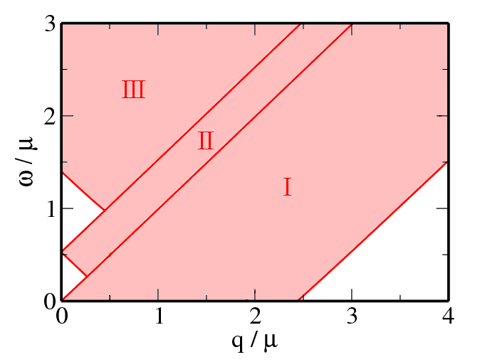
Figure 2: Single-particle continuum (dark area) for the particular choice of $\lambda_{R}=2\lambda_{I}=0.3\mu$. Analytical expressions for the boundaries of the distinct regions I, II and III can be found in Sec. III B.

II.2 Dielectric function

In order to find the dielectric function in RPA Guil given by

$$\varepsilon(q,\omega)=1-V(q)\chi_{0}(q,\omega),$$ (4)

where $V(q)=\frac{e^{2}}{2\epsilon_{0}q}$ is the Fourier transform of the Coulomb potential in two dimensions, $V(r)=\frac{e^{2}}{4\pi\epsilon_{0}r}$, and $\epsilon_{0}$ the vacuum permittivity, one needs to calculate the free polarization,

$$\chi_{0}(q,\omega)=\sum_{\alpha,\eta_{i}=\pm 1}\int\frac{g_{v}d^{2}k}{(2\pi)^{2}}\left|\left\langle\chi_{\eta_{1}\eta_{2}}\left(\boldsymbol{k}\right)\bigg{|}\chi_{\eta_{3}\eta_{4}}\left(\boldsymbol{k}+\boldsymbol{q}\right)\right\rangle\right|^{2}$$

$$\times\frac{\alpha\,f(E_{\eta_{1}\eta_{2}}(\boldsymbol{k}))}{\omega-\alpha\left[E_{\eta_{3}\eta_{4}}\left(\boldsymbol{k}+\boldsymbol{q}\right)-E_{\eta_{1}\eta_{2}}\left(\boldsymbol{k}\right)\right]+i0}.$$ (5)

In the following we assume zero temperature. The Fermi function $f(E)$ then reduces to a simple step function. Because of the general relation $\chi_{0}(q,-\omega)=\left[\chi_{0}(q,\omega)\right]^{*}$, we restrict our discussions to positive frequencies $\omega$.

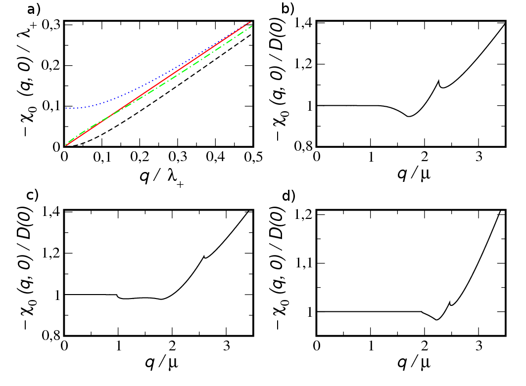
Figure 3: Static real part of the charge susceptibility for (a) undoped graphene with fixed $\lambda_{+}$ for $\lambda_{R}=2\lambda_{I}$ (dotted), $\lambda_{R}=\lambda_{I}$ (dot-dashed), $\lambda_{I}=2\lambda_{R}$ (dashed), $\lambda_{R}=\lambda_{I}=0$ (straight), and doped graphene with (b) $\lambda_{R}=\lambda_{I}=0.3\mu$, (c) $\lambda_{R}=2\lambda_{I}=0.3\mu$, and (d) $2\lambda_{R}=\lambda_{I}=0.3\mu$ in units of the density of states $\rm{D}(0)=g_{v}\mu/\pi$.

III Analytical results

III.1 Zero doping

For zero doping the valence bands are completely filled while the conduction bands are empty. Only transitions between bands $E_{\alpha-}$ and $E_{\beta+}$ are possible. The resulting charge correlation function can be decomposed as

$$\bar{\chi}_{0}(q,\omega)=\sum_{\eta_{i}=\pm}\chi^{\eta_{1}-\to\eta_{3}+}(q,\omega)$$ (6)

Here we introduced the notation $\chi^{\eta_{1}\eta_{2}\to\eta_{3}\eta_{4}}(q,\omega)$ describing transitions from the initial band $E_{\eta_{1}\eta_{2}}(\boldsymbol{k})$ to the final band $E_{\eta_{3}\eta_{4}}(\boldsymbol{k}+\boldsymbol{q})$. For the imaginary part we find

$$\operatorname{Im}\left\{\chi^{\mp-\to\mp+}(q,\omega)\right\}=\frac{g_{v}}{16}\;\theta\left[\omega^{2}-q^{2}-4{\lambda_{\pm}}^{2}\right]$$

$$\quad\times\left[\frac{3q^{4}-4{\lambda_{\pm}}^{2}q^{2}-5q^{2}\omega^{2}+2\omega^{4}}{\left(\omega^{2}-q^{2}\right)^{3/2}}\right.$$

$$\quad\left.-\frac{\left|q^{2}-\omega\left(\omega-2\lambda_{\pm}\right)\right|+\left|q^{2}-\omega\left(\omega+2\lambda_{\pm}\right)\right|}{\omega}\right]$$ (7)

and

$$\operatorname{Im}\left\{\chi^{\pm-\to\mp+}(q,\omega)\right\}=-\frac{g_{v}}{8}\,\theta\left[\omega_{\pm}^{2}-q^{2}-4\gamma^{2}\right]\times$$ (8)

$$\left[\sqrt{\omega_{\pm}^{2}-q^{2}}-\frac{\left|q^{2}-\omega\left(\omega\pm 2\lambda_{-}\right)\right|}{2\omega}-\frac{\left|q^{2}-\omega\left(\omega\pm 2\lambda_{+}\right)\right|}{2\omega}\,\right]$$

Here we defined $\omega_{\pm}=\omega\pm 2\lambda_{R}$ and $\gamma=\text{max}\{\lambda_{R},\lambda_{I}\}$. For equally large spin-orbit coupling parameters, $\lambda_{R}=\lambda_{I}$, the imaginary part is divergent at the threshold $\omega=q$ but finite otherwise. The divergent part of the polarization is $\chi^{+-\to++}$ as the bands $E_{+\pm}(\boldsymbol{k})$ are linear in momentum.

The real part can be obtained via the Kramers-Kronig relations

$$\operatorname{Re}\left\{\bar{\chi}_{0}(q,\omega)\right\}=\frac{2}{\pi}\mathcal{P}\int_{0}^{\infty}d\omega^{\prime}\frac{\omega^{\prime}\operatorname{Im}\left\{\bar{\chi}_{0}(q,\omega^{\prime})\right\}}{\omega^{\prime 2}-\omega^{2}}.$$ (9)

After carrying out the remaining integration, where it is necessary to keep the principal value, we arrive at

$$\operatorname{Re}\left\{\chi^{\mp-\to\mp+}(q,\omega)\right\}=\frac{g_{v}}{8\pi}\left[-2\lambda_{\pm}+2\sqrt{q^{2}+\lambda_{\pm}^{2}}\left(5q^{2}\omega^{2}+4q^{2}\lambda_{\pm}^{2}-3q^{4}-2w^{4}\right)\operatorname{Re}\left\{\frac{\operatorname{arctan}\left(\frac{\sqrt{q^{2}-\omega^{2}}}{2\lambda_{\pm}}\right)}{\left(q^{2}-\omega^{2}\right)^{3/2}}\right\}\right.$$

$$\left.-\frac{2q^{2}\lambda_{\pm}}{q^{2}-\omega^{2}}+2\lambda_{\pm}\ln{\left|\frac{q^{2}-\omega^{2}+4\lambda_{\pm}^{2}}{\left(\sqrt{q^{2}+\lambda_{\pm}^{2}}+\lambda_{\pm}\right)^{2}-\omega^{2}}\right|}-\frac{\omega^{2}-q^{2}}{2\omega}\ln{\frac{\sqrt{q^{2}+\lambda_{\pm}^{2}}+\lambda_{\pm}+\omega}{\sqrt{q^{2}+\lambda_{\pm}^{2}}+\lambda_{\pm}-\omega}}\right]$$ (10)

and

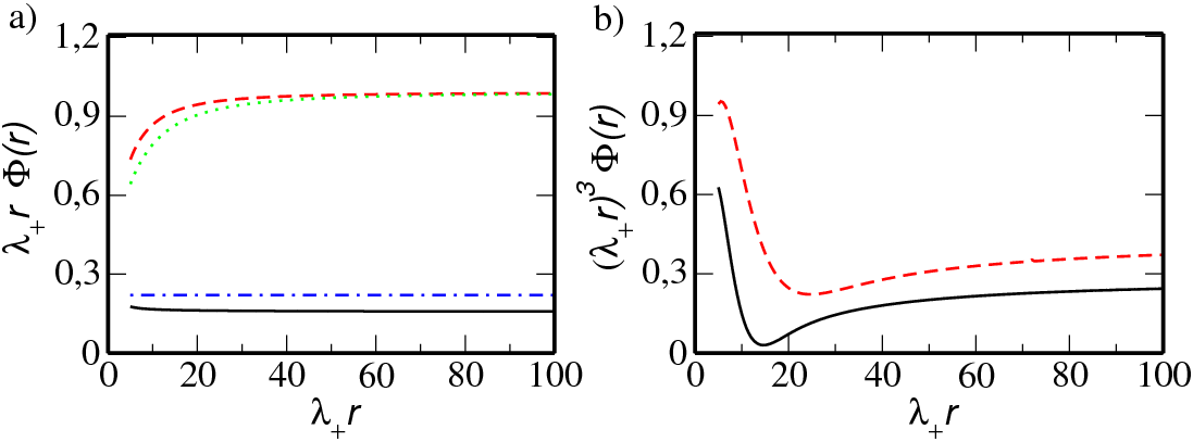
Figure 4: Asymptotic screened potential (in units of $Q\lambda_{+}/\epsilon_{0}$) of undoped graphene for fixed $\lambda_{+}=\lambda_{R}+\lambda_{I}$ and different spin-orbit coupling parameters. (a) $\lambda_{R}=\lambda_{I}$ (straight line), $\lambda_{I}=2\lambda_{R}$ (dashed), $\lambda_{R}=0$ (dotted). Also shown the non-interacting case $\lambda_{R}=\lambda_{I}=0$ (dot-dashed). (b) $\lambda_{I}=0$ (straight), $\lambda_{R}=2\lambda_{I}$ (dashed).

$$\operatorname{Re}\left\{\chi^{\pm-\to\mp+}(q,\omega)\right\}=-\frac{g}{4\pi}\left[2\left(\pm\lambda_{R}-\gamma\pm\lambda_{R}\ln{4}\right)\mp 2\lambda_{R}\operatorname{arcsinh}\left(\frac{2\gamma}{q}\right)\right.$$

$$\left.-\frac{1}{2}\operatorname{Re}\left\{\sqrt{q^{2}-\omega_{\pm}^{2}}\arcsin{\frac{\sqrt{q^{2}-\omega_{\pm}^{2}}\left[q+\omega_{\pm}\left(2\gamma-\sqrt{q^{2}+4\gamma^{2}}\right)\right]}{\sqrt{q^{2}+4\gamma^{2}}-\omega_{\pm}}}\right\}\right.$$

$$\left.-\frac{1}{2}\operatorname{Re}\left\{\sqrt{q^{2}-\omega_{\mp}^{2}}\arcsin{\frac{\sqrt{q^{2}-\omega_{\mp}^{2}}\left[q-\omega_{\mp}\left(2\gamma-\sqrt{q^{2}+4\gamma^{2}}\right)\right]}{\sqrt{q^{2}+4\gamma^{2}}+\omega_{\mp}}}\right\}\right.$$

$$\left.+\theta\left[\pm\lambda_{\pm}\right]\mathcal{L}_{(\pm\lambda_{\mp})}\left(\sqrt{q^{2}+\lambda_{\mp}^{2}}\mp\lambda_{\mp}\right)-\frac{1}{2}\operatorname{sign}\left(\pm\lambda_{\pm}\right)\mathcal{L}_{(\pm\lambda_{\mp})}\left(\sqrt{q^{2}+4\gamma^{2}}\mp 2\lambda_{R}\right)\right.$$

$$\left.+\theta\left[\pm\lambda_{\mp}\right]\mathcal{L}_{(\pm\lambda_{\pm})}\left(\sqrt{q^{2}+\lambda_{\pm}^{2}}\mp\lambda_{\pm}\right)-\frac{1}{2}\operatorname{sign}\left(\pm\lambda_{\mp}\right)\mathcal{L}_{(\pm\lambda_{\pm})}\left(\sqrt{q^{2}+4\gamma^{2}}\mp 2\lambda_{R}\right)\right]$$ (11)

Here we defined the function

$$\mathcal{L}_{\lambda}(x)=x+\lambda\ln{\frac{x^{2}-\omega^{2}}{q^{2}}}-\frac{\omega^{2}-q^{2}}{2\omega}\ln{\left|\frac{x+\omega}{x-\omega}\right|}.$$ (12)

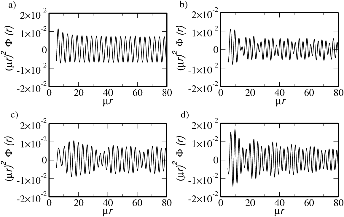
Figure 5: Asymptotic screened potential (in units of $Q\mu/\epsilon_{0}$) of doped graphene for various spin-orbit coupling parameters: (a) $(\lambda_{R}/\mu,\lambda_{I}/\mu)=(0,0.3)$, (b) $(0.3,0.15)$, (c) $(0.15,0.3)$, and (d) $(0.3,0.3)$.

III.2 Finite doping

We now continue with the case of a finite chemical potential lying in the conduction band (the $p$-doped case is analogous). The free polarization in the doped case reads

$$\chi_{0}(q,\omega)=\bar{\chi}_{0}(q,\omega)+\delta\chi_{k_{F+}}(q,\omega)+\delta\chi_{k_{F-}}(q,\omega).$$ (13)

$\bar{\chi}_{0}$ is the undoped part given above. The two remaining contributions, $\delta\chi_{k_{F+}}$ and $\delta\chi_{k_{F-}}$, with

$$\delta\chi_{k_{F\pm}}(q,\omega)=\frac{g_{v}}{4\pi^{2}}\sum_{\alpha,\mu,\nu=\pm 1}\mathcal{P}\int_{0}^{k_{F\pm}}d^{2}k\sum_{\alpha=\pm 1}\frac{\alpha\left|\left\langle\chi_{\pm+}(\boldsymbol{k})\Big{|}\chi_{\mu\nu}(\boldsymbol{k}+\boldsymbol{q})\right\rangle\right|^{2}}{\omega+i0-\alpha\left[E_{\mu\nu}(\boldsymbol{k}+\boldsymbol{q})-E_{\pm+}(\boldsymbol{k})\right]}$$ (14)

refer to transitions with initial states in band $E_{++}$ and $E_{-+}$, respectively. As the expressions for the extrinsic real and imaginary part of the free polarization function are quite lengthy, we refer to Appendix B where the results including major steps of the derivation can be found.

Similar to the undoped case, the density correlation function of graphene is finite at $\omega=q$ for $\lambda_{R}\neq\lambda_{I}$ and divergent for $\lambda_{R}=\lambda_{I}$. However, this divergence vanishes in the RPA improved result.Wunsch

From the shape of the Fermi surface and the dispersion relation as given in Eq. (3), we can determine the boundaries of the dissipative electron-hole continuum.Guil In Fig. 2 this is shown for the particular choice of $\lambda_{R}=2\lambda_{I}=0.3\mu$. In general, the lower and upper boundaries of the damped region I are given by

$$\omega_{low}^{I}=\text{max}\left\{0,\;\sqrt{\left(k_{F-}-q\right)^{2}+\lambda_{+}^{2}}-\sqrt{k_{F-}^{2}+\lambda_{+}^{2}}\right\}$$

and

$$\omega_{up}^{I}=\text{max} \left\{\sqrt{\left(k_{F-}+q\right)^{2}+\lambda_{+}^{2}}-\sqrt{k_{F-}^{2}+\lambda_{+}^{2}},\right.$$

$$\left.\sqrt{\left(k_{F+}+q\right)^{2}+\lambda_{-}^{2}}-\sqrt{k_{F+}^{2}+\lambda_{-}^{2}}\right\},$$

respectively. Region I is due to intraband transitions from band $E_{\pm+}(\boldsymbol{k})$ to $E_{\pm+}(\boldsymbol{k}+\boldsymbol{q})$. Region II accounts for interband transitions between conduction bands and is confined by

$$\omega_{up/low}^{II}=\sqrt{\left(k_{F-}\pm q\right)^{2}+\lambda_{-}^{2}}-\sqrt{k_{F-}^{2}+\lambda_{+}^{2}}+2\lambda_{R}.$$

For region III the lower limit reads

$$\omega_{low}^{III}=\text{min} \left\{\sqrt{\left(k_{F-}-q\right)^{2}+\lambda_{+}^{2}}+\sqrt{k_{F-}^{2}+\lambda_{-}^{2}}-2\lambda_{R},\right.$$

$$\left.\sqrt{\left(k_{F+}-q\right)^{2}+\lambda_{-}^{2}}+\sqrt{k_{F+}^{2}+\lambda_{-}^{2}}\right\}$$

while there is no restriction to the upper boundary. This part is due to transitions between valence and conduction bands.

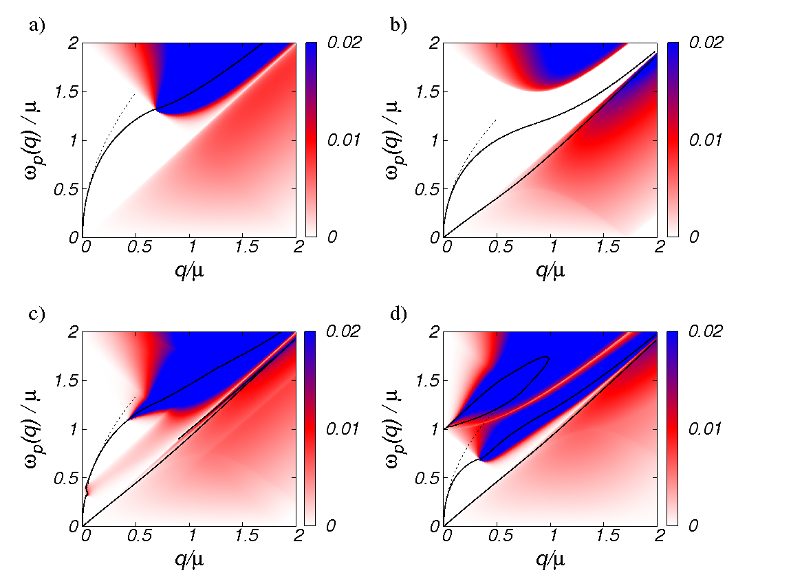
Figure 6: Density plot of $\operatorname{Im}\left\{-1/\varepsilon(q,\omega)\right\}$ for various spin-obit coupling parameters: (a) $(\lambda_{R}/\mu,\lambda_{I}/\mu)=(0,0)$, (b) $(0,0.5)$, (c) $(0.25,0.25)$, (d) $(0.5,0)$. Straight lines correspond to the numerically calculated zeros of the real part of the dielectric function while dashed lines represent the long-wavelength result of Eq. (19).

IV Screening of impurities

The potential of a screened charged impurity is obtained from the definition of the dielectric function,

$$\Phi(r)=\frac{Q}{\epsilon_{0}}\int_{0}^{\infty}dq\;\frac{J_{0}(qr)}{\varepsilon(q,0)}.$$ (15)

$J_{0}(x)$ is the Bessel function of the first kind and $Q$ the charge of the impurity. Making use of Eq. (15) the screened potential for the undoped system is calculated numerically where $\Phi(r)$ is mainly determined by the long-wavelength behavior of the static correlator.Gamayun_2011 As can be seen from Fig. 3(a), the long-wavelength limit of the polarization $\bar{\chi}_{0}(0,0)$ is finite in the semimetallic state ($\lambda_{R}>\lambda_{I}$) and zero otherwise while for large momenta all functions scale like $1/q$. From Fig. 4(a) we can see that for $\lambda_{I}\gtrsim\lambda_{R}$ the potential scales like $\Phi(r)\propto 1/r$ at large distances. For $\lambda_{R}>\lambda_{I}$ the asymptotic potential behaves as $\Phi(r)\propto 1/r^{3}$; see Fig. 4(b). The actual values of $\mu r$ at which the above asymptotics are appropriate approximations depend on the difference of $\lambda_{R}$ and $\lambda_{I}$. As mentioned in the introduction, the two different parameter regimes belong to different phases separated by the quantum critical point at $\lambda_{R}=\lambda_{I}$.

The static density correlator for the doped system is much more complicated. Integrals of the form (15) are usually treated analytically by approximating the Bessel function by its asymptotic values. The subsequent Fourier integral can then be solved with the Lighthill theorem.Lighthill The above theorem states that singularities in the derivatives of the dielectric function give rise to a characteristic, algebraic, oscillating decay of the screened potential. Physically, these Friedel oscillations are due to backscattering on the Fermi surface. We can thus make qualitative predictions for the potential $\Phi(r)$ at large distances away from the impurity, only from the analytical structure of the polarization function without carrying out the integration. Afterwards these predictions are compared to the exact numerical solution.

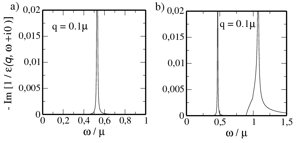
Figure 7: Energy loss function $\operatorname{Im}\left\{-1/\varepsilon(q,\omega+i0)\right\}$ for fixed $q=0.1\mu$ with (a) $\lambda_{R}=0$, $\lambda_{I}=0.5\mu$ and (b) $\lambda_{R}=0.5\mu$, $\lambda_{I}=0$.

For non zero SOC and $\lambda_{R}\neq\lambda_{I}$ the first derivative of the polarization function is singular at special points $q=2k_{F\pm}$; see Figs. 3(c) and (d). According to the Lighthill theorem the potential will exhibit a superposition of two different kinds of oscillations whereat $\Phi(r)\propto 1/r^{2}$. This beating should be observable in sufficiently clean samples if the Rashba parameter, and the consequential breaking of the spin-degeneracy, is large enough. For predominant intrinsic SOI, the two oscillatory parts interfere constructively finally yielding an additional spin-degeneracy factor of $g_{s}=2$.Pyat For $\lambda_{R}=\lambda_{I}$ already the first derivative of $\chi_{0}(q,0)$ is singular at $q=2k_{F-}$ while at $q=2k_{F+}$ only the second derivative diverges; see Fig. 3(b). The main contribution in the potential again will be of order $1/r^{2}$. The numerical inspection of $\Phi(r)$ as displayed in Fig. 5 confirms the above predictions.

The resulting potential deviates significantly from the

$$\Phi(r)\propto\frac{\cos{\left(2k_{F}r\right)}}{\left(2k_{F}r\right)^{3}}$$ (16)

behavior of standard graphene within the Dirac cone approximation.Wunsch ; Ando_2006

Nevertheless, including the full dispersion of graphene can also lead to a different decay behavior, i.e., to anisotropic regular Friedel oscillations decaying like $1/r^{2}$.Santos_2011

V Plasmons

Plasmons are defined as the zeros of the dielectric function,

$$\varepsilon(q,\omega_{p}-i\gamma)=0.$$ (17)

For small damping constant $\gamma$, Eq. (17) can be substituted by the approximate equationGuil

$$\operatorname{Re}\left\{\varepsilon(q,\omega_{p})\right\}=0.$$ (18)

Only if $\gamma$ is small compared to $\omega_{p}$, one can speak of collective density fluctuations. For large Landau-damping, it is thus important to also discuss the more general energy loss function $\operatorname{Im}\left\{-1/\varepsilon(q,\omega)\right\}$ which gives the spectral density of the internal excitations of the system.

Similar to Refs. Pyat ; Gamayun_2011 , there are several solutions of Eq. (18) for non zero SOC parameters. In Fig. 6, these solutions are shown as straight lines together with a density plot of the energy loss function $\operatorname{Im}\left\{-1/\varepsilon(q,\omega)\right\}$. One of these solutions has an almost linear dispersion with a sound velocity close to the Fermi velocity which exhibits an ending point for $\lambda_{R}\sim\lambda_{I}$ associated with a double zero of the real part of the dielectric function. However, as can be seen from Figs. 7(a) and (b), this solution does not yield to a resonance in the loss function and does thus not resemble a plasmonic mode. In the case where the gap in the spectrum is closed ($\lambda_{R}>\lambda_{I}$), two additional zeros appear leading to potential high energy modes similar to bilayer graphene.Gamayun_2011 ; Yuan_2011 However, these potential collective modes are damped by interband transitions; i.e., the corresponding peaks in the loss function are broadened out as can be seen from Fig. 7(b) and no clear signature is seen in the density plot.

We are thus left with the branch which is also present for “clean” graphene and which resembles the only genuine plasmonic mode; see Fig. 6(a). Its dispersion $\omega_{p}$ can be approximated in the long-wavelength limit ($q\ll\omega$) bySensarma_2010

$$\omega_{p}^{0}(q)=\beta\sqrt{q},$$ (19)

where the prefactor is given by $\beta=\sqrt{\frac{g_{v}e^{2}}{8\pi\epsilon_{0}}\sum_{\mu=\pm 1}\frac{k_{F\mu}^{2}}{\sqrt{k_{F\mu}^{2}+\lambda_{-\mu}^{2}}}}$. We thus recover the typical $\sqrt{q}$-dispersion of 2D-plasmons.

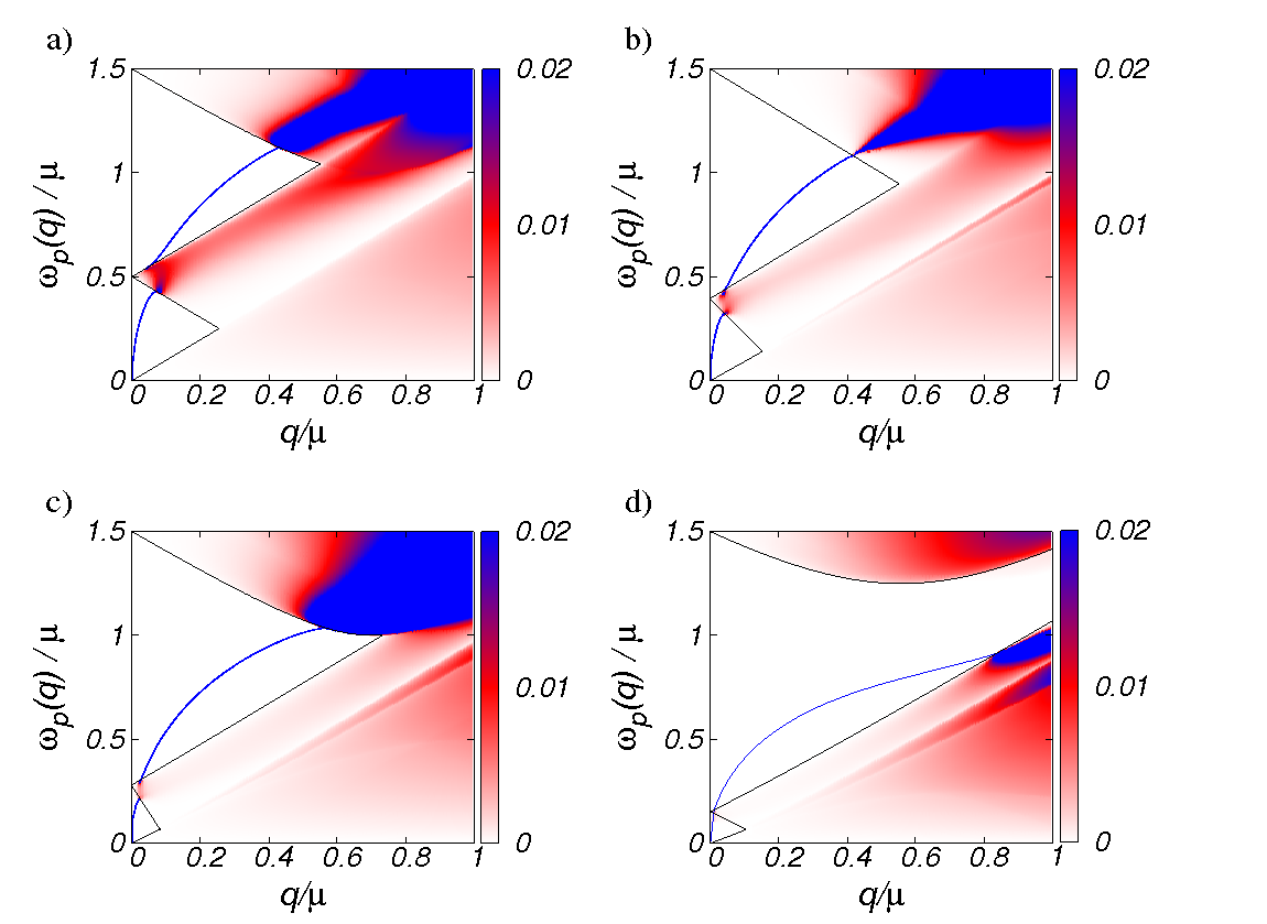
Figure 8: Energy loss function $\operatorname{Im}\left\{-1/\varepsilon(q,\omega+i0)\right\}$ for (a) $(\lambda_{R}/\mu,\lambda_{I}/\mu)=(0.25,0)$, (b) $(0.25,0.25)$, (c) $(0.25,0.5)$, and (d) $(0.25,0.75)$. The straight blue lines show the undamped plasmon modes. The black lines indicate the boundaries of the single-particle continuum (see Sec. III B).

The long-wavelength approximation is shown as a dashed line in Fig. 6 and coincides with the numerical solution, $\omega_{p}$, for small momenta, whereas for larger momenta, the $\omega_{p}$ is red shifted compared to $\omega_{p}^{0}$. If $\lambda_{I}$ is large enough, $\omega_{p}$ remains in the region where Landau damping is absent, see Fig. 6(b),Pyat otherwise it eventually enters the Landau-damped region due to interband transitions from the valence to the conduction band, see Figs. 6(a), (d).

For two occupied conduction bands, which is the case in Fig. 6(c) and in Fig. 8, the plasmon mode is disrupted at $q\approx 0.05\mu$ by a region with a finite imaginary part where it becomes damped. This additional Landau-damped region is due to interband transitions from the two conduction bands. The analytical description of the boundaries of this region can be found in Sec. III B.

This “pseudo gap” of the plasmon dispersion can also be obtained from only considering Eq. (18) since the “plasmon” velocity formally diverges at the entering and exit point as can be seen from Fig. 6(c). The crossing points can alternatively be approximated by looking at the intersection of this region with the analytical long-wavelength approximation of the analytic plasmon dispersion. For the quantum critical point ($\lambda_{R}=\lambda_{I}$), this leads to the critical wave vector

$$q_{cr}^{\pm}=\frac{\left(\beta-\sqrt{\beta^{2}\mp 4\left(k_{F-}-\sqrt{k_{F-}^{2}+4\lambda_{R}^{2}}+2\lambda_{R}\right)}\right)^{2}}{4}\,,$$

and in particular to $q^{-}_{cr}\approx 0.019\mu$ and $q^{+}_{cr}\approx 0.025\mu$ for $\lambda_{R/I}=0.25\mu$. For a proper analysis, the full energy loss function thus needs to be discussed which is done in Fig. 9. It shows how the spectral weight is eventually transferred from the lower to the upper band as momentum is increased, explaining the step in the plasmon spectrum as shown in Fig. 8.

The pseudo gap of the plasmonic mode always appears for $\lambda_{R}<0.5\mu$, since then two conduction bands are occupied independently of the value of $\lambda_{I}$, but it decreases for increasing $\lambda_{I}$ as the dissipative region due to interband transitions diminishes. In the opposite case of $\lambda_{R}>0.5\mu$, either one or two bands can be occupied. For zero intrinsic coupling, the pseudo-gap is absent but increases up to a maximum value at around $\lambda_{I}\approx\lambda_{R}$ for increasing $\lambda_{I}$.

Let us close with a comment on plasmons in undoped graphene. For neutral monolayer graphene and at zero temperature, plasmons can exist if one takes into account a circularly polarized light fieldBusl_2011 or effects beyond RPA,Mishchenko_2008 and in bilayer by including trigonal warping.Wang_2007 In our system, the real part of the dielectric function is always nonzero for the undoped case and thus no plasmons exist.

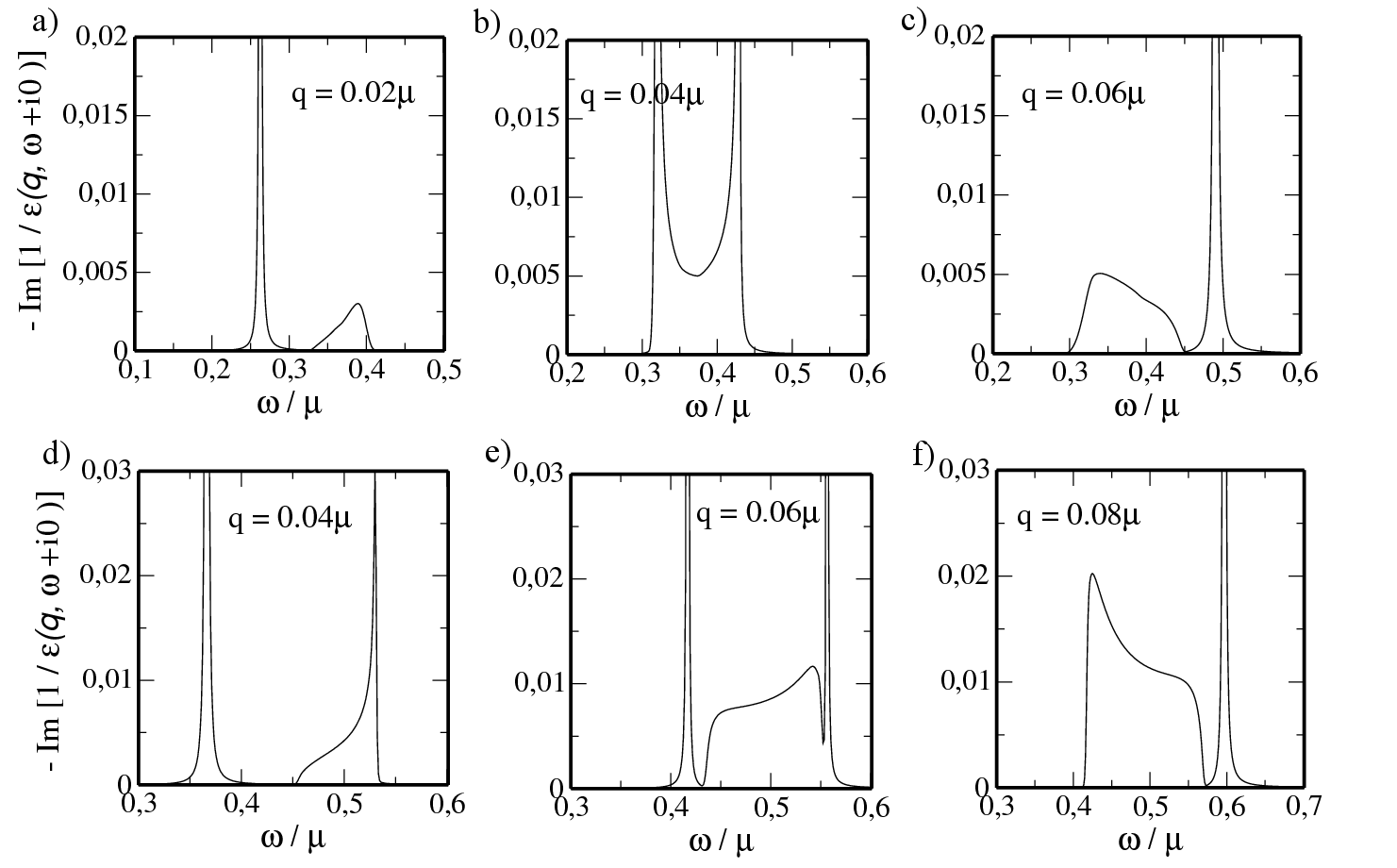
Figure 9: Top: Energy loss function $\operatorname{Im}\left\{-1/\varepsilon(q,\omega+i0)\right\}$ for $\lambda_{R}=0.25\mu=\lambda_{I}=0.25\mu$ and various wave vectors q. Bottom: The same for $\lambda_{R}=0.25\mu$ and $\lambda_{I}=0$.

VI Conclusions and outlook

We have presented analytical and numerical results for the dielectric function of monolayer graphene in the presence of Rashba and intrinsic spin-orbit interactions within the random phase approximation for finite frequency, wave vector, and doping. The cases of predominant Rashba and intrinsic coupling and the case of equally large SOC were opposed.

In the static limit the screening properties due to external impurities were studied. Our findings show that the power-law dependence of the screened potential in the undoped system depends on the ratio of the Rashba and intrinsic parameters. While for $\lambda_{R}>\lambda_{I}$ the screened potential scales like $\Phi(r)\propto 1/r^{3}$, for $\lambda_{I}\geq\lambda_{R}$ a weaker screening, $\Phi(r)\propto 1/r$, was found. For finite Rashba coupling, a beating of Friedel oscillations in the doped system occurs due to the existence of two distinct kinds of Fermi wave vectors. For large $\lambda_{I}\gg\lambda_{R}$, this beating vanishes and the two contributions interfere constructively.

In the last section the influence of SOI on the collective charge excitations was discussed. We found that while only one plasmon mode exists for standard graphene, several new potential modes occur for finite SOC. However, most of these modes are overdamped and can hardly be detected as they lie in the region with finite Landau damping. In the case when the two conduction bands are filled, the undamped plasmon mode is disrupted by a narrow dissipative region strip due to particle-hole excitations. This “pseudo gap” might be useful to gain further control in possible plasmonic circuitries based on graphene.

As already mentioned in the beginning, our findings go even beyond monolayer graphene. For purely Rashba coupling the dielectric function presented in this work equals that of bilayer graphene. The role of the SOC parameter is then played by the interlayer hopping amplitude $t_{IL}$ being several orders of magnitude larger than $\lambda_{R}$. Additionally, the Hamiltonian in Eq. (1) generally describes a system known as the Kane-Mele topological insulator.Kane_2005 Our discussion can thus be fully adopted to materials modeled by this Hamiltonian. Besides that, our findings might also be relevant for other monolayers with similar symmetry properties compared to those of graphene, e.g. MoS₂, where SOC is naturally strong.Xiao_2012 A detailed study of the dielectric properties of MoS₂, however, is left open for future works.

Appendix A Details of the calculation of the undoped polarization

The undoped polarization is composed of four parts,

$$\bar{\chi}_{0}(q,\omega)=\sum_{\eta_{i}=\pm}\chi^{\eta_{1}-\to\eta_{3}+}(q,\omega).$$ (20)

As two of them can be obtained by a simple substitution, i.e., $\chi^{--\to++}_{\lambda_{R}}(q,\omega)=\chi^{+-\to-+}_{-\lambda_{R}}(q,\omega)$ and $\chi^{+-\to++}_{\lambda_{R}}(q,\omega)=\chi^{--\to-+}_{-\lambda_{R}}(q,\omega)$ only two contributions remain. With the help of the Dirac identity the imaginary parts read

$$\operatorname{Im}\left\{\chi^{--\to-+}(q,\omega)\right\}=-\frac{g_{v}}{4\pi}\int d^{2}k\sum_{\alpha=\pm 1}\alpha\left|\left\langle\chi_{--}(\boldsymbol{k})\Big{|}\chi_{-+}(\boldsymbol{k}+\boldsymbol{q})\right\rangle\right|^{2}\delta\left[\omega-\alpha\left(E_{-+}(\boldsymbol{k}+\boldsymbol{q})-E_{--}(\boldsymbol{k})\right)\right]$$ (21)

$$=\frac{g_{v}}{16}\;\theta\left[\omega^{2}-q^{2}-4{\lambda_{+}}^{2}\right]\left[\frac{3q^{4}-4{\lambda_{+}}^{2}q^{2}-5q^{2}\omega^{2}+2\omega^{4}}{\left(\omega^{2}-q^{2}\right)^{3/2}}-\frac{\left|q^{2}-\omega\left(\omega-2\lambda_{+}\right)\right|+\left|q^{2}-\omega\left(\omega+2\lambda_{+}\right)\right|}{\omega}\right]$$ (22)

and

$$\operatorname{Im}\left\{\chi^{+-\to-+}(q,\omega)\right\}=-\frac{g_{v}}{4\pi}\int d^{2}k\sum_{\alpha=\pm 1}\alpha\left|\left\langle\chi_{+-}(\boldsymbol{k})\Big{|}\chi_{-+}(\boldsymbol{k}+\boldsymbol{q})\right\rangle\right|^{2}\delta\left[\omega-\alpha\left(E_{-+}(\boldsymbol{k}+\boldsymbol{q})-E_{+-}(\boldsymbol{k})\right)\right]$$ (23)

$$=-\frac{g_{v}}{8\pi}\int_{\left|\lambda_{-}\right|}^{\infty}dy\frac{\sqrt{\omega_{+}^{2}-q^{2}}\sqrt{\frac{q^{2}}{4}\frac{\left(q^{2}-\omega_{+}^{2}+4\lambda_{I}^{2}\right)\left(q^{2}-\omega_{+}^{2}+4\lambda_{R}^{2}\right)}{\left(q^{2}-\omega_{+}^{2}\right)^{2}}-\left[y-\frac{\omega_{+}}{2}\left(1+\frac{4\lambda_{R}\lambda_{I}}{q^{2}-\omega_{+}^{2}}\right)\right]^{2}}}{(y-\lambda_{-})(\omega-y+\lambda_{-})}$$

$$\hskip 56.9055pt\times\theta\left[1-\left(\frac{\omega_{+}^{2}-q^{2}-2\omega_{+}y-4\lambda_{R}\lambda_{I}}{2q\sqrt{y^{2}-\lambda_{-}^{2}}}\right)^{2}\right]\theta\left[\omega_{+}^{2}-q^{2}-4\gamma^{2}\right]$$ (24)

$$=-\frac{g_{v}}{8}\,\theta\left[\omega_{\pm}^{2}-q^{2}-4\gamma^{2}\right]\left[\sqrt{\omega_{\pm}^{2}-q^{2}}-\frac{\left|q^{2}-\omega\left(\omega\pm 2\lambda_{-}\right)\right|}{2\omega}-\frac{\left|q^{2}-\omega\left(\omega\pm 2\lambda_{+}\right)\right|}{2\omega}\,\right]$$ (25)

with $\gamma=\text{max}\left\{\lambda_{R},\lambda_{I}\right\}$ and $y=\sqrt{k^{2}+\lambda_{-}^{2}}$.

We can now make use of Eq. (9) in order to find the real part. The first contribution reads

$$\operatorname{Re}\left\{\chi^{--\to-+}(q,\omega)\right\}=\frac{2}{\pi}\mathcal{P}\int_{0}^{\infty}d\omega^{\prime}\frac{\omega^{\prime}}{\omega^{\prime 2}-\omega^{2}}\operatorname{Im}\left\{\chi^{--\to-+}(q,\omega^{\prime})\right\}$$ (26)

$$=\frac{g_{v}}{8\pi}\left\{-K_{\lambda}(4\lambda^{2})+\mathcal{L}_{\lambda}(\sqrt{q^{2}+4\lambda^{2}})+2\mathcal{L}_{-\lambda}(\sqrt{q^{2}+\lambda^{2}}+\lambda)-\mathcal{L}_{-\lambda}(\sqrt{q^{2}+4\lambda^{2}})\right.$$

$$\left.\hskip 56.9055pt+\theta\left[q-\omega\right]\frac{3q^{2}\omega^{2}+4q^{2}\lambda^{2}-3q^{4}-2\omega^{4}}{(q^{2}-\omega^{2})^{3/2}}\frac{\pi}{2}\right\}$$ (27)

Here we introduced the functions

$$K_{\lambda}(x)=2\sqrt{x}+\frac{4q^{2}\lambda^{2}}{(q^{2}-\omega^{2})\sqrt{x}}-\left(3q^{4}-5q^{2}\omega^{2}+2\omega^{4}-4q^{2}\lambda^{2}\right)\operatorname{Re}\left\{\frac{\operatorname{arctan}\left(\frac{\sqrt{x}}{\sqrt{q^{2}-\omega^{2}}}\right)}{(q^{2}-\omega^{2})^{3/2}}\right\}$$ (28)

and

$$\mathcal{L}_{\lambda}(x)=x+\lambda\ln{\left|x^{2}-\omega^{2}\right|}-\frac{\omega^{2}-q^{2}}{2\omega}\ln{\left|\frac{x+\omega}{x-\omega}\right|}.$$ (29)

The second contribution can be solved in a similar way,

$$\operatorname{Re}\left\{\chi^{+-\to-+}(q,\omega)\right\}=\frac{2}{\pi}\mathcal{P}\int_{0}^{\infty}d\omega^{\prime}\frac{\omega^{\prime}}{\omega^{\prime 2}-\omega^{2}}\operatorname{Im}\left\{\chi^{+-\to-+}(q,\omega^{\prime})\right\}$$

$$=-\frac{g_{v}}{4\pi}\left[2\lambda_{R}(1+\ln 4)-\frac{1}{2}\operatorname{Re}\left\{\sqrt{q^{2}-(\omega+2\lambda_{R})^{2}}\arcsin{\frac{\omega+2\lambda_{R}}{q}}-\sqrt{q^{2}-(-\omega+2\lambda_{R})^{2}}\arcsin{\frac{-\omega+2\lambda_{R}}{q}}\right\}\right.$$

$$\left.\hskip 56.9055pt-\frac{1}{2}\left[G_{\frac{\omega}{2}+\lambda_{R}}\left(\sqrt{q^{2}+4\gamma^{2}}-\omega-2\lambda_{R}\right)+G_{-\frac{\omega}{2}+\lambda_{R}}\left(\sqrt{q^{2}+4\gamma^{2}}+\omega-2\lambda_{R}\right)\right]\right.$$

$$\left.\hskip 56.9055pt+\theta\left[\lambda_{R}+\lambda_{I}\right]\mathcal{L}_{\lambda_{-}}\left(\sqrt{q^{2}+\lambda_{-}^{2}}-\lambda_{-}\right)-\frac{1}{2}\operatorname{sign}\left(\lambda_{R}+\lambda_{I}\right)\mathcal{L}_{\lambda_{-}}\left(\sqrt{q^{2}+4\gamma^{2}}-2\lambda_{R}\right)\right.$$

$$\left.\hskip 56.9055pt+\theta\left[\lambda_{R}-\lambda_{I}\right]\mathcal{L}_{\lambda_{+}}\left(\sqrt{q^{2}+\lambda_{+}^{2}}-\lambda_{+}\right)-\frac{1}{2}\operatorname{sign}\left(\lambda_{R}-\lambda_{I}\right)\mathcal{L}_{\lambda_{+}}\left(\sqrt{q^{2}+4\gamma^{2}}-2\lambda_{R}\right)\;\right]$$ (30)

with

$$G_{\omega}(x)= \sqrt{(x+\omega)^{2}-q^{2}}+\omega\ln{(\sqrt{(x+\omega)^{2}-q^{2}}+x+\omega)}$$

$$-\sqrt{\omega^{2}-q^{2}}\ln{\frac{\omega x+\omega^{2}-q^{2}+\sqrt{\omega^{2}-q^{2}}\sqrt{(x+\omega)^{2}-q^{2}}}{x}}$$ (31)

Appendix B Details of the calculation of the doped polarization

The extrinsic part for the band $E_{-+}$,

$$\delta\chi_{k_{F-}}(q,\omega)=\frac{g_{v}}{4\pi^{2}}\sum_{\mu,\nu=\pm 1}\mathcal{P}\int_{0}^{k_{F-}}d^{2}k\sum_{\alpha=\pm 1}\frac{\alpha\left|\left\langle\chi_{-+}(\boldsymbol{k})\Big{|}\chi_{\mu\nu}(\boldsymbol{k}+\boldsymbol{q})\right\rangle\right|^{2}}{\omega+i0-\alpha\left[E_{\mu\nu}(\boldsymbol{k}+\boldsymbol{q})-E_{-+}(\boldsymbol{k})\right]},$$ (32)

can be summarized as

$$\delta\chi_{k_{F-}}(q,\omega)= \frac{g_{v}}{4\pi^{2}}\mathcal{P}\int_{0}^{k_{F-}}d^{2}k\left[\frac{\left(\omega+i0+\sqrt{k^{2}+\lambda_{+}^{2}}+\sqrt{\left|\boldsymbol{k}+\boldsymbol{q}\right|^{2}+\lambda_{+}^{2}}\right)\left|\left\langle\chi_{-+}(\boldsymbol{k})\Big{|}\chi_{--}(\boldsymbol{k}+\boldsymbol{q})\right\rangle\right|^{2}}{\left(\omega+i0+\sqrt{k^{2}+\lambda_{+}^{2}}\right)^{2}-\left(\left|\boldsymbol{k}+\boldsymbol{q}\right|^{2}+\lambda_{+}^{2}\right)}\right.$$

$$\left.+\frac{\left(\omega+i0+\sqrt{k^{2}+\lambda_{+}^{2}}-\sqrt{\left|\boldsymbol{k}+\boldsymbol{q}\right|^{2}+\lambda_{+}^{2}}\right)\left|\left\langle\chi_{-+}(\boldsymbol{k})\Big{|}\chi_{--}(\boldsymbol{k}+\boldsymbol{q})\right\rangle\right|^{2}}{\left(\omega+i0+\sqrt{k^{2}+\lambda_{+}^{2}}\right)^{2}-\left(\left|\boldsymbol{k}+\boldsymbol{q}\right|^{2}+\lambda_{+}^{2}\right)}\right.$$

$$\left.+\frac{\left(\omega_{-}+i0+\sqrt{k^{2}+\lambda_{+}^{2}}-\sqrt{\left|\boldsymbol{k}+\boldsymbol{q}\right|^{2}+\lambda_{-}^{2}}\right)\left|\left\langle\chi_{-+}(\boldsymbol{k})\Big{|}\chi_{+-}(\boldsymbol{k}+\boldsymbol{q})\right\rangle\right|^{2}}{\left(\omega_{-}+i0+\sqrt{k^{2}+\lambda_{+}^{2}}\right)^{2}-\left(\left|\boldsymbol{k}+\boldsymbol{q}\right|^{2}+\lambda_{-}^{2}\right)}\right.$$

$$\left.+\frac{\left(\omega_{-}+i0+\sqrt{k^{2}+\lambda_{+}^{2}}+\sqrt{\left|\boldsymbol{k}+\boldsymbol{q}\right|^{2}+\lambda_{-}^{2}}\right)\left|\left\langle\chi_{-+}(\boldsymbol{k})\Big{|}\chi_{++}(\boldsymbol{k}+\boldsymbol{q})\right\rangle\right|^{2}}{\left(\omega_{-}+i0+\sqrt{k^{2}+\lambda_{+}^{2}}\right)^{2}-\left(\left|\boldsymbol{k}+\boldsymbol{q}\right|^{2}+\lambda_{-}^{2}\right)}\right.$$

$$\left.+\left(\omega\to-\omega\right)\right.\Big{]}$$ (33)

where ($\omega\to-\omega$), and thus $(\omega_{-}\to-\omega_{+}$), denotes terms with the sign of the frequency changed compared to the preceding expression. The corresponding expression for $E_{++}$ can be obtained by substituting $\lambda_{R}\to-\lambda_{R}$ and $k_{F-}\to k_{F+}$. After carrying out the angle integration for the real part and choosing a proper substitution, $x=\sqrt{k^{2}+\lambda_{+}^{2}}-\lambda_{+}$, we arrive at

$$\operatorname{Re}\left\{\delta\chi_{k_{F-}}(q,\omega)\right\}=-\frac{g_{v}}{2\pi}\operatorname{Re}\left\{\mathcal{P}\int_{\epsilon}^{\mu-\lambda_{I}}dx\left[\frac{x+\lambda_{R}}{2x}\right.\right.$$

$$\left.\left.+\frac{\left[q^{2}-(x+\frac{\omega}{2})(x+\frac{\omega}{2}+\lambda_{+})\right]^{2}}{x(x+\frac{\omega}{2})}\frac{\operatorname{sign}\left(q^{2}-\omega^{2}-2\omega(x+\lambda_{+})\right)}{\sqrt{q^{2}-\omega^{2}}\sqrt{\frac{q^{2}}{4}\left(1+\frac{4\lambda_{+}^{2}}{q^{2}-\omega^{2}}\right)-(x+\frac{\omega}{2}+\lambda_{+})^{2}}}\right.\right.$$

$$\left.\left.-\frac{\sqrt{q^{2}-\omega_{-}^{2}}\;\sqrt{\frac{q^{2}}{4}\frac{\left(q^{2}-\omega_{+}^{2}+4\lambda_{I}^{2}\right)\left(q^{2}-\omega_{+}^{2}+4\lambda_{R}^{2}\right)}{\left(q^{2}-\omega_{+}^{2}\right)^{2}}-(x+\frac{\omega_{+}}{2}\left(1+\frac{4\lambda_{R}\lambda_{I}}{q^{2}-\omega_{+}^{2}}\right)+\lambda_{+})^{2}}}{4x(x+\omega)}\times\right.\right.$$

$$\left.\left.\hskip 28.45274pt\times\operatorname{sign}\left(q^{2}-\omega_{-}^{2}-2\omega_{-}(x+\lambda+)-4\lambda_{R}\lambda_{I}\right)\right]\quad+\quad\left(\omega\to-\omega\right)\;\right.\Big{\}}$$ (34)

These integrals can now be solved in terms of trigonometric and hyperbolic functions.Gradshteyn In order to simplify the expressions we use the shorthand notation Gamayun_2011

$$\hat{f}(x)\Big{|}_{a}^{b}=\operatorname{sign}\left(b-x\right)\left(f(b)-f(x)\right)-\operatorname{sign}\left(a-x\right)\left(f(a)-f(x)\right)$$ (35)

The result can then be written as

$$\operatorname{Re}\left\{\delta\chi_{k_{F-}}(q,\omega)\right\}=-\frac{g_{v}\left(\mu-\lambda_{I}\right)}{2\pi}-\frac{g_{v}\lambda_{R}}{4\pi}\ln{\frac{\mu-\lambda_{I}}{\epsilon}}$$

$$+\frac{g_{v}}{2\pi\omega}\operatorname{Re}\left\{\operatorname{sign}\left(\omega\right)\left(\hat{\mathcal{R}}_{1}^{\omega}\left(\frac{q^{2}-\omega^{2}-2\omega\lambda_{+}}{2\omega}\right)\Big{|}_{\epsilon}^{\mu-\lambda_{I}}-\hat{\mathcal{R}}_{1}^{-\omega}\left(\frac{q^{2}+\omega^{2}-2\omega\lambda_{+}}{2\omega}\right)\Big{|}_{\omega}^{\mu-\lambda_{I}+\omega}\right)\right.$$

$$\left.-\operatorname{sign}\left(\omega_{-}\right)\left(\hat{\mathcal{R}}_{2}^{\omega}\left(\frac{q^{2}-\omega^{2}+2\lambda_{-}\omega}{2\omega_{-}}\right)\Big{|}_{\epsilon}^{\mu-\lambda_{I}}-\hat{\mathcal{R}}_{2}^{-\omega}\left(\frac{q^{2}+\omega^{2}-2\lambda_{+}\omega}{2\omega_{-}}\right)\Big{|}_{\omega}^{\mu-\lambda_{I}+\omega}\right)\right\}\quad+\quad\left(\omega\to-\omega\right)$$ (36)

with

$$\mathcal{R}_{i}^{\omega}(x)=\frac{c_{i}^{\omega}}{\gamma_{i}^{\omega}}\sqrt{r_{i}^{\omega}}-\frac{\sqrt{\alpha_{i}^{\omega}}}{4}\ln{\frac{2\alpha_{i}^{\omega}+\beta_{i}^{\omega}x+2\sqrt{\alpha_{i}^{\omega}}\sqrt{r_{i}^{\omega}}}{x}}+\frac{\tilde{c}_{i}^{\omega}}{\sqrt{\gamma_{i}^{\omega}}}\ln{\left(2\sqrt{\gamma_{i}^{\omega}}\sqrt{r_{i}^{\omega}}+2\gamma_{i}^{\omega}x+\beta_{i}^{\omega}\right)}$$ (37)

and $r_{i}^{\omega}=\alpha_{i}^{\omega}+\beta_{i}^{\omega}x+\gamma_{i}^{\omega}x^{2}$. The coefficients read

$$\alpha_{1}^{\omega} =\frac{\left(q^{2}-\omega\left(\omega+2\lambda_{+}\right)\right)^{2}}{4}\quad,\quad\alpha_{2}^{\omega}=\frac{\left(q^{2}-\omega\left(\omega_{-}-2\operatorname{sign}\left(\omega\right)\lambda_{I}\right)\right)^{2}}{4}$$

$$\beta_{1}^{\omega}=\left(\omega^{2}-q^{2}\right)\left(2\lambda_{+}+\omega\right)\quad,\quad\beta_{2}^{\omega}=8\lambda_{R}^{2}\lambda_{I}-2\lambda_{R}\lambda_{I}\left(\omega+\left|\omega\right|\right)-\operatorname{sign}\left(\omega\right)\left(\omega-2\lambda_{R}\right)\left(q^{2}-\omega_{-}^{2}\right)$$

$$\gamma_{1}^{\omega} =\omega^{2}-q^{2}\quad,\quad\gamma_{2}^{\omega}=\left|\omega\right|_{-}^{2}-q^{2}\quad,\quad c_{1}^{\omega}=\frac{x^{2}}{3}+\frac{2\lambda_{+}+7\omega}{12}x+\frac{4\lambda_{+}^{2}-4q^{2}+8\lambda_{+}^{2}+5\omega^{2}}{8}-\frac{2\alpha_{1}^{\omega}}{3\gamma_{1}^{\omega}}$$

$$\tilde{c}_{1}^{\omega} =\frac{\alpha_{1}^{\omega}\left(2\lambda_{+}-\omega\right)}{4\gamma_{1}^{\omega}}+\frac{3\omega^{3}+6\lambda_{+}^{2}\omega^{2}-4(q^{2}+\lambda_{+}^{2})\omega-8\lambda_{+}^{3}}{16}\quad,\quad c_{2}^{\omega}=\frac{\gamma_{2}^{\omega}}{4}\quad,\quad\tilde{c}_{2}^{\omega}=\frac{\beta_{2}^{\omega}}{8}$$

The calculation of the imaginary part is quite similar. Starting from Eq. (33) and carrying out the angle integration in a way similar to the real part, we arrive at

$$\operatorname{Im}\left\{\delta\chi_{k_{F-}}(q,\omega)\right\}=\frac{g_{v}}{2\pi}\operatorname{Re}\left\{\mathcal{P}\int_{\epsilon}^{\mu-\lambda_{I}}dx\left[\frac{\left[q^{2}-(x+\frac{\omega}{2})(x+\frac{\omega}{2}+\lambda_{+})\right]^{2}}{x(x+\frac{\omega}{2})}\frac{\operatorname{sign}\left(x-\lambda_{-}+\omega\right)}{\sqrt{\omega^{2}-q^{2}}\sqrt{\frac{q^{2}}{4}\left(1+\frac{4\lambda_{+}^{2}}{q^{2}-\omega^{2}}\right)-(x+\frac{\omega}{2}+\lambda_{+})^{2}}}\right.\right.$$

$$\left.\left.-\frac{\sqrt{\omega_{-}^{2}-q^{2}}\sqrt{\frac{q^{2}}{4}\frac{\left(q^{2}-\omega_{+}^{2}+4\lambda_{I}^{2}\right)\left(q^{2}-\omega_{+}^{2}+4\lambda_{R}^{2}\right)}{\left(q^{2}-\omega_{+}^{2}\right)^{2}}-(x+\frac{\omega_{+}}{2}\left(1+\frac{4\lambda_{R}\lambda_{I}}{q^{2}-\omega_{+}^{2}}\right)+\lambda_{+})^{2}}}{4x(x+\omega)}\operatorname{sign}\left(x+\lambda_{+}+\omega\right)\;\right]\quad-\quad\left(\omega\to-\omega\right)\;\right.\Big{\}}$$ (38)

The result can again be written as

$$\operatorname{Im}\left\{\delta\chi_{k_{F-}}(q,\omega)\right\}=\frac{g_{v}}{2\pi\omega}\operatorname{Re}\left\{\frac{1}{i}\hat{\mathcal{R}}_{1}^{\omega}\left(-\lambda_{+}-\omega\right)\Big{|}_{\epsilon}^{\mu-\lambda_{I}}-\frac{1}{i}\hat{\mathcal{R}}_{1}^{\omega}\left(-\lambda_{+}\right)\Big{|}_{\omega}^{\mu-\lambda_{I}+\omega}\right.$$

$$\left.-\frac{1}{i}\theta\left[-\omega\right]\theta\left[\mu-\lambda_{I}+\omega\right]\operatorname{sign}\left(\lambda_{+}\right)\left[R_{1}^{\omega}(-\epsilon)-R_{1}^{\omega}(\epsilon)\right]+i\hat{\mathcal{R}}_{2}^{\omega}\left(\lambda_{-}-\omega\right)\Big{|}_{\epsilon}^{\mu-\lambda_{I}}-i\hat{\mathcal{R}}_{2}^{\omega}\left(\lambda_{-}\right)\Big{|}_{\omega}^{\mu-\lambda_{I}+\omega}\right.$$

$$\left.-i\theta\left[-\omega\right]\theta\left[\mu-\lambda_{I}+\omega\right]\operatorname{sign}\left(-\lambda_{-}\right)\left[R_{2}^{\omega}(-\epsilon)-R_{2}^{\omega}(\epsilon)\right]\right\}\quad-\quad\left(\omega\to-\omega\right)$$ (39)

The limit $\epsilon\to 0$ in Eqs. (36) and (39) can now be taken safely giving finite results.

References

- (1) P. R. Wallace, Phys. Rev. 71, 622 (1947).
- (2) A. H. Castro Neto, F. Guinea, N. M. R. Peres, K. S. Novoselov, and A. K. Geim, Rev. Mod. Phys. 81, 109 (2009).
- (3) C. L. Kane and E. J. Mele, Phys. Rev. Lett. 95, 226801 (2005).
- (4) M. Pletyuhkov and V. Gritsev, Phys. Rev. B 74, 045307 (2006).
- (5) S. M. Badalyan, A. Matos-Abiague, G. Vignale, and J. Fabian, Phys. Rev. B 79, 205305 (2009); 81, 205314 (2010).
- (6) C. A. Ullrich and M. E. Flatte, Phys. Rev. B 68, 235310 (2003).
- (7) J. Schliemann, Phys. Rev. B 74, 045214 (2006); 84, 155201 (2011); Europhys. Lett. 91, 67004 (2010).
- (8) B. Wunsch, T. Stauber, F. Sols, and F. Guinea, New J. Phys. 8, 316 (2006).
- (9) E. H. Hwang and S. Das Sarma, Phys. Rev. B 75, 205418 (2007).
- (10) A. Principi, M. Polini, and G. Vignale, Phys. Rev. B 80, 075418 (2009).
- (11) T. Stauber, J. Schliemann, and N. M. R. Peres, Phys. Rev. B 81, 085409 (2010).
- (12) T. Stauber and G. Gomez-Santos, Phys. Rev. B 82, 155412 (2010).
- (13) T. Stauber, Phys. Rev. B 82, 201404(R) (2010).
- (14) P. K. Pyatkovskiy, J. Phys. Condens. Matter 21, 025506 (2009).
- (15) X.-F. Wang and T. Chakraborty, Phys. Rev. B 75, 033408 (2007).
- (16) A. Scholz and J. Schliemann, Phys. Rev. B 83, 235409 (2011).
- (17) G. Borghi, M. Polini, R. Asgari, and A. H. MacDonald, Phys. Rev. B 80, 241402(R) (2009).
- (18) O. V. Gamayun, Phys. Rev. B 84, 085112 (2011).
- (19) S. Yuan, R. Roldan, and M. I. Katsnelson, Phys. Rev. B 84, 035439 (2011).
- (20) T. Stauber and G. Gómez-Santos, Phys. Rev. B 85, 075410 (2012).
- (21) R. E. V. Profumo, R. Asgari, Marco Polini, and A. H. MacDonald, Phys. Rev. B 85, 085443 (2012).
- (22) C. Triola and E. Rossi, Phys. Rev. B 86, 161408 (2012).
- (23) M. H. Schultz, A. P. Jauho, and T. G. Pedersen, Phys. Rev. B 84, 045428 (2011).
- (24) M. Busl, G. Platero, and A. P. Jauho, Phys. Rev. B 85, 155449 (2012).
- (25) K.-H. Ding, G. Zhou, Z.-G. Zhu, and J. Berakdar, J. Phys. Condens. Matter 20, 345228 (2008).
- (26) P. Ingenhoven, J. Z. Bernad, U. Zülicke, and R. Egger, Phys. Rev. B 81, 035421 (2010).
- (27) A. Hill, A. Sinner, K. Ziegler, arXiv:1005.3211v2.
- (28) A. H. Castro Neto and F. Guinea, Phys. Rev. Lett. 103, 026804 (2009).
- (29) C. Weeks, J. Hu, J. Alicea, M. Franz, and R. Wu, Phys. Rev. X 1, 021001 (2011).
- (30) D. Ma, Z. Li, Z. Yang, Carbon 50, 297-305 (2012).
- (31) A. Varykhalov, J. Sánchez-Barriga, A. M. Shikin, C. Biswas, E. Vescovo, A. Rybkin, D. Marchenko, and O. Rader, Phys. Rev. Lett. 101, 157601 (2008).
- (32) Y. S. Dedkov, M. Fonin, U. Rüdiger, and C. Laubschat, Phys. Rev. Lett. 100, 107602 (2008).
- (33) K.-H. Jin and S.-H. Jhi, arXiv:1206.3608v1.
- (34) F. Rana, IEEE Trans. Nanotech. 7, 91 (2008).
- (35) A. Bostwick, F. Speck, T. Seyller, K. Horn, M. Polini, R. Asgari, A. H. MacDonald, and E. Rotenburg, Science 328, 999 (2010).
- (36) M. Gmitra, S. Konschuh, C. Ertler, C. Ambrosch-Draxl, and J. Fabian, Phys. Rev. B 80, 235431 (2009).
- (37) H. Min, B. Sahu, S. K. Banerjee, and A. H. MacDonald, Phys. Rev. B 75, 155115 (2007).
- (38) G. Giuliani and G. Vignale, Quantum Theory of the Electron Liquid (Cambridge University Press, Cambridge, 2005).
- (39) M. J. Lighthill, Introduction to Fourier Analysis and Generalized Functions (Cambridge University Press, Cambridge, 1958)
- (40) T. Ando, J. Phys. Soc. Japan 75, 074716 (2006).
- (41) G. Gómez-Santos and T. Stauber, Phys. Rev. Lett. 106, 045504 (2011).
- (42) R. Sensarma, E. H. Hwang, and S. Das Sarma, Phys. Rev. B 82, 195428 (2010).
- (43) S. Gangadharaiah, A. M. Farid, and E. G. Mishchenko, Phys. Rev. Lett. 100, 166802 (2008).
- (44) X.-F. Wang and T. Chakraborty, Phys. Rev. B 75, 041404(R) (2007).
- (45) I. S. Gradshteyn and I. M. Ryzhik, Table of Integrals, Series, and Products (Academic Press, London, 2000).
- (46) D. Xiao, G. B. Liu, W. Feng, X. Xu, and W. Yao, Phys. Rev. Lett. 108, 196802 (2012).