In-phase and anti-phase synchronization in noisy Hodgkin-Huxley neurons

Abstract

We numerically investigate the influence of intrinsic channel noise on the dynamical response of delay-coupling in neuronal systems. The stochastic dynamics of the spiking is modeled within a stochastic modification of the standard Hodgkin-Huxley model wherein the delay-coupling accounts for the finite propagation time of an action potential along the neuronal axon. We quantify this delay-coupling of the Pyragas-type in terms of the difference between corresponding presynaptic and postsynaptic membrane potentials. For an elementary neuronal network consisting of two coupled neurons we detect characteristic stochastic synchronization patterns which exhibit multiple phase-flip bifurcations: The phase-flip bifurcations occur in form of alternate transitions from an in-phase spiking activity towards an anti-phase spiking activity. Interestingly, these phase-flips remain robust in strong channel noise and in turn cause a striking stabilization of the spiking frequency.

1 Introduction

Time-delayed feedback presents a common mechanism which is found in many biological systems including neuronal systems. Signal transmission time delays in neuronal systems either result from (i) chemical processes in the neuronal synapses where neurotransmitters are released and diffusively overcome the synaptic cleft and/or (ii) from the finite propagation speed of electrical excitations along the neuronal axon. Time delays stemming from chemical synapses are of the order of a few milliseconds, while the axonal conduction delays in both, delay-coupled neurons and autaptic feedback loops, reach values up to tens of milliseconds [1, 2, 3, 4].

As the time scale of the delayed coupling and of the neuronal dynamics become comparable, the delay-coupling gives raise to peculiar synchronization phenomena [5]. In particular, phase synchronization phenomena in neuronal systems are commonly thought to be the basis for many biological relevant processes occurring in the brain [6, 7]. Synchrony of neurons from small brain regions up to large-scale networks of different cortices comes along with transmission time delays. Theoretical and computational studies on neuronal networks with delay-coupling recently highlighted the occurrence of so-called phase-flip bifurcations [8, 9, 10]. The ensemble activity of the coupled neurons change abruptly from in-phase to anti-phase oscillations or vice versa.

With this work we research this objective by considering the influence of internal noise. It is an established fact that noise leads to various prominent effects in neuronal dynamics [11]. Some typical examples that come to mind are stochastic resonance features [12, 13, 14, 15], and noise-assisted synchronization [5, 16, 17, 18]. Within our work the intrinsic noise is due to the stochastic gating of the ion channels, i.e. the so-called channel noise which is inherently coupled to the electrical properties of the axonal cell membrane [19, 20, 21]. Interestingly, it has been shown that intrinsic channel noise does not only lead to the generation of spontaneous action potentials [22], but as well affects the neuronal dynamics at different levels, namely: (i) it can boost the signal quality [14, 15], (ii) enhance the signal transmission reliability [23], (iii) cause frequency- and phase-synchronization features [24, 25, 26, 27, 28] and (iv) may result in a frequency stabilization [29], to name but a few.

The present work is organized as follows: In Sec. 2 we introduce the biophysical model. We review the standard Hodgkin-Huxley model and its generalizations with respect to intrinsic channel noise and a delay-coupling. Numerical methods for simulation are introduced after that. In Sec. 3, the dynamics of a network of two delay-coupled Hodgkin-Huxley neurons is explored both, in the deterministic limit and under consideration of channel noise. As a comparison, we retrospect on the previous work on a single neuron subjected to a delayed feedback loop resulting from autapse in Sec. 4. Our conclusions are given in Sec. 5.

2 Biophysical model setup

We consider a minimal building block of a neuronal network composed of two coupled neurons. As an archetype model for nerve excitation of the individual neuron, we utilize a stochastic generalization of the common Hodgkin-Huxley model. The stochastic generalization accounts for intrinsic membranal conductance fluctuations, i.e. channel noise, being caused by random ion channel gating. Moreover, we account for a delay in the coupling which accounts for a finite propagation time of the action potential along the axon.

2.1 Hodgkin-Huxley-type modelling of two delay-coupled neurons

According to Hodgkin and Huxley, the dynamics of the membrane potential $V_{i}$ with $i=1,2$ of two coupled neuronal cells is given by [30]

$$C\frac{\mathrm{d}}{\mathrm{d}t}V_{i}+G_{\mathrm{K}}(n)\,(V_{i}-V_{\mathrm{K}})$$

$$+G_{\mathrm{Na}}(m,h)\,(V_{i}-V_{\mathrm{Na}})+G_{\mathrm{L}}\,(V_{i}-V_{\mathrm{L}})=I_{i}(t)\,.$$ (1)

Here, $V_{i}$ denotes the membrane potential of the $i$-th cell. The stimulus $I_{i}(t)$ acting on the $i$-th neuron reads:

$$I_{i}(t)=I_{i\mathrm{,ext}}(t)+I_{i,j}^{\tau}(t)\,,\quad i,j=1,2\,,i\neq j\,,$$ (2)

where the bi-directional delay-coupling of Pyragas-type [31] between the two neurons is assumed to be linear in the difference of the membrane potentials of a primary, $i$-th neuron at time $t$ and a secondary, $j$-th neuron at an earlier time, $t-\tau$. The coupling thus reads:

$$I_{i,j}^{\tau}(t)=\kappa\,\left[V_{j}(t-\tau)-V_{i}(t)\right]\,,$$ (3)

where $\kappa$ corresponds to the coupling strength and $\tau$ denotes the finite delay time. The coupling defined in Eq. (3) is of “electrotonic” type, i.e. we consider an idealized situation wherein the coupling is proportional to the difference of presynaptic and postsynaptic membrane potentials. This kind of coupling then corresponds to so-called gap-junctions which allow the bi-directional transport of ions and small molecules from one neuronal cell into another. Unlike the conductance of chemical synapses, the conductance of gap-junctions is independent of the presynaptic and postsynaptic membrane potential and can therefore be modelled by the constant coupling parameter $\kappa$. Possible chemical mechanisms occurring at the synaptic cleft are assumed to be instantaneous as the time scale for signal propagation along the neurons axon is much larger than the corresponding one for the transport process in the synaptic cleft. Note, that the delayed stimulus in Eq. (3) results in an excitatory coupling mechanism in which the spiking of neuron $i$ at an earlier time $t-\tau$ time favors the initiation of a action potential of the other cell at time $t$.

In addition to the delayed, bilinear coupling current we apply a constant current stimulus $I_{i,\mathrm{ext}}$ on the neurons, mimicking the common stimulus of the neuronal environment on the so considered two-neuron network. In absence of the bi-directional coupling the dynamics of each neuron exhibits a bifurcation scenario exhibiting a subcritical Hopf bifurcation. As a consequence, the membranal dynamics displays (i) a stable fix-point, i.e. the so-called rest state for $I_{i,\mathrm{ext}}<I_{1}\approx 6.26\mu\mathrm{A/cm}^{2}$, (ii) a stable spiking solution for $I_{i,\mathrm{ext}}>I_{2}\approx 9.763\mu\mathrm{A/cm}^{2}$ and (iii) a bistable regime for which the stable rest state and a stable oscillatory spiking solution coexist, i.e. for $I_{1}<I_{i,\mathrm{ext}}<I_{2}$ [32, 33, 34, 35, 36]. In particular, for $I_{i,\mathrm{ext}}=0$ the membrane potential is $V_{\mathrm{rest}}=-65.0\mathrm{mV}$.

Throughout this work the membrane potentials are measured in units of $\mathrm{mV}$ and time in units of $\mathrm{ms}$. For a squid giant axon, the parameters in Eq. (2.1) read $V_{\mathrm{N}a}=50\,$mV, $V_{\mathrm{K}}=-77\,$mV, $V_{\mathrm{L}}=-54.4\,$mV, and $C=1\,\mu$F/cm². Furthermore, the leakage conductance is assumed to be constant, $G_{\mathrm{L}}=0.3\,$mS/cm². On the contrary, the sodium and potassium conductances are controlled by the voltage-dependent gating dynamics of single ion channels and are proportional to their respective numbers. In the Hodgkin-Huxley model [30], the opening of the potassium ion channel is governed by four identical activation gates, being characterized by the opening probability $n$. The channel is open when all four gates are open. In the case of sodium channel, the dynamics is governed by a set of three independent and identical fast activation gates ($m$) and an additional slow, so-termed inactivation gate ($h$). The independence of the gates implies that the probability $P_{\mathrm{K},\mathrm{N}a}$ of the occurrence of the conducting conformation is $P_{\mathrm{K}}=n^{4}$ for a potassium channel and $P_{\mathrm{N}a}=m^{3}\,h$ for a sodium channel, respectively. In a mean field description, the macroscopic potassium and sodium conductances then read:

$$G_{\mathrm{K}}(n)=g_{\mathrm{K}}^{\mathrm{max}}\ n^{4},\quad G_{\mathrm{Na}}(m,h)=g_{\mathrm{Na}}^{\mathrm{max}}\ m^{3}h\,,$$ (4)

where $g_{\mathrm{K}}^{\mathrm{m}ax}=36\,$mS/cm² and $g_{\mathrm{N}a}^{\mathrm{m}ax}=120\,$mS/cm² denote the maximal conductances (when all channels are open). The two-state, opening–closing dynamics of the gates is governed by the voltage dependent opening and closing rates $\alpha_{x}(V)$ and $\beta_{x}(V)\;(x=m,h,n)$, i.e., [30]

$$\alpha_{n}(V)=\frac{0.01\left(V+55\right)}{1-\exp\left[-\left(V+55\right)/10\right]}\,,$$ (5)

$$\beta_{n}(V)=0.125\exp\left[-\left(V+65\right)/80\right]\,,$$ (6)

$$\alpha_{m}(V)=\frac{0.1\left(V+40\right)}{1-\exp\left[-\left(V+40\right)/10\right]}\,,$$ (7)

$$\beta_{m}(V)=4\exp\left[-\left(V+65\right)/18\right]\,,$$ (8)

$$\alpha_{h}(V)=0.07\exp\left[-\left(V+65\right)/20\right]\,,$$ (9)

$$\beta_{h}(V)=\frac{1}{1+\exp\left[-\left(V+35\right)/10\right]}\,.$$ (10)

Hence, the dynamics of the opening probabilities for the gates read:

$$\dot{x}=\alpha_{x}(V)\ (1-x)-\beta_{x}(V)\ x,\quad x=m,h,n\,.$$ (11)

The voltage equation (2.1), Eq. (4) and the rate equations of the gating dynamics Eqs. (5)- (11) then constitute the original, strictly deterministic Hodgkin–Huxley model for spiking activity of the squid giant axon.

2.2 Modelling Channel Noise

In this study, however, each channel defines a bistable stochastic element which fluctuates between its closed and open states. As a consequence, the number of open channels undergoes a birth-death stochastic process. Applying a diffusion approximation to this discrete dynamics, the resulting Fokker-Planck equation can be obtained from a Kramers-Moyal expansion [37, 38]. The corresponding Langevin dynamics, interpreted here in the stochastic It$\hat{o}$ calculus [39], reads:

$$\frac{\mathrm{d}}{\mathrm{d}t}x=\alpha_{x}(V)\,\left(1-x\right)-\beta_{x}(V)\,x+\xi_{x}(t)\,,\quad x=n,m,h\,.$$ (12)

It is driven by independent Gaussian white noise sources $\xi_{x}(t)$ of vanishing mean which account for the fluctuations of the number of open gates. The (multiplicative) noise strengths depend on both, the membrane voltage and the gating variables. Explicitly, these noise correlations assume the following form for a neuron consisting of $N_{\mathrm{N}a}$ sodium and $N_{\mathrm{K}}$ potassium ion channels:

$$\langle\xi_{m}(t)\xi_{m}(t^{\prime})\rangle = \frac{(1-m)\alpha_{m}+m\beta_{m}}{N_{Na}}\delta(t-t^{\prime}),$$ (13)

$$\langle\xi_{h}(t)\xi_{h}(t^{\prime})\rangle = \frac{(1-h)\alpha_{h}+h\beta_{h}}{N_{Na}}\delta(t-t^{\prime}),$$ (14)

$$\langle\xi_{n}(t)\xi_{n}(t^{\prime})\rangle = \frac{(1-n)\alpha_{n}+n\beta_{n}}{N_{K}}\delta(t-t^{\prime}).$$ (15)

The fluctuations of the number of open ion channels result in conductances fluctuations of the cell membrane eventually leading to spontaneous action potentials. These spontaneous spiking events occur even for sub-threshold, constant external current stimuli, i.e. for $I_{i,\mathrm{ext}}<I_{1}$. If the times of spike occurrences are given by $t_{n}$ with $n=0,1,2,...,N$, where $N$ is the number of observed spikes, the interspike interval between two succeeding spike is $T_{n}=t_{n}-t_{n-1}$ ($n=1,..,N$). For the case of a single Hodgkin-Huxley neuron the distribution of these interspike intervals exhibits a peak-like structure with the peak located around the intrinsic time $T_{\mathrm{intrinsic}}$, which is determined by the limit cycle of the deterministic dynamics [22].

The strength of the channel noise scales inversely with the number of the ion channels. Consequently, the threshold for excitation can be reached more easily with increasing the noise strength (i.e. smaller system size). In order to characterize the spontaneous spiking, we introduce the mean interspike interval

$$\langle T\rangle:=\lim_{N\to\infty}\,\frac{1}{N}\sum_{n=1}^{N}T_{n}\,.$$ (16)

With increasing number of ion channels, i.e. decreasing channel noise level, the mean interspike interval increases exponentially for a vanishing current stimulus $I_{\mathrm{ext}}=0$ [22].

In presence of a finite positive constant current stimulus $I_{\mathrm{ext}}$, the mean interspike interval is always smaller than that for the undriven case [40]. Moreover, for supra-threshold driving, i.e. $I_{\mathrm{ext}}>I_{2}$, noise-induced skipping of spikes is observed. Accordingly, the channel noise does not only favor the generation of spikes, but can as well suppress deterministic spiking. For intermediate constant current driving, i.e. $I_{1}\leq I_{\mathrm{ext}}\leq I_{2}$, for which the Hodgkin-Huxley model exhibits a bi-stability between a spiking and a non-spiking solution, channel noise results in transitions between these two states.

2.3 Numerical Methods

Our numerical results are obtained via the numerical integration of the stochastic dynamical system given by Eqs. (2.1)-(12). Particularly, we apply the stochastic Euler-algorithm in order to integrate the underlying stochastic dynamics [41]. An integration step $\Delta t=0.01\,\mathrm{ms}$ has been used in the simulations; for the generation of the Gaussian distributed random numbers, the Box-Muller algorithm [42] has been employed. The occurrence of a spiking event in the voltage signal $V_{i}(t)$ is obtained by upward-crossing of a detection threshold value $V_{0}=0$. It turns out that this threshold can be varied over a wide range with no influence on the resulting spike train dynamics.

To ensure that throughout all times the non-negative gating variables take on values solely between 0 (all gates are closed) and 1 (all gates are open), we implemented numerically reflecting boundaries at 0 and 1. Throughout this work we assume a constant ratio of the numbers of potassium and sodium channels which results from constant ion channel densities. For this work we have assumed channel densities of $20$ potassium channels and $60$ sodium channels per $\mu\mathrm{m}^{2}$.

In performing the numerics we initially prepare each neuron in the rest state voltage value $V_{\mathrm{rest}}$. By applying a short current pulse on one of the two neurons, we initialize an action potential in this neuron which later on can be echoed by the delay-coupling.

3 Synchronization

In order to investigate the temporal correlation between the spiking statistics of the two neurons, we apply the linearly interpolated, instantaneous time-dependent phase $\Phi_{i}(t)$ of a stochastic spiking process of neuron $i$ ($i=1,2$) [17, 18]; i.e., for $t\in[t_{i,n},t_{i,n+1}]$

$$\Phi_{i}(t)=2\pi\,n+2\pi\,\frac{t-t_{i,n}}{t_{i,n+1}-t_{i,n}}\,,\quad n=0,1,2,...N_{i}-1\,,$$ (17)

where $t_{i,n}$ denotes the $n$-th spiking of neuron $i$ and $N_{i}$ is the total number of spike events in the dynamics of neuron $i$. Note, that each spike occurrence contributes to the overall phase with $2\pi$. Between two succeeding spikes the phase is obtained by linear interpolation.

Note, that in accordance with this definition of the phase, the angular spiking frequency $\omega_{i}$ is given by:

$$\omega_{i}=\lim_{t\to\infty}\frac{\Phi_{i}(t)}{t}\,.$$ (18)

This frequency $\omega_{i}$ and the mean spiking rate being the inverse of the mean interspike interval $\langle T\rangle_{i}$ in Eq. (16) are equivalent up to a constant factor; i.e. we obtain,

$$\omega_{i}\doteq\frac{2\pi}{\langle T\rangle_{i}}\,.$$ (19)

Due to this equivalence we present our simulation results solely in terms of the mean interspike interval $\langle T\rangle$.

In the pursuit for a measure for the synchronization of spike occurrences in the two coupled neurons, we consider the phase difference between the two spike trains, namely:

$$\Delta\Phi(t)=\Big{(}\Phi_{1}(t)-\Phi_{2}(t)\Big{)}\;\;\mathrm{mod}\,2\pi\;.$$ (20)

It turns out that the phase difference $\Delta\Phi(t)$ numerically tends, after transient effects have faded away, for $t\to\infty$ to a value that depends on various parameters such as the coupling strength, the delay time, the total integration time and to some extent (due to inherent irregular, chaotic behavior) even on the time step used in our integration step. Accordingly, we observe in the long time limit that $\omega_{1}=\omega_{2}$ and $\langle T\rangle_{1}=\langle T\rangle_{2}=:\langle T\rangle$.

3.1 Deterministic limit

We consider first the deterministic limit by letting $N_{\mathrm{Na}}\to\infty$ and $N_{\mathrm{K}}\to\infty$. In doing so, the occurrence of repetitive firing was systematically analyzed by varying the two coupling parameters, i.e. the coupling strength $\kappa$ and the delay time $\tau$.

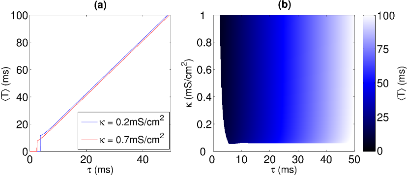
Figure 1: (color online) The interspike interval $\langle T\rangle$ for the spiking of one of the two delay-coupled standard Hodgkin-Huxley neurons with no external constant current stimulus, i.e. $I_{\mathrm{ext}}=0$, as function of the delay time $\tau$ for coupling strength $\kappa=0.2\,\mathrm{mS/cm^{2}}$ in panel (a) and as function of both parameters of the delay-coupling, i.e. the coupling strength $\kappa$ and the delay time $\tau$, in panel (b). The color encoding for the phase diagram in panel (b) is shown in the color bar: the darker the color the shorter is the interspike interval $\langle T\rangle$. For white regions, the mean interspike interval $\langle T\rangle$ tends to infinity and no repitive firing is observed.

For $I_{\mathrm{ext}}=0$, i.e. for a subthreshold constant current driving, the resulting mean interspike interval $\langle T\rangle$ is depicted in Fig. 1(a). For the coupling parameters taken within the white region of Fig. 1(b), the system relaxes to the non-spiking rest state. However, in the regime of the spiking dynamics a spike in any of the two neurons generates a subsequent spike in the other neuron. Consequently, repetitive, but alternating, firing can be observed for both neurons. The mean interspike interval $\langle T\rangle$ increases linearly with increasing delay time $\tau$, cf. Fig. 1(a). In particular,

$$\langle T\rangle\approx 2(T_{\mathrm{act}}+\tau)\,,$$ (21)

where $T_{\mathrm{act}}\approx 2\mathrm{ms}$ is the activiation time which is the time between the time the stimulus of delayed coupling sets in and the occurrence of the stimulated spiking. The factor ‘$2$’  in Eq. (21) is due to the alternating spiking of the two neurons. Note, that the time between succeeding spiking events of the network is the delay time plus the activation time.

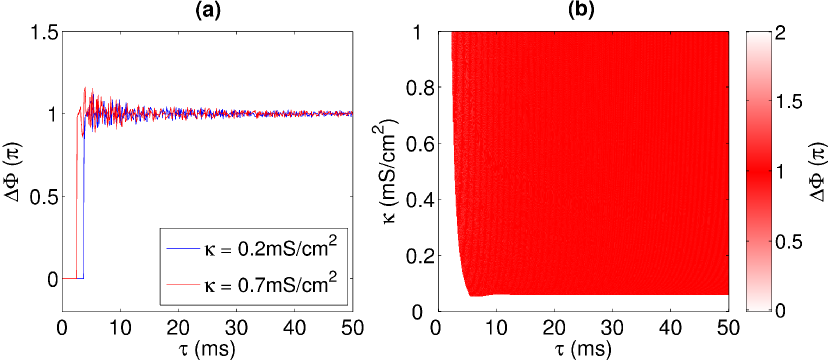
Figure 2: (color online) The phase difference $\Delta\Phi$, cf. Eq. (20), for two delay-coupled standard Hodgkin-Huxley neurons for $I_{\mathrm{ext}}=0$, cf. Eqs. (2.1)-(11), is depicted as function of the delay time $\tau$ in panel (a). In panel (b) the phase difference $\Delta\Phi$ is depicted within a phase diagram upon varying the two coupling parameters $\kappa$ and $\tau$. In the white region, there is no repetitive firing, cf. Fig. 1. In the red region the two neurons fire alternatingly, resulting in a phase difference of $\Delta\Phi\simeq\pi$.

In Fig. 2 the steady-state phase difference $\Delta\Phi$ is depicted as function of the coupling strength $\kappa$ and the delay time $\tau$. For large delay times $\tau$ the neuronal dynamics of an individual neuron possesses after each spiking event sufficient time to relax back to its rest state before the delayed stimulus caused by the spiking event of the other neuron sets in. This results in an alternating firing dynamics of the two neurons. The spiking of the two neurons therefore exhibits a constant phase shift of $\pi$, i.e. the spiking event of one neuron is almost perfectly located between two succeeding spiking events in the other neuron. However, for delay times that are of the order, or are even smaller than the refractory time, an irregular behavior of the Hodgkin-Huxley dynamics emerges, as it is to be expected in presence of finite delay. This in turn is reflected in the numerically evaluated phase difference $\Delta\Phi$ by a noisy behavior that succeedingly smoothes for increasing large delay times, yielding the afore mentioned asymptotic phase shift of $\pi$. This result is corroborated with our numerics, as depicted with Fig. 2.

3.2 Influence of channel noise

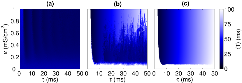
Figure 3: (color online) The interspike interval $\langle T\rangle$ for the spiking of one of the two delay-coupled standard Hodgkin-Huxley neurons with no external constant current stimulus, i.e. $I_{\mathrm{ext}}=0$, as function of the coupling parameters $\kappa$ and the delay time $\tau$. The mean interspike interval $\langle T\rangle$ is depicted for three different strengths of the channel noise: (a) strong intrinsic channel noise with $N_{\mathrm{Na}}=360\,,\quad N_{\mathrm{K}}=120$, (b) moderate intrinsic channel noise with $N_{\mathrm{Na}}=3600\,,\quad N_{\mathrm{K}}=1200$ and (c) weak intrinsic channel noise with $N_{\mathrm{Na}}=36000\,,\quad N_{\mathrm{K}}=12000$.

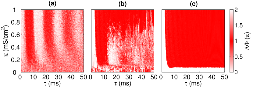
Figure 4: (color online) The steady-state phase difference $\Delta\Phi$ for two delay-coupled stochastic Hodgkin-Huxley neurons for $I_{\mathrm{ext}}=0$ is depicted as function of the delay coupling parameters $\kappa$ and $\tau$ for three different noise strengths: (a) strong intrinsic channel noise with $N_{\mathrm{Na}}=360\,,\quad N_{\mathrm{K}}=120$, (b) moderate intrinsic channel noise with $N_{\mathrm{Na}}=3600\,,\quad N_{\mathrm{K}}=1200$ and (c) weak intrinsic channel noise with $N_{\mathrm{Na}}=36000\,,\quad N_{\mathrm{K}}=12000$. The stripes in panel (a) indicate noise-induced phase-flips, see text.

In Fig. 3 we depict the dependence of the mean interspike interval $\langle T\rangle$ on the coupling parameter $\kappa$ and delay time $\tau$ for three different levels of channel noise, i.e. different sets of ion channel numbers $N_{\mathrm{Na}}$ and $N_{\mathrm{K}}$. With increasing noise level, i.e. decreasing number of ion channels, the sharp transition between the parameter regime of repetitive spiking and non-repetitive spiking is smeared out.

In addition, for considerable strong channel noise, distinct synchronization patterns emerge, indicating a frequency locking similar to the one observed for the autaptic case discussed in Sec. 4 below. In order to analyze the observed synchronization patterns in greater detail, we depict the mean interspike interval $\langle T\rangle$ as function of the delay time $\tau$ for a fixed coupling strength $\kappa=0.7\,\mathrm{mS/cm^{2}}$ in Fig. 5(a). We find that the mean interspike interval varies with the delay time in an almost piecewise linear manner, displaying sharp, triangle-like textures.

The distinct peak locations of the mean interspike interval $\langle T\rangle$ can be explained by the number of spikes that match in accordance with the intrinsic time $T_{\mathrm{intrinsic}}$ a full propagation time length, given by twice the delay time. The mean interspike interval $\langle T\rangle$ henceforth is proportional to the ratio of twice the delay time and the number of spikes fitting into this very delay time interval, cf. Eq. (21). Accordingly, channel noise results in a stabilization of the interspike interval to an interval around the intrinsic time scale of the Hodgkin-Huxley oscillator.

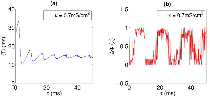
Figure 5: (color online) In panel (a) the mean interspike interval $\langle T\rangle$ is depicted as function of the coupling time $\tau$ for constant coupling strength $\kappa$, $I_{\mathrm{ext}}=0$ and channel noise level corresponding to numbers of ion channel: $N_{\mathrm{Na}}=360$ and $N_{\mathrm{K}}=120$. For the same parameters, the phase difference $\Delta\Phi$ as function of the delay time $\tau$ is depicted in (b).

3.3 Phase-flip bifurcation

Note, that this phenomenon complies with similar pattern appearing in the diagram for the phase difference, cf. Fig. 4. Furthermore, we depict the phase difference $\Delta\Phi$ in Fig. 5(b). These sharp transitions are accompanied by pronounced noise-induced phase-flips. At the corresponding phase-flip values at $0$ and $\pi$ the spiking of the basic network changes from an in-phase towards an anti-phase spiking: For $\Delta\Phi\approx 0$, both neurons spike simultaneously, implying synchronous firing, cf. Fig. 6.

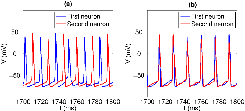
Figure 6: (color online) The simulated time-course of the membrane potentials for the two delayed coupled Hodgkin-Huxley neurons is depicted: (a) for the parameters $\kappa=0.7{\mathrm{mS/cm}}^{2}$ and $\tau=8\mathrm{ms}$,the dynamics shows alternating, i.e. antiphase, spiking, (b) for $\kappa=0.7\mathrm{mS/cm}^{2}$ and $\tau=15\mathrm{ms}$ synchronous, inphase firing of the two neurons is observed.

4 Retrospect: Frequency locking by an autaptic feedback loop

The observed frequency stabilization in the dynamics of a network of two delayed coupled neurons shares it’s origin with the frequency locking phenomenon in noisy neurons with an autaptic feedback-loop. When neuronal dendrites establish an autapse, i.e. a connection to the neuron’s own axon, a delayed feedback loop is induced to the neuron’s dynamics. Such autosynapses, described originally by Van der Loos and Glaser in 1972 [3] are a common phenomenon found in about $80\%$ of all analyzed pyramidal cells in the cerebral neocortex of human brain [4].

Auto-synapses establish a time-delayed feedback mechanism on the cellular level [3]. From a mathematical point of view, autaptic connections introduce new time scales into the single neuron dynamics which gives raise to peculiar frequency looking behavior [29]. Our modelling, cf. Eqs. (2.1)-(12), captures the stochastic autapse phenomena for $i=j$ and only one neuron.

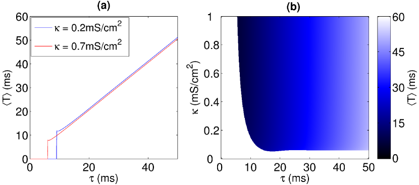
Figure 7: (color online) The interspike interval $\langle T\rangle$ for the standard Hodgkin-Huxley neuron with an autaptic feedback loop, cf. Eqs. (2.1)-(11). In panel (a) the dependence of the interspike interval $\langle T\rangle$ on the delay time $\tau$ is depicted for different coupling strengths $\kappa$. In the regime of repetitive firing the mean interspike interval $\langle T\rangle$ grows linearly with the delay time $\tau$. In the phase diagram shown in panel (b) the dependence of the interspike interval $\langle T\rangle$ on the coupling strength $\kappa$ and the delay time $\tau$ is depicted. The color bar next to panel (b) gives the color encoding for the values of the interspike intervals. The white region corresponds to the situation for which the externally initialized spike is not echoing itself and, formally, $\langle T\rangle\to\infty$.

In the limit of vanishing channel noise by letting $N_{\mathrm{Na}}\to\infty$ and $N_{\mathrm{K}}\to\infty$, the spiking period is given by the delay time $\tau$ plus the activation time $T_{\mathrm{act}}$, being the time needed for creating the next spike event after the delayed stimulus did set in, cf. Fig. 7(a). Note, that in presence of the autaptic delay, the fixed-point solution of the unperturbed Hodgkin-Huxley dynamics remains stable and the delayed stimulus is excitatory.

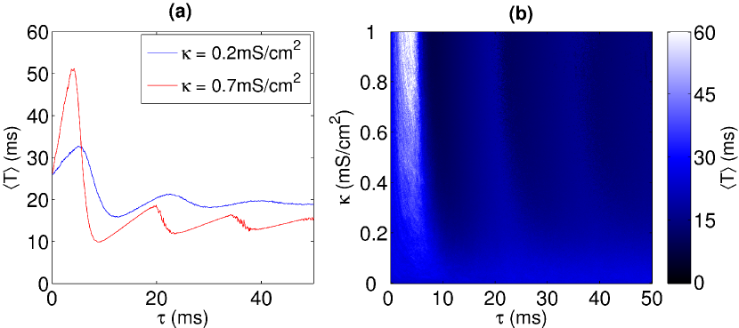
Figure 8: (color online) The mean interspike interval $\langle T\rangle$ for the stochastic Hodgkin-Huxley neuron with an autaptic feedback loop, cf. Eqs. (2.1)-(15). The channel noise level corresponds to $N_{\mathrm{Na}}=360$ and $N_{\mathrm{K}}=120$. Similarly to Fig. 7, $\langle T\rangle$ is shown as function of the delay time $\tau$ in panel (a), and the corresponding phase diagram is depicted in panel (b). The color bar gives the color encoding of the mean interspike intervals $\langle T\rangle$.

In presence of finite channel noise, however, there are two competitive mechanisms at work: (i) there are spiking repetitions due to the delay-coupling and (ii) noise-induced generation of spikes or (iii) noise-induced skipping of spikes. The interplay between these mechanisms becomes evident when the distribution of the interspike intervals is considered. In particular, the interspike interval histogram (ISIH) exhibits a bimodal structure, exhibiting two peaks, see in Fig. 6 in Ref. [29]. Upon specific values of the noise strength determined by the number of ion channels and the coupling parameters $\kappa$ and $\tau$ the bimodal structure shows distinct differences: Due to first mechanism the delay coupling leads to a significant peak around the delay time $\tau$. Via the noise-induced mechanisms, the channel noise results in a broad peak around the intrinsic time scale $T_{\mathrm{intrinsic}}$.

However, for considerable strong coupling strengths the bimodal structure collapses to an unimodal one and a frequency-locking phenomena takes place. The mean interspike interval $\langle T\rangle$ becomes bounded by a finite range of values around the intrinsic time scale, but still shows a striking dependence on the delay time $\tau$, cf. Fig 8. In particular, the mean interspike interval $\langle T\rangle$ varies with the delay time $\tau$ in an almost piecewise linear manner, displaying sharp triangle-like textures, cf. Fig. 8(a) for $\kappa=0.7\,\mathrm{mS/cm^{2}}$ and $\tau>10\,\mathrm{ms}$.

5 Conclusions

With this work we have investigated the effects of intrinsic channel noise on the spiking dynamics of an elementary neuronal network consisting of two stochastic Hodgkin-Huxley neurons. In doing so, we invoked some idealistic simplifications such as the use of bilinear coupling with identical time delays and equal coupling strengths. The finite transmission time of an action potential traveling along the neuronal axon to the dendrites is the cause for the delay-coupling to the other neuron. Physically this transmission time derives from the finite length to the connecting dendrites and the finite propagation speed.

A Pyragas-like delayed feedback mechanism has been employed to model the delayed coupling. The two basic parameters for the delay-coupling are the coupling strength $\kappa$ and the delay time $\tau$. In terms of these two parameters the delayed feedback mechanism results in a periodic, repetitive firing events of the neurons.

Apart from this repetitive firing, the delay-coupling introduces intriguing time scales. Particularly, we detect a noise-induced locking of the spiking rate to the intrinsic frequency of the system. Consequently, the delayed feedback mechanism serves as a control option for adjusting the interspike intervals; this feature may be of importance for memory storage [43] and stimulus locked short-term dynamics in neuronal systems [44]. One may therefore speculate whether ubiquitous intrinsic channel noise in combination with the autapse phenomenon is constructively harvested by nature for efficient frequency filtering.

Moreover, the emergence of a correlation between the firing dynamics of the two delayed coupled neurons has been studied in terms of stochastic phase synchronization. The dynamics of two coupled Hodgkin-Huxley neurons exhibits noise-induced phase-flip bifurcations. At these phase-flip bifurcations the phase difference changes abruptly and the spiking of the neuron switches from an in-phase spiking to an anti-phase spiking, or vice versa. These phase-flips are the direct result of the influence of channel noise. The observed phase-flips thus may possibly assist the fact of a coexistence of various frequency rhythms and oscillation patterns in different parts of extended neuronal networks, as for example it is the case for the brain.

References

References

- Masoller et al. [2008] C. Masoller, M. C. Torrent, and J. García-Ojalvo, Phys. Rev. E 78, 041907 (2008).
- Kandel et al. [1991] E. R. Kandel, J. H. Schwartz, and T. M. Jessell, Principles of Neural Science, 3rd ed. (Elsevier, New York, 1991).
- Van Der Loos and Glaser [1972] H. Van Der Loos and E. M. Glaser, Brain Res. 48, 355 (1972).
- Lübke et al. [1996] J. Lübke, H. Markram, M. Frotscher, and B. Sackmann, J. Neurosci. 16, 3209 (1996).
- Pikovsky et al. [2003] A. Pikovsky, M. Rosenblum, and J. Kurths, Synchronization: A Universal Concept in Nonlinear Sciences (Cambridge University Press, Cambridge, England, 2003).
- Varela et al. [2001] F. Varela, J. P. Lachaux, E. Rodriguez, and J. Martinerie, Nat. Rev. Neurosci. 2, 229 (2001).
- Lachaux et al. [1999] J. P. Lachaux, E. Rodriguez, J. Martinerie, and F. Varela, Hum. Brain Mapp. 8, 194 (1999).
- Prasad et al. [2006] A. Prasad, J. Kurths, S. K. Dana, and R. Ramaswamy, Phys. Rev. E 74, 035204 (2006).
- Prasad et al. [2008] A. Prasad, S. K. Dana, R. Karnatak, J. Kurths, B. Blasius, and R. Ramaswamy, Chaos 18, 023111 (2008).
- Adhikari et al. [2011] B. M. Adhikari, A. Prasad, and M. Dhamala, Chaos 21, 023116 (2011).
- Lindner et al. [2004] B. Lindner, J. García-Ojalvo, A. Neimann, and L. Schimansky-Geier, Phys. Rep. 392, 321 (2004).
- Gammaitoni et al. [1998] L. Gammaitoni, P. Hänggi, P. Jung, and F. Marchesoni, Rev. Mod. Phys. 70, 223 (1998).
- Hänggi [2002] P. Hänggi, ChemPhysChem 3, 285 (2002).
- Schmid et al. [2001] G. Schmid, I. Goychuk, and P. Hänggi, Europhys. Lett. 56, 22 (2001).
- Jung and Shuai [2001] P. Jung and J. W. Shuai, Europhys. Lett. 56, 29 (2001).
- Lacasta et al. [2002] A. M. Lacasta, F. Sagués, and J. M. Sancho, Phys. Rev. E 66, 045105(R) (2002).
- Callenbach et al. [2002] L. Callenbach, P. Hänggi, S. J. Linz, J. A. Freund, and L. Schimansky-Geier, Phys. Rev. E 65, 051110 (2002).
- Freund et al. [2003] J. A. Freund, L. Schimansky-Geier, and P. Hänggi, Chaos 13, 225 (2003).
- White et al. [2000] J. A. White, J. T. Rubinstein, and A. R. Kay, Trends Neurosci. 23, 131 (2000).
- Goldwin and Shea-Brown [2011] J. H. Goldwin and E. Shea-Brown, PLOS Comput. Biol. 7, e1002247 (2011).
- Wainrib et al. [2012] G. Wainrib, M. Thieullen, and K. Pakdaman, J. Comput. Neursci. 32, 327 (2012).
- Chow and White [1996] C. C. Chow and J. A. White, Biophys. J. 71, 3013 (1996).
- Ochab-Marcinek et al. [2009] A. Ochab-Marcinek, G. Schmid, I. Goychuk, and P. Hänggi, Phys. Rev. E 79, 011904 (2009).
- Schmid et al. [2002] G. Schmid, I. Goychuk, and P. Hänggi, Physica A 325, 165 (2002).
- Casado [2003] J. M. Casado, Phys. Lett. A 310, 400 (2003).
- Casado and Baltanás [2003] J. M. Casado and J. P. Baltanás, Phys. Rev. E 68, 061918 (2003).
- Hauschildt et al. [2006] B. Hauschildt, N. B. Janson, A. Balanov, and E. Schöll, Phys. Rev. E 74, 051906 (2006).
- Yu et al. [2007] L. Yu, Y. Chen, and P. Zhang, Eur. Phys. J. B 59, 249 (2007).
- Li et al. [2010] Y. Li, G. Schmid, P. Hänggi, and L. Schimansky-Geier, Phys. Rev. E 82, 061907 (2010).
- Hodgkin and Huxley [1952] A. L. Hodgkin and A. F. Huxley, J. Physiol. 117, 500 (1952).
- Pyragas [1992] K. Pyragas, Phys. Lett. A 170, 421 (1992).
- Nelson [2005] P. Nelson, Biological Physics (W. H. Freeman and Company, New York, 2005).
- Hassard [1978] B. Hassard, J. Theor. Biol. 71, 401 (1978).
- Rinzel and Miller [1980] J. Rinzel and R. N. Miller, Math. Biosci. 49, 27 (1980).
- Schmid et al. [2003] G. Schmid, I. Goychuk, and P. Hänggi, Lect. Notes Phys. 625, 195 (2003).
- Izhikevich [2000] E. M. Izhikevich, Int. J. Bifurcat. Chaos 10, 1171 (2000).
- Tuckwell [1987] H. C. Tuckwell, J. Theor. Biol. 127, 427 (1987).
- Fox and Lu [1994] R. F. Fox and Y. Lu, Phys. Rev. E 49, 3421 (1994).
- Hänggi and Thomas [1982] P. Hänggi and H. Thomas, Phys. Rep. 88, 207 (1982).
- Schmid and Hänggi [2007] G. Schmid and P. Hänggi, Math. Biosci. 207, 335 (2007).
- Kloeden et al. [1994] P. E. Kloeden, E. Platen, and H. Schurz, Numerical solution of SDE through computer experiments (Springer, Berlin, 1994).
- Box and Muller [1958] G. E. P. Box and M. E. Muller, Ann. Math. Stat. 29, 610 (1958).
- Seung [2000] H. S. Seung, J. Comput. Neurosci. 9, 171 (2000).
- Tass [2002] P. A. Tass, Europhys. Lett. 59, 199 (2002).