Relaxation Dynamics of Disordered Spin Chains:
Localization and the Existence of a Stationary State

Abstract

We study the unitary relaxation dynamics of disordered spin chains following a sudden quench of the Hamiltonian. We give analytical arguments, corroborated by specific numerical examples, to show that the existence of a stationary state depends crucially on the spectral and localization properties of the final Hamiltonian, and not on the initial state. We test these ideas on integrable one-dimensional models of the Ising or $XY$ class, but argue more generally on their validity for more complex (nonintegrable) models.

Ergodicity is a fundamental concept of classical mechanics: the properties of dynamical trajectories in phase space determine the long-time dynamics of a system and the description of the eventual stationary state in terms of statistical mechanics. The extension of these ideas to the quantum realm, pioneered in 1929 by J. von Neumann von Neumann (1929, 2010), has motivated a great deal of recent research, mainly spurred by the experimental possibility of studying the nonequilibrium dynamics of thermally isolated quantum systems – most notably cold atomic gases in optical lattices Bloch et al. (2008); Lewenstein et al. (2007). A highly debated issue in the recent literature is the characterization of the long-time dynamics of a quantum system taken out of equilibrium by a sudden change of one of its parameters (a quantum quench). If an extensive amount of energy is suddenly injected in the system, will the resulting dynamics tend always to a well defined stationary state? And what is the statistical ensemble describing it?

The stationary state existence, has been investigated both in generic systems von Neumann (1929) and in Hubbard-type models Cramer et al. (2008); Cramer and Eisert (2010); Flesch et al. (2008). A fast dynamical relaxation was recently observed experimentally Trotzky et al. (2012) in a system of cold atoms and its long-time stationary state results were compatible with the generalized Gibbs ensemble (GGE) Jaynes (1957); Rigol et al. (2006), where a set of macroscopic constants of motion are constrained by the initial state. Once a stationary state is established, the integrability or nonintegrability of the dynamics appears to be the crucial ingredient: while integrable systems in the thermodynamic limit are often described by a GGE Barthel and Schollwöck (2008); Calabrese et al. (2011); Cazalilla et al. (2012), it is generally expected that the breaking of integrability will lead to thermalization Rigol et al. (2008).

While the relaxation dynamics of uniform systems is well understood, recent studies hinted towards nontrivial effects due to the breaking of translational invariance. In the debate two features emerged: the importance of distinguishing between thermodynamic limit Calabrese et al. (2011); Cazalilla et al. (2012) and finite-size effects Gangardt and Pustilnik (2008); Caneva et al. (2011), and the possible role played by localization Khatami et al. (2012). For example, while breaking translational invariance in the initial state could introduce correlations among different constants of motion, relevant for finite-size systems Gangardt and Pustilnik (2008); Caneva et al. (2011), their effect has been argued to be negligible in predicting the stationary state attained by local observables Cazalilla et al. (2012). While in the thermodynamic limit the breaking of translational invariance may not have a significant effect, localization could in turn play an important role, to the extent of resulting in the absence of thermalization even in nonintegrable spin chains Khatami et al. (2012). This observation appears to be consistent with earlier numerical analysis in disordered Ising or $XY$ spin chains (characterized by localization of the eigenstates), where a discrepancy between the expected GGE and the effective stationary state was observed Caneva et al. (2011).

The purpose of this work is to characterize the long-time dynamics of disordered systems focusing on the existence of a stationary state for local observables. We do so by studying the time fluctuations of local observables in disordered spin chains which can be mapped to free fermionic systems. On the basis of analytical calculations, corroborated by numerics, we argue that the existence of a stationary state depends crucially on the spectral properties of the final Hamiltonian, and not on the initial state. While for final Hamiltonians with a continuous spectrum associated to delocalized states a well defined stationary state is attained (in the thermodynamic limit), in systems with localized states (possessing a pure-point local spectrum) time-fluctuations of local observables persist. This will be generally associated to a failure of the GGE in describing long-time averages of many-body operators. While we have tested these ideas on integrable Ising or $XY$ models, we will argue for their validity for more complex (nonintegrable) systems.

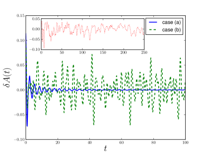
Figure 1: Illustration of the two possible behaviors for the time-dependence of an operator $A(t)$, showing the fluctuations around the time average, which decrease [case (a)] or persist at all times [case (b)]. Case (a) is a quench between disorder-free Ising chains ($h_{0}=0.9$, $h_{f}=0.5$), and case (b) a quench from a disorder-free to a disordered $XX$ chain (with $\epsilon=0.3$, see text for details). The inset shows an ambiguous case: a quench from a disordered to a clean $XX$ chain. In all cases, $\hat{A}=\hat{c}_{j}^{\dagger}\hat{c}_{j}$, the local fermionic density operator.

Let us start by defining the problem. Consider a standard quantum quench: an initial state $|\psi_{0}\rangle$, ground state of some Hamiltonian $\hat{H}_{0}$, evolves under a different time-independent Hamiltonian $\hat{H}$. Given an observable $\hat{A}$, its average can be separated in two terms:

$$A(t)\equiv\langle\psi_{0}|e^{i\hat{H}t}\hat{A}e^{-i\hat{H}t}|\psi_{0}\rangle=\bar{A}+\delta A(t)\,,$$ (1)

where $\bar{A}\equiv\lim_{T\to\infty}\frac{1}{T}\int_{0}^{T}\!dt\;A(t)$ is its time average and $\delta A(t)$ is the fluctuating part. Denoting by $|\alpha\rangle$ the eigenstates of $\hat{H}$ with energy $E_{\alpha}$, and defining $C_{\alpha}\equiv\langle\alpha|\psi_{0}\rangle$ and $A_{\alpha^{\prime}\alpha}\equiv\langle\alpha^{\prime}|\hat{A}|\alpha\rangle$, we get

$$A(t) = \sum_{\alpha}|C_{\alpha}|^{2}A_{\alpha\alpha}+\sum_{\alpha^{\prime}\neq\alpha}e^{i(E_{\alpha^{\prime}}-E_{\alpha})t}C_{\alpha^{\prime}}^{*}A_{\alpha^{\prime}\alpha}C_{\alpha}$$

$$= \left<\hat{A}\right>_{\mathrm{D}}+\int_{-\infty}^{+\infty}\!\!\!d\Omega\,e^{-i\Omega t}F_{A}(\Omega)\,,$$

where $\left<\hat{A}\right>_{\mathrm{D}}$ is the so-called diagonal average von Neumann (1929, 2010); Rigol et al. (2008) which coincides with $\overline{A}$ (assuming no energy degeneracies), and the fluctuating part $\delta A(t)$ has been recast as the Fourier transform of a weighted joint density of states $F_{A}(\Omega)\equiv\sum_{\alpha^{\prime}\neq\alpha}C_{\alpha^{\prime}}^{*}A_{\alpha^{\prime}\alpha}C_{\alpha}\delta\left(\Omega-E_{\alpha}+E_{\alpha^{\prime}}\right)$. The behavior of the fluctuating part $\delta A(t)$ (see Fig. 1) decaying to 0 for large $t$, case (a), or remaining finite (with persistent oscillations), case (b), is strongly tied to the smoothness of $F_{A}(\Omega)$. If the many-body spectrum $\{E_{\alpha}\}$, in the thermodynamic limit, is a smooth continuum and the weights $C_{\alpha^{\prime}}^{*}A_{\alpha^{\prime}\alpha}C_{\alpha}$ make $F_{A}(\Omega)$ still integrable, then $\delta A(t)$ will decay to zero for large $t$, due to the destructive interference induced by the strongly oscillating phase $e^{-i\Omega t}$ (Riemann-Lebesgue lemma). If, on the contrary, $\{E_{\alpha}\}$ has an important pure-point spectrum part, i.e., delta functions associated to localized eigenstates, then one should expect persistent time fluctuations for certain operators.

To exemplify the previous general arguments, we consider specific quenches for Hamiltonians of the Ising or $XY$ type in one dimension:

$$\hat{H}=-\sum_{j=1}^{L}\left(J_{j}^{x}\hat{\sigma}^{x}_{j}\hat{\sigma}^{x}_{j+1}+J_{j}^{y}\hat{\sigma}^{y}_{j}\hat{\sigma}^{y}_{j+1}\right)-\sum_{j=1}^{L}h_{j}\hat{\sigma}_{j}^{z}\;,$$ (2)

where $L$ is the size of the chain, $\hat{\sigma}_{j}^{\mu}$ ($\mu=x,y,z$) are Pauli matrices at site $j$ with $\hat{\sigma}_{L+1}^{\mu}\equiv\hat{\sigma}_{1}^{\mu}$. $J_{j}^{x}$, $J_{j}^{y}$ and $h_{j}$ are nearest-neighbor spin couplings and transverse magnetic fields. By a Jordan-Wigner transformation Lieb et al. (1961) $\hat{H}$ can be rewritten as a quadratic form of fermionic operators $\hat{c}_{j}$, and through a Bogoliubov rotation we define a new set of fermionic operators which diagonalize $\hat{H}$ Lieb et al. (1961); Pfeuty (1970). Wick’s theorem allows us to express $A(t)$ in terms of sums of products of one-body Green’s functions ${G}_{j_{1}j_{2}}(t)\equiv\langle\psi(t)|\hat{c}^{\dagger}_{j_{1}}\hat{c}_{j_{2}}|\psi(t)\rangle$ and ${F}_{j_{1}j_{2}}(t)\equiv\langle\psi(t)|\hat{c}^{\dagger}_{j_{1}}\hat{c}^{\dagger}_{j_{2}}|\psi(t)\rangle$. Therefore, establishing that ${G}_{j_{1}j_{2}}(t)$ and ${F}_{j_{1}j_{2}}(t)$ approach a well-defined limit for large $t$ (i.e., their fluctuations decay) allows us to make similar statements for a large class of operators, including spin-spin correlations $\hat{\sigma}^{x}_{j_{1}}\hat{\sigma}^{x}_{j_{2}}$, $\hat{\sigma}^{z}_{j_{1}}\hat{\sigma}^{z}_{j_{2}}$, and many others which may be local or nonlocal in terms of the $\hat{c}_{i}$ fermions. The case of quenches in a homogeneous Ising chain ($J_{j}^{x}=1$, $J_{j}^{y}=0$), with $h_{j}=h_{0}$ in $\hat{H}_{0}$, and $h_{j}=h_{f}\neq h_{0}$ in $\hat{H}$, is simple to illustrate: for $L\to\infty$, we have $\delta G_{j_{1}j_{2}}(t)=C\int_{0}^{\pi}\!\frac{dk}{2\pi}\frac{\cos\left[(j_{1}-j_{2})k\right]\sin^{2}k}{\epsilon_{k,{\rm f}}^{2}\epsilon_{k,{\rm 0}}}\cos\left(2\epsilon_{k,{\rm f}}t\right)$, where $C\equiv 4(h_{0}-h_{f})$ and $\epsilon_{k,{\rm 0/f}}\equiv\sqrt{1+2h_{\rm 0/f}\cos k+h^{2}_{\rm 0/f}}$ are the quasiparticle energies for $\hat{H}_{0}$ and $\hat{H}$. Case (a) of Fig. 1 is an illustration for $j_{1}=j_{2}$ (the local density), where fluctuations decay to 0 as $t^{-{3/2}}$ with oscillations Suzuki et al. (2009). This follows from the continuous single-particle spectrum and from the Riemann-Lebesgue lemma. A similar statement holds for $j_{1}\neq j_{2}$ and for $F_{j_{1}j_{2}}(t)$.

Now we turn to disordered Hamiltonians. To simplify the presentation we focus on quenches for transverse-field $XX$ chains, $J^{x}_{j}=J^{y}_{j}$, where BCS terms are absent. When disorder is present, simple analytical expressions are lacking, while pure numerics leads to ambiguous results. Figure 1, for instance, shows results for $\delta G_{jj}(t)$ upon quenching from a clean $\hat{H}_{0}$ (with $J^{x}_{j}=J^{y}_{j}=1$ and $h_{j}=0$) to a disordered $\hat{H}$ with $J_{j}^{x}=J_{j}^{y}=1+\epsilon\eta_{j}$, $h_{j}=\epsilon\xi_{j}$ and $\epsilon=0.3$ ($\epsilon$ sets the disorder strength and $\eta_{j}$, $\xi_{j}$ are uncorrelated uniform random numbers in $[-1,1[$). In this case, the fluctuations of $G_{jj}(t)$ are quite clearly persisting at all times. The inset of Fig. 1, however, shows results obtained from the opposite quench (from a disordered $\hat{H}_{0}$ to a clean $\hat{H}$), and the result for $\delta G_{jj}(t)$ is now much more ambiguous (we prove below that fluctuations decrease to 0 in such a case). To make progress we need a quantitative discrimination of the persistence of fluctuations and we introduce the mean squared fluctuations of $G_{j_{1}j_{2}}(t)$:

$$\delta_{j_{1}j_{2}}^{2}\equiv\lim_{T\rightarrow\infty}\frac{1}{T}\int_{0}^{T}\mathrm{d}t\left|\delta G_{j_{1}j_{2}}(t)\right|^{2}\;,$$ (3)

which is $0$ when time fluctuations of $G_{j_{1}j_{2}}(t)$ vanish [case (a)], and finite if they persist [case (b)]. Physically, $\delta_{jj}^{2}$ is the average fluctuation of the local density $\hat{c}_{j}^{\dagger}\hat{c}_{j}$. Let us denote by $\hat{c}^{\dagger}_{\mu}=\sum_{j=1}^{L}u_{j\mu}\hat{c}^{\dagger}_{j}$ the fermionic operators diagonalizing $\hat{H}$ and with $\epsilon_{\mu}$ their energy. If $\hat{H}$ is translationally invariant then $\mu$ is the momentum $k$ and $u_{jk}=e^{ikj}/\sqrt{L}$, while if $\hat{H}$ is disordered $u_{j\mu}$ are localized eigenfunctions. By expanding the $\hat{c}_{j}$’s in terms of the $\hat{c}_{\mu}$’s, we get $G_{j_{1}j_{2}}(t)=\sum_{\mu_{1}\mu_{2}}e^{i(\epsilon_{\mu_{1}}-\epsilon_{\mu_{2}})t}u^{\ast}_{j_{1}\mu_{1}}u_{j_{2}\mu_{2}}G_{\mu_{1}\mu_{2}}$, where $G_{\mu_{1}\mu_{2}}=\langle\psi_{0}|\hat{c}^{\dagger}_{\mu_{1}}\hat{c}_{\mu_{2}}|\psi_{0}\rangle$. Assuming no energy degeneracy (i.e., $\epsilon_{\mu_{1}}=\epsilon_{\mu_{2}}$ only if $\mu_{1}=\mu_{2}$) $\delta G_{j_{1}j_{2}}(t)$ has the same expression as $G_{j_{1}j_{2}}(t)$, except for the absence of the terms with $\mu_{1}=\mu_{2}$. The integrand in Eq. (3) is therefore

$$\begin{split}\left|\delta G_{j_{1}j_{2}}(t)\right|^{2}=\sum_{\mu_{1}\neq\mu_{2}}\sum_{\mu_{3}\neq\mu_{4}}e^{i(\epsilon_{\mu_{1}}-\epsilon_{\mu_{2}}-\epsilon_{\mu_{3}}+\epsilon_{\mu_{4}})t}\\ u^{\ast}_{j_{1}\mu_{1}}u_{j_{2}\mu_{2}}u_{j_{1}\mu_{3}}u_{j_{2}\mu_{4}}^{\ast}G_{\mu_{1}\mu_{2}}G_{\mu_{3}\mu_{4}}^{\ast}\;.\end{split}$$

With the further assumption of no gap degeneracy (i.e., $\epsilon_{\mu_{1}}-\epsilon_{\mu_{2}}=\epsilon_{\mu_{3}}-\epsilon_{\mu_{4}}$ only if $\mu_{1}=\mu_{3}$ and $\mu_{2}=\mu_{4}$, or $\mu_{1}=\mu_{2}$ and $\mu_{3}=\mu_{4}$) Rei we arrive at the key result

$$\delta_{j_{1}j_{2}}^{2}=\sum_{\mu_{1}\neq\mu_{2}}|u_{j_{1}\mu_{1}}|^{2}|u_{j_{2}\mu_{2}}|^{2}|G_{\mu_{1}\mu_{2}}|^{2}\;,$$ (4)

expressing $\delta_{j_{1}j_{2}}^{2}$ for a single realization as an eigenfunction-weighted sum of $|G_{\mu_{1}\mu_{2}}|^{2}$. Disorder averages are performed after computing $\delta^{2}_{j_{1}j_{2}}$, because we want to analyze the fluctuations of a given realization (averaging $\delta G_{j_{1}j_{2}}(t)$ would cancel such fluctuations). Notice that, while eigenfunction properties are buried in the $C_{\alpha}$ and $A_{\alpha\alpha^{\prime}}$ factors appearing in $F_{A}({\Omega})$, a many-body theory of fluctuations starting directly from $F_{A}({\Omega})$ is difficult Rei .

The nature of the eigenfunctions (localized versus extended) plays a crucial role in Eq. (4). Regardless of disorder, the $|G_{\mu_{1}\mu_{2}}|^{2}$’s sum to the total number of fermions $N_{\mathrm{F}}^{0}$ in the initial state:

$$\sum_{\mu_{1}\mu_{2}}|\langle\psi_{0}|\hat{c}^{\dagger}_{\mu_{1}}\hat{c}_{\mu_{2}}|\psi_{0}\rangle|^{2}=N_{\mathrm{F}}^{0}\;.$$ (5)

Therefore, if the final eigenstates are extended, $|u_{j_{1}\mu_{1}}|^{2}|u_{j_{2}\mu_{2}}|^{2}\sim 1/L^{2}$, then $\delta_{j_{1}j_{2}}^{2}$ in (4) scales to zero as $N_{\mathrm{F}}^{0}/L^{2}\sim 1/L$ for a system with a finite density of fermions. If $\hat{H}$ is clean we have to take care of the degeneracy $\epsilon_{k}=\epsilon_{-k}$ and the particle-hole symmetry, but still, see supplementary material (SM), we can prove a bound $\delta^{2}_{j_{1}j_{2}}\leq 8N_{\mathrm{F}}^{0}/L^{2}$, indicating that fluctuations vanish for $L\to\infty$. This generalizes the result of Ref. Cazalilla et al. (2012) to cases where $\hat{H}_{0}$ might lead to a $|G_{k_{1}k_{2}}|^{2}$ which has important nonvanishing contributions also for $k_{1}\neq k_{2}$ (see SM).

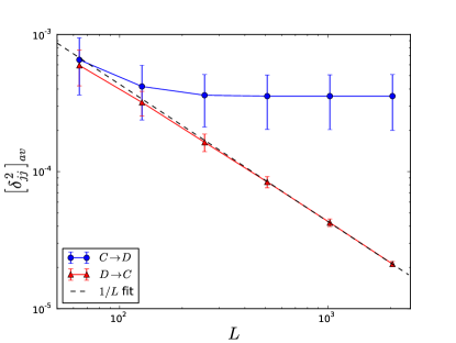
Figure 2: Average values of $\delta^{2}_{jj}$ with $j=L/2$, Eqs. (3) and (4), for quenches of $XX$ chains when $|\psi_{0}\rangle$ is the ground state of a disordered $\hat{H}_{0}$ (with $\epsilon=0.3$), while $\hat{H}$ is clean with $h_{j}=0$ (triangles $D\rightarrow C$), or the opposite case (circles $C\rightarrow D$), see text for details. The averages are taken over $200$ different disordered realizations and the error bar is the standard deviation of the distribution (not the error on the average).

Figure 2 shows the disorder average $[\delta^{2}_{jj}]_{av}$ as a function of $L$ in the two opposite situations described above, i.e., quenches from a disordered $\hat{H}_{0}$ to a clean $\hat{H}$ ($D\to C$), or vice versa ($C\to D$). In all cases $\delta^{2}_{jj}$ is calculated from Eq. (4) (with the extra terms due to degeneracies in the $D\to C$ case). When $\hat{H}$ is clean ($D\to C$ data), $[\delta^{2}_{jj}]_{av}$ scales to $0$ as $1/L$ , as expected from the bound discussed below Eq. 5. On the contrary, when $\hat{H}$ is disordered ($C\to D$ data), $[\delta^{2}_{jj}]_{av}$ converges unambiguously to a nonvanishing quantity for $L\to\infty$: time fluctuations survive at all times when $\hat{H}$ is disordered. This is in full agreement with the numerical results  Gramsch and Rigol (2012) obtained for the density after a quench into the localized phase of the Aubry-André model in one dimension. For smaller disorder amplitude $\epsilon$, the situation is similar, except that the large-$L$ plateau occurs for larger $L$, due to larger localization lengths.

To better gauge the role of the localized eigenfunctions in making $\delta^{2}_{j_{1}j_{2}}$ finite for $L\to\infty$, we have analyzed histograms of the quantities appearing in Eq. (4). A histogram of $|G_{\mu_{1}\mu_{2}}|^{2}$ shows that while the average of $|G_{\mu_{1}\mu_{2}}|^{2}$ scales to zero as $1/L$, see Eq. (5), the distribution of its values has large tails. To analyze these tails, we work with logarithmic distributions, and define

$$P_{j_{1}j_{2}}^{w}(x)\equiv\sum_{\mu_{1}\neq\mu_{2}}\frac{|u_{j_{1}\mu_{1}}|^{2}|u_{j_{2}\mu_{2}}|^{2}}{\mathcal{N}_{j_{1}j_{2}}}\delta\left(x-\log\left|G_{\mu_{1}\mu_{2}}\right|^{2}\right)\,$$ (6)

where $\mathcal{N}_{j_{1}j_{2}}\equiv\sum_{\mu_{1}\neq\mu_{2}}|u_{j_{1}\mu_{1}}|^{2}|u_{j_{2}\mu_{2}}|^{2}=1-\sum_{\mu}|u_{j_{1}\mu}|^{2}|u_{j_{2}\mu}|^{2}$ is a normalization constant, $0<\mathcal{N}_{j_{1}j_{2}}<1$, related to the inverse participation ratio H. Aoki, J. Phys. C: Solid State Phys., 16, 205, .() (1983) when $j_{1}=j_{2}$.

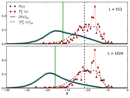
Figure 3: Plot of $P^{w}_{jj}(x)$, Eq. (6) with $j=L/2$ (triangles), and $P(x)$, Eq. (7) (circles), for $XX$ chain quenches from a clean $\hat{H}_{0}$ (with $h_{j}=0$) to a disordered $\hat{H}$ (with $\epsilon=0.3$), for two values of the chain length $L$. $[P^{w}_{j_{1}j_{2}}(x)]_{av}$ and $[P(x)]_{av}$ (dashed and solid lines) are averages over different realizations of disorder, with the corresponding vertical lines indicating their mean values $\int\!\mathrm{d}x\,x[P^{w}_{j_{1}j_{2}}(x)]_{av}$ and $\int\!\mathrm{d}x\,x[P(x)]_{av}$.

Figure 3 shows $P_{jj}^{w}(x)$ for two different sizes, and compares it with the unweighted distribution

$$P(x)\equiv\frac{1}{L(L-1)}\sum_{\mu_{1}\neq\mu_{2}}\delta\left(x-\log\left|G_{\mu_{1}\mu_{2}}\right|^{2}\right)\;.$$ (7)

We plot both single-instance distributions (solid points) as well as disorder average distributions $[\cdots]_{av}$, denoted by lines. The unweighted distribution $P(x)$ is smooth, and self-averaging, and moves towards smaller mean values when $L$ increases. On the contrary, $P_{jj}^{w}(x)$ is more structured (single-instance distributions depend on the details of the weights $|u_{j_{1}\mu_{1}}|^{2}|u_{j_{2}\mu_{2}}|^{2}$), but its mean does not decrease with $L$, due to an eigenfunction reweighting of rare events with large values of $|G_{\mu_{1}\mu_{2}}|^{2}$. Physically, this is quite transparent: similarly to what happens for the inverse participation ratio H. Aoki, J. Phys. C: Solid State Phys., 16, 205, .() (1983), localized eigenstates are rather insensitive to the size, while extended states are. The fact that the mean $\int\!\mathrm{d}x\,xP^{w}_{j_{1}j_{2}}(x)$, remains finite for $L\to\infty$ for almost all realizations, is enough to conclude that $\delta^{2}_{j_{1}j_{2}}$ stays finite in the disordered $\hat{H}$ case. Indeed, Jensen’s inequality implies $\delta^{2}_{j_{1}j_{2}}={\mathcal{N}_{j_{1}j_{2}}}\langle e^{x}\rangle_{P_{j_{1}j_{2}}^{w}}\geq{\mathcal{N}_{j_{1}j_{2}}}e^{\langle x\rangle_{P_{j_{1}j_{2}}^{w}}}$ and $\mathcal{N}_{j_{1}j_{2}}$ remains finite when $L\to\infty$.

We have shown that microscopic operators have persistent fluctuations after a quench to a disordered $\hat{H}$. Such fluctuations could be averaged out if one considers extensive operators involving sums over all sites. For instance, in a quench to a final disordered Ising chain, while the local transverse magnetization $\sigma^{z}_{j}(t)=2G_{jj}(t)-1$ has persistent fluctuations, the corresponding extensive operator, the total transverse magnetization (per site) $\hat{m_{z}}=L^{-1}\sum_{j}\hat{\sigma}^{z}_{j}$, has fluctuations which decrease to $0$ as $L$ is increased, as we have verified. Physically, extensive operators effectively perform a self-averaging of the fluctuations $\delta A(t)$, which then vanish in the $L\to\infty$ limit. Again, this agrees with the numerical results of Ref. Gramsch and Rigol (2012).

Let us comment on the issue of thermalization, namely if an ensemble exists which is able to describe long-time averages of Ising or $XY$ chains. One can prove Ziraldo and Santoro (2012) that for one-body operators (like $G_{j_{1}j_{2}}(t)$ and $F_{j_{1}j_{2}}(t)$), independently of the size — even finite — and of the quench, time averages coincide with the corresponding GGE average: this result can be traced back to the constraints imposed by the GGE. Thanks to the Wick’s expansion, GGE averages reproduce the time averages for any $\hat{A}$ that can be expressed as a finite linear combination of powers of $\hat{c}_{j}$ and $\hat{c}^{\dagger}_{j}$, as long as the time-fluctuations of $G_{j_{1}j_{2}}(t)$ and $F_{j_{1}j_{2}}(t)$ vanish. On the contrary, when the disorder makes the fluctuations of $G_{j_{1}j_{2}}(t)$ and $F_{j_{1}j_{2}}(t)$ persistent, the time-averages of many-body operators might in general differ from their GGE value. We have verified that this is the case, for instance, for $\hat{\sigma}^{z}_{j}\hat{\sigma}^{z}_{j+r}$ in quenches from a clean to a disordered $XX$ chain. These results are in agreement with the numerical findings of Ref. Gramsch and Rigol (2012).

In conclusion, we have shown that the spectral properties and the localization or delocalization of the eigenstates of the final Hamiltonian play an important role in characterizing the time fluctuations of observables. While the observations we made are based on the analysis of quenches of an integrable Hamiltonian we expect that the structure of $F_{A}(\Omega)$ is what ultimately governs the fluctuations: integrability should not be crucial in this respect. The fact that, in our one-dimensional models, disorder localizes all eigenstates is also likely not crucial. For fermions hopping in a three-dimensional Anderson model, where there is a mobility edge separating localized and delocalized eigenstates, Eq. (4) is still valid, and we expect that localized eigenstates contribute a finite quantity to $\delta^{2}_{j_{1}j_{2}}$ in the thermodynamic limit. Both these issues, however, clearly call for future investigations.

We thank F. Becca, M. Fabrizio, J. Marino, G. Menegoz, A. Russomanno, and P. Smacchia for discussions. Research was supported by SNSF, through SINERGIA Project No. CRSII2 136287 1, by the EU-Japan Project LEMSUPER, and by the EU FP7 under Grant Agreement No. 280555.

References

- von Neumann (1929) J. von Neumann, Z. Phys. 57, 30 (1929).
- von Neumann (2010) J. von Neumann, Eur. Phys. J. H 35, 201 (2010).
- Bloch et al. (2008) I. Bloch, J. Dalibard, and W. Zwerger, Rev. Mod. Phys. 80, 885 (2008).
- Lewenstein et al. (2007) M. Lewenstein, A. Sanpera, V. Ahufinger, B. Damski, A. Sende, and U. Sen, Advances in Physics 56, 243 (2007).
- Cramer et al. (2008) M. Cramer, A. Flesch, I. P. McCulloch, U. Schollwöck, and J. Eisert, Phys. Rev. Lett. 101, 063001 (2008).
- Cramer and Eisert (2010) M. Cramer and J. Eisert, New J. Phys. 12, 055020 (2010).
- Flesch et al. (2008) A. Flesch, M. Cramer, I. P. McCulloch, U. Schollwöck, and J. Eisert, Phys. Rev. A 78, 033608 (2008).
- Trotzky et al. (2012) S. Trotzky, Y.-A. Chen, A. Flesch, I. P. McCulloch, U. Schollwöck, J. Eisert, and I. Bloch, Nature Phys. 8, 325 (2012).
- Jaynes (1957) E. T. Jaynes, Phys. Rev. 108, 171 (1957).
- Rigol et al. (2006) M. Rigol, A. Muramatsu, and M. Olshanii, Phys. Rev. A 74, 053616 (2006).
- Barthel and Schollwöck (2008) T. Barthel and U. Schollwöck, Phys. Rev. Lett. 100, 100601 (2008).
- Calabrese et al. (2011) P. Calabrese, F. H. L. Essler, and M. Fagotti, Phys. Rev. Lett. 106, 227203 (2011).
- Cazalilla et al. (2012) M. A. Cazalilla, A. Iucci, and M.-C. Chung, Phys. Rev. E 85, 011133 (2012).
- Rigol et al. (2008) M. Rigol, V. Dunjko, and M. Olshanii, Nature 452, 854 (2008).
- Gangardt and Pustilnik (2008) D. M. Gangardt and M. Pustilnik, Phys. Rev. A 77, 041604 (2008).
- Caneva et al. (2011) T. Caneva, E. Canovi, D. Rossini, G. E. Santoro, and A. Silva, JSTAT p. P07015 (2011).
- Khatami et al. (2012) E. Khatami, M. Rigol, A. Relaño, and A. M. Garcia-Garcia, Phys. Rev. E 85, 050102 (2012).
- Lieb et al. (1961) E. Lieb, T. Schultz, and D. Mattis, Annals of Physics 16, 407 (1961).
- Pfeuty (1970) P. Pfeuty, Annals of Physics 57, 79 (1970).
- Suzuki et al. (2009) S. Suzuki, D. Rossini, and G. E. Santoro, ArXiv e-prints (2009), eprint 0910.4055.
- (21) Using a nondegeneracy condition for the gaps, while often reasonable for single-particle energies, is dangerous for many-body energies. This would lead to the incorrect result that fluctuations are always negligibly small, as discussed in P. Reimann, Phys. Rev. Lett. 101, 190403 (2008).
- Gramsch and Rigol (2012) C. Gramsch and M. Rigol, Phys. Rev. A 86, 053615 (2012).
- H. Aoki, J. Phys. C: Solid State Phys., 16, 205, .() (1983) H. Aoki, J. Phys. C: Solid State Phys., 16, 205, (1983).
- Ziraldo and Santoro (2012) S. Ziraldo and G. E. Santoro, ArXiv e-prints (2012), eprint 1211.4465.