INTERACTION    BETWEEN    AN    ISOTROPIC
NANOPARTICLE AND DRIFTING ELECTRONS
IN A QUANTUM WELL

Abstract

A hybrid system composed of an isotropic nanoparticle and a semiconductor heterostructure with a quantum well has been considered. The nanoparticle is supposed to be polarizable in an external electric field. A theoretical model of the hybrid system is substantiated and formulated. Exact solutions of the model equations are obtained. The frequencies of charge oscillations in the hybrid system and their damping owing to the dipole–plasmon interaction are found, the damping mechanism being similar to that of Landau damping. The space-time behavior of concentration perturbations in the two-dimensional electron gas is analyzed, and the polarization oscillations of a nanoparticle are studied. The induced polarization of a nanoparticle at nonzero electron drift velocities is found to have a complicated dynamics. In particular, the polarization vector circulates along elliptic trajectories for two of three frequency dispersion branches. If the electric current flows through the quantum well due to an applied electric field, the damping of oscillations in the hybrid system is replaced by their growth in time, which corresponds to the electric instability of the system. New phenomena in hybrid systems can be used to excite the emission of nanoparticles by an electric current and to electrically stimulate the emission in the terahertz spectral range.

1 Introduction

Physical phenomena in the terahertz (THz) spectral range are intensively studied, which is associated with the fundamental importance of new terahertz physics, as well as with a considerable number of feasible applications. In particular, many researches aim at constructing new sources and detectors of THz radiation.

In this context, of great interest are the researches of semiconductor heterostructures with quantum wells (QWs), in which collective oscillations of a two-dimensional electron gas (2DEG), i.e. plasmons, can be excited. The frequencies of plasmon oscillations belong to the THz spectral range. In a homogeneous 2DEG, plasmons are stable, i.e. their oscillations attenuate in time owing to the electron scattering by various crystal defects and by means of the known mechanism of Landau damping. Various methods were proposed in order to achieve the instability and obtain oscillation-growth effects intended to be used for the amplification and the generation of THz radiation. Among those, a possibility of the instability excitation owing to the electron drift in an electric field [1,​ 2,​ 3], various variants of two-beam instability [3,​ 4], and others were examined. However, for such instabilities to be realized in a spatially uniform plasma, very high drift velocities, which are difficult to be obtained experimentally, are required. The situation essentially changes in spatially non-uniform or finite systems [5]. For example, as was shown in works [6], if special types of contacts are applied to a quantum well with a finite length, the electron system becomes unstable already at moderate drift velocities of electrons. This instability has been studied experimentally [7,​ 8,​ 9].

Another class of objects, which are active in the THz spectral range, includes quantum dots [10,​ 11,​ 12,​ 13], molecules and some molecular compounds [14,​ 15,​ 16], shallow impurity centers [17,​ 18,​ 19], and so forth. For brevity, let us call such “zero-dimensional” objects as nanoparticles (NPs).

Hybrid systems consisting of nanoparticles and heterostructures with free electrons constitute a new type of heterodimensional objects, which should demonstrate essentially new properties and effects. In particular, if the oscillation frequencies of zero-dimensional NPs and two-dimensional plasmons are in the THz spectral range, hybrid systems may reveal new properties at extremely high frequencies. Therefore, the study of the interaction between such NPs and plasmons under equilibrium and nonequilibrium conditions seems well-timed.

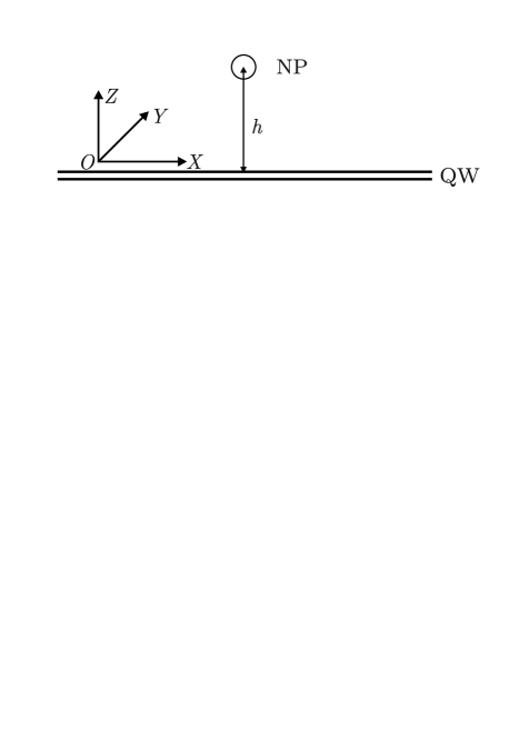
Fig. 1.: Schematic drawing of the hybrid system. The $OY$ axis is perpendicular to the figure plane

In work [20], the studies of the interaction between a remote nanoparticle and a drifting 2DEG at relatively low frequencies, i.e. when the application of the “low-frequency” drift-diffusion approximation is valid, were started. In this work, we present the results of our researches of THz-frequency properties of hybrid systems in the “high-frequency” approximation for the electron motion in a 2DEG. We revealed collective oscillations of interacting nanoparticles and the 2DEG. In particular, we determined the frequencies of collective oscillations and their extra damping stemming from the interaction between the nanoparticle and plasmons. The damping character is similar to that of Landau damping. This system was demonstrated to become unstable under definite nonequilibrium conditions, i.e. there emerges an increase of collective oscillations in time induced by an electric current. The nanoparticle destroys the translational symmetry, and the system becomes non-uniform, which promotes the appearance of an instability, similarly to what takes place in non-uniform or spatially confined plasma [5].

The structure of the paper is as follows. In Section 2, the model of a hybrid system is discussed, and the basic equations are substantiated. In Section 3, the exact solutions of the equations are obtained, and their general properties are examined. In Section 4, the main attention is given to the stability/instability of a hybrid system under the condition of two-dimensional electron drift, the numerical results are presented, and the specific examples of nanoparticles and heterostructures with two-dimensional electrons are considered. The features of coordinated space-time charge waves are dealt in Section 5. The properties of the NP dipole moment, plasmon field, and emission by the hybrid system are studied in Section 6. Conclusions are presented in Section 7.

2 Model and Basic Equations

Consider a hybrid system represented schematically in Fig. 1. It consists of a spherical nanoparticle, which can be polarized in an external field, and the heterostructure with a quantum well, in which two-dimensional electrons are localized. The distance between the nanoparticle and the quantum well is $h$. The electrons and the nanoparticle interact by means of the electrostatic field $\mathbf{E}=-\mathbf{\nabla}\phi$, where $\phi(x,y,z,t)$ is a self-consistent electrostatic potential. The latter is described by the Poisson equation

$$\frac{\kappa}{4\pi}\Delta\phi=e({n}-n_{0})\delta(z)+\left({\ \mathbf{D}}(t)\mathbf{\nabla}\right)\delta(x)\delta(y)\delta(z-h),$$ (1)

where $\kappa$ is the dielectric permittivity, $e$ the electron charge, ${n}(x,y,t)$ the surface concentration of electrons, $n_{0}$ the equilibrium surface concentration of electrons, $\mathbf{D}(t)$ the electric dipole moment of a nanoparticle, and $\delta(x)$ the Dirac delta-function.

It is convenient to express the scalar potential as a sum of two terms associated with the electrons and the NP, ${\phi(x,y,z,t)=\phi_{e}(x,y,z,t)+\phi_{d}(x,y,z,t)}$, where $\phi_{e}$ and $\phi_{d}$ are determined from the system of equations

$$\begin{cases}\displaystyle{\kappa\Delta\phi_{e}=4\pi e({n}-n_{0})\delta(z),}\cr\displaystyle{\kappa\Delta\phi_{d}=4\pi\left({\mathbf{D}}(t)\mathbf{\nabla}\right)\delta(x)\delta(y)\delta(z-h).}\end{cases}$$ (2)

To describe electrons in the quantum well (the plane $z=0$), we use Euler’s equation of motion and the continuity equation, which couple the surface concentration ${n}(x,y,t)$ and the electron velocity $\mathbf{\mathfrak{v}}(x,y,t)$ with the electrostatic field. In the general case, we assume that electrons move with an average drift velocity $\mathbf{v_{0}}$. Then, the equations are [6]

$$\begin{cases}\displaystyle{\frac{\partial\mathbf{\mathfrak{v}}}{\partial t}+\left({\mathbf{\mathfrak{v}}}{\mathbf{\nabla}}_{\parallel}\right){\mathbf{\mathfrak{v}}}=\left.\frac{e}{m}\mathbf{\nabla}\phi\right|_{z=0}-\frac{\mathbf{\mathfrak{v}-v_{0}}}{\tau_{p}}}\,,\cr\displaystyle{\frac{\partial{n}}{\partial t}+{\mathbf{\nabla}}_{\parallel}\left(\mathbf{\mathfrak{v}}{n}\right)=0}\,,\end{cases}$$ (3)

where $m^{\ast}$ is the effective mass of an electron, the term ${\frac{\mathbf{\mathfrak{v}-v_{0}}}{\tau_{p}}}$ makes allowance for the electron scattering by crystal defects, and $\tau_{p}$ is the time of electron momentum relaxation. The subscript $\parallel$ is used for quantities and differential operators dealing with the plane $z=0$ only. For instance, the Laplace operator in the plane $z=0$ is ${\Delta_{\parallel}=\frac{\partial^{2}}{\partial x^{2}}+\frac{\partial^{2}}{\partial y^{2}}}$. At the same time, the Laplace operator in the volume is ${\Delta=\Delta_{\parallel}+\frac{\partial^{2}}{\partial z^{2}}}$. We will also mark the real and imaginary parts of complex numbers as primed quantities, e.g., ${Z=Z^{\prime}+iZ^{\prime\prime}}$.

In the two-dimensional electron gas, there emerge collective oscillations of the charge density, which are called plasmons. The hydrodynamic model with Eqs. (3) is valid, when the frequency of these oscillations, $\omega$, and the absolute value of the wave vector, $k$, satisfy the conditions

$$\omega\tau_{p}\gg 1,\,\,ql_{p}\sim l_{p}/h\gg 1\,,$$ (4)

where $l_{p}$ is the mean free path of electrons. The formulation of the problem includes only one characteristic length scale; it is the distance $h$ between the plane of the 2DEG and the NP. Therefore, one may expect that the wave vectors of plasmons, which make the major contribution to the interaction between the electrons and the NP, should be of the order of $1/h$. Note that inequalities (4) correspond to the ballistic character of the electron motion in the spatial region, which is actual for the nanoparticle–plasmon interaction.

Suppose that the velocity of electrons is ${\mathbf{\mathfrak{v}}(x,y,t)=\mathbf{v_{0}}+\mathbf{v}(x,y)e^{-i\omega t}},$ and their concentration ${{n}(x,y,t)=n_{0}+n(x,y)e^{-i\omega t}}$, with ${v\ll v_{0}}$ and ${n\ll n_{0}}$. Let the time dependences of potentials also vary harmonically, i.e. ${\phi_{e}(x,y,z,t)=\varphi_{e}(x,y,z)e^{-i\omega t}}$ and ${\phi_{d}(x,y,z,t)=\varphi_{d}(x,y,z)e^{-i\omega t}}$. The frequency $\omega$ in these formulas should be determined by solving the equations; generally speaking, it is a complex-valued quantity, which corresponds to the oscillations (damped or growing in time) in the hybrid system. (If ${\omega^{\prime\prime}>0}$, the system is unstable, and ${\omega^{\prime\prime}}$ is called the instability increment.) The quantities $\mathbf{v}(x,y)$ and $n(x,y)$ describe the spatial dependences of electron velocity and concentration perturbations, respectively.

According to Fig. 1, the nanoparticle is located at the point $\left(x=0,y=0,z=h\right)$. In an external electric field, it becomes polarized and can be characterized by an electric dipole moment, which is determined by the relation

$${\mathbf{D}(t)=\mathbf{d}(\omega)e^{-i\omega t},}$$

$${\mathbf{d}(\omega)=-\left.\beta_{0}(\omega)\mathbf{\nabla}\varphi_{e}\right|_{x=y=0,z=h},}$$ (5)

where $\beta_{0}(\omega)$ is the nanoparticle polarizability. Note that formula (5) includes only the electron potential and, hence, the dipole self-action is excluded from consideration. If the nanoparticle is isotropic, its polarizability can be expressed in the standard form [21]

$${\beta_{0}(\omega)=-\sum\limits_{f}\frac{2\omega_{f}e^{\ast^{2}}}{\hbar}\,\frac{|\langle f|x|0\rangle|^{2}}{\omega^{2}-\omega_{f}^{2}+i\omega/\tau_{f}}}\,,$$ (6)

where $\hbar$ is the reduced Planck constant, $\hbar\omega_{f}$ is the energy of the $f$-th nanoparticle level, $\tau_{f}$ is the lifetime of this level, $\langle f|x|0\rangle$ is the matrix element of the dipole transition between the ground and $f$-th excited states.

The largest contribution to polarizability (6 ) is given by the transition between the ground and the first excited state. In this case, the polarization is

$${\beta_{0}(\omega)=-\frac{e^{\ast^{2}}}{\hbar}\,\frac{|\langle 1|x|0\rangle|^{2}}{\omega-\omega_{0}+i\gamma_{0}}}\,,$$ (7)

where the characteristic frequency of dipole oscillations, ${\omega_{0}}$, and the damping of dipole oscillations corresponding to the transition between the ground and the first excited state, ${\gamma_{0}=1/(2\tau_{1})}$, are introduced. While deriving formula (7), an assumption was made that $\omega$ is close to $\omega_{0}$, because the main effects are expected to take place at frequencies close to the characteristic frequency of dipole oscillations.

Equations (1)–(3), (5), and (7) compose a basic system for the problem under consideration.

3 Solutions of the Equations and Their General Properties

The dipole potential, being the solution of the second Poisson equation in system (2), has the well-known form

$${\varphi_{d}=\frac{1}{\kappa}\frac{d_{x}(\omega)x+d_{y}(\omega)y+d_{z}(\omega)(z-h)}{(x^{2}+y^{2}+(z-h)^{2})^{\frac{3}{2}}}},$$ (8)

where $d_{x}$, $d_{y}$, and $d_{z}$ are the components of the dipole moment $\mathbf{d}(\omega)$. Below, for all quantities depending on coordinates, the two-dimensional Fourier transformation is used:

$${\varphi_{e}(\mathbf{r},z)=\!\int\!d^{2}\!k\,\varphi_{k}(z)\,e^{i\mathbf{k}\mathbf{r}}},$$ (9)

$${n(\mathbf{r})=\!\int\!d^{2}\!k\,n_{k}\,e^{i\mathbf{k}\mathbf{r}}\,,\,\,\,\,\,\psi(\mathbf{r})=\!\int\!d^{2}\!k\,\psi_{k}\,e^{i\mathbf{k}\mathbf{r}},}$$ (10)

where ${\mathbf{r}=(x,y)}$, ${\mathbf{k}=(k_{x},k_{y})}$, and ${\psi(\mathbf{r})=\left.\varphi_{d}(\mathbf{r},z)\right|_{z=0}}$. The quantities $\varphi_{k}(z)$, $n_{k}$, and $\psi_{k}$ are the Fourier transforms of the electron potential, surface concentration, and potential induced by the dipole in the quantum-well plane ($z=0$), respectively. Then, the Poisson equation for $\varphi_{k}(z)$ and the required boundary conditions are

$$\begin{cases}\displaystyle{\frac{d^{2}\varphi_{k}^{\pm}}{dz^{2}}-k^{2}\varphi_{k}^{\pm}=0},\\[5.69054pt] \displaystyle{\left.\varphi_{k}^{\pm}\right|_{z\rightarrow\pm\infty}\rightarrow 0,}\\[5.69054pt] \displaystyle{\left.\varphi_{k}^{+}\right|_{z=0+\varepsilon}=\left.\varphi_{k}^{-}\right|_{z=0-\varepsilon},}\\[5.69054pt] \displaystyle{\left.\frac{d\varphi_{k}^{+}}{dz}\right|_{z=0+\varepsilon}-\left.\frac{d\varphi_{k}^{-}}{dz}\right|_{z=0-\varepsilon}=\frac{4\pi en_{k}}{\kappa},}\end{cases}$$ (11)

where $\varphi_{k}^{+}(z)=\varphi_{k}(z)$ at $z\geq 0$ and $\varphi_{k}^{-}(z)=\varphi_{k}(z)$ at $z\leq 0$, $k=\sqrt{k_{x}^{2}+k_{y}^{2}}$, and $\varepsilon\rightarrow+0$.

The solution of system (11) and the functions $\psi_{k}$ and $n_{k}$ are

$$\begin{cases}\displaystyle{\varphi_{k}=-\frac{2\pi en_{k}}{\kappa k}e^{-k|z|}}\\[5.69054pt] \displaystyle{\psi_{k}=-\frac{1}{2\pi\kappa}\left(i\frac{d_{x}k_{x}+d_{y}k_{y}}{k}+d_{z}\right)e^{-kh}}\\[8.53581pt] \displaystyle{n_{k}=-\frac{en_{0}k^{2}}{m}\frac{\left.\varphi_{k}\right|_{z=0}+\psi_{k}}{(\omega-\mathbf{v_{0}k})(\omega-\mathbf{v_{0}k}+i/\tau_{p})}}.\end{cases}$$ (12)

Note that, in the limiting case where the dipole is infinitely far from the 2DEG (i.e. ${h\rightarrow\infty}$), solutions (12) easily bring about the dispersion law for collective excitations in the drifting 2DEG, i.e. drifting plasmons,

$${\omega_{\pm}=\mathbf{v_{0}k}\pm\sqrt{\frac{2\pi e^{2}n_{0}}{\kappa m}k-\frac{\gamma_{p}^{2}}{4}}-\frac{i\gamma_{p}}{2},}$$ (13)

where the notation ${\gamma_{p}=1/\tau_{p}}$ is used. On the other hand, the zero of the denominator of $\beta_{0}(\omega)$ (Eq. (7)) corresponds to the frequency and the damping of a dipole, $\omega=\omega_{0}-i\gamma_{0}$.

If the distance $h$ is finite, system (12) and relations (5) and (7) can be used to derive an integral equation, e.g., for the Fourier transform of the concentration of electrons interacting with the dipole,

$${n_{k}=-\frac{e^{2}n_{0}}{\kappa^{2}m}\frac{\beta_{0}(\omega)ke^{-kh}(k_{x}I_{x}+k_{y}I_{y}+kI_{z})}{(\omega-\mathbf{v_{0}}\mathbf{k})(\omega-\mathbf{v_{0}}\mathbf{k}+i\gamma_{p})-\frac{2\pi e^{2}n_{0}k}{\kappa m}}},$$ (14)

where ${I_{x}}$,$\ {I_{y}}$, and ${I_{z}}$ are the functionals of $n_{k}$,

$${I_{x}\!=\!\!\!\int\!\!d^{2}q\frac{q_{x}}{q}n_{q}e^{-qh}},\,\displaystyle{I_{y}\!=\!\!\!\int\!\!d^{2}q\frac{q_{y}}{q}n_{q}e^{-qh}},\displaystyle{I_{z}\!=\!\!\!\int\!\!d^{2}qn_{q}e^{-qh}}.$$

With the notations

$${B_{0}=-\frac{e^{2}n_{0}}{\kappa^{2}m}\beta_{0}(\omega)},$$

$${\Delta_{e}(\omega,k)=(\omega-\mathbf{v}_{0}\mathbf{k})(\omega-\mathbf{v}_{0}\mathbf{k}+i\gamma_{p})-\frac{2\pi e^{2}n_{0}k}{\kappa m}},$$

the integral equation (14) yields the following system of algebraic equations:

$$\begin{cases}\displaystyle{I_{x}=B_{0}(S_{x}I_{x}+S_{0}I_{z}),}\cr\displaystyle{I_{y}=B_{0}S_{y}I_{y},}\cr\displaystyle{I_{z}=B_{0}(S_{0}I_{x}+S_{z}I_{z}),}\end{cases}$$ (15)

where the notations

$${S_{x}=\int\frac{d^{2}kk_{x}^{2}e^{-2kh}}{\Delta_{e}(\omega,k)}}\,,\displaystyle{S_{y}=\int\frac{d^{2}kk_{y}^{2}e^{-2kh}}{\Delta_{e}(\omega,k)}},$$

$${S_{z}=\int\frac{d^{2}kk^{2}e^{-2kh}}{\Delta_{e}(\omega,k)}},\,\displaystyle{S_{0}=\int\frac{d^{2}kk_{x}ke^{-2kh}}{\Delta_{e}(\omega,k)}}\,.$$ (16)

are used for the calculable integrals. Note that the parameter ${S_{0}=0}$, if the electron drift is absent ($\mathbf{v}_{0}=0$).

The zero value of the determinant of the system of equations (15) is a condition for the nontrivial solutions of the integral equation (14) to exist. This condition, which determines the frequency $\omega$, will be referred to as a dispersion equation. If the electron velocity is directed along the $OX$ axis, the dispersion equation is

$$\left[(1-B_{0}S_{x})(1-B_{0}S_{z})-B_{0}^{2}S_{0}^{2}\right]\left[1-B_{0}S_{y}\right]=0.$$ (17)

The dispersion equation (17) describes all possible collective oscillations of electrons and the dipole. If electrons are in the equilibrium state ($\mathbf{v}_{0}=0$ and $S_{0}=0$), the dispersion equation can be decomposed into three equations: $(1-B_{0}S_{x})=0$, $(1-B_{0}S_{y})=0$, and $(1-B_{0}S_{z})=0$. The solutions of each of them correspond to different orientations of the induced dipole. It is evident that the solutions of equations (the frequencies of collective dipole and electron oscillations), which correspond to the $x$- and $y$-orientations of the dipole, are identical, because these two directions are physically equivalent in the absence of charge carrier drift. The frequency of collective oscillations for the $z$-orientation of the dipole is, generally speaking, different from those corresponding to the $x$- and $y$-orientations.

In the general case, Eq. (17) is factorized into two separate equations. One of them is the equation

$${(1-B_{0}S_{x})(1-B_{0}S_{z})=B_{0}^{2}S_{0}^{2}}\,.$$

One can easily verify that, for the frequencies, which are the solutions of this equation, the electric field of electrons has a symmetry, at which the induced dipole of a nanoparticle lies in the $x-z$ plane, i.e. it corresponds to a mixed $x-z$ orientation. The roots of this equation are two frequency branches. The branch, which is associated at ${v_{0}=0}$ with the $x$-orientation of the dipole (i.e. which is determined by the equation ${B_{0}S_{x}=1}$), will be called the $x$-branch. Accordingly, the other branch will be called the $z$-branch. As it was in the equilibrium case (${v_{0}=0}$), the solutions of the equation

$${B_{0}S_{y}=1}$$

correspond to the orientation of the dipole in parallel to the $OY$ axis for any $v_{0}$-value; therefore, the corresponding frequency branch will be referred to as the $y$-branch.

The solutions of the dispersion equation (17) can be presented in the form

$$\Omega_{j}=\Omega_{0}-i\Gamma_{0}+\frac{\Lambda}{\Omega_{0}}R_{j}(V_{0},\Omega_{j},\Gamma_{p}),$$ (18)

where the subscript $j=x,y,z$ denotes the $x$-, $y$-, and $z$-branches, respectively. We also used the notations

$${\Omega_{j}=\frac{\omega_{j}}{\omega_{pl}}},\quad\displaystyle{\omega_{pl}=\sqrt{\frac{2\pi e^{2}n_{0}}{\kappa mh}}},\quad V_{0}=\frac{v_{0}}{\omega_{pl}h}\,,$$

$$\Omega_{0}=\frac{\omega_{0}}{\omega_{pl}},\quad\displaystyle{\Gamma_{0}=\frac{\gamma_{0}}{\omega_{pl}}},\quad\displaystyle{\Gamma_{p}=\frac{1}{2\gamma_{p}\omega_{pl}}},$$

$${\Lambda=\frac{e^{2}e^{*^{2}}{n}_{0}|\langle 1|x|0\rangle|^{2}}{\kappa^{2}mh^{4}\hbar\omega_{pl}^{4}}}\,.$$

The parameter $\Lambda$ is responsible for the coupling between the 2DEG and the dipole; and ${R_{j}(V_{0},\Omega_{j},\Gamma_{p})}$ is a certain complex-valued function depending on the electron drift velocity, the frequency of dipole oscillations, and the plasmon damping. For the $x$- and $z$-branches, the expressions for the functions $R_{x,z}$ are

$${R_{x,z}=\!\frac{1}{2}\!\left[S_{x}\!+\!S_{z}\!\pm(S_{x}\!-\!S_{z})\sqrt{1+\!\left(\frac{2S_{0}}{S_{x}-S_{z}}\right)^{2}}\right],\!}$$ (19)

where the plus sign corresponds to the $x$-branch, and the minus sign to the $z$-branch. It is easy to obtain a simpler expression for the $y$-branch,

$${R_{y}=S_{y}}\,.$$

The real part of this function, ${R_{j}^{\prime}}$, describes a shift of the oscillation frequency of the system with respect to the eigenfrequency of the dipole owing to the interaction between the dipole and electrons. The corresponding imaginary part, ${R_{j}^{\prime\prime}}$, is responsible for the additional damping (or growing) of oscillations in the hybrid system.

From the analysis of integrals (16), it follows that, in the extremely high-frequency case (4), the functions ${R_{j}}$ practically do not depend on the parameter $\Gamma_{p}$. (In the hydrodynamic approximation, which is used in this work, the plasmon damping is exclusively governed by the one-particle relaxation of electrons. The Landau damping for plasmons, which arises, if the electron kinetics is considered [22], is assumed small.) In the absence of electron drift, it can be shown analytically that, if ${\Gamma_{p}\rightarrow 0}$,

$${R_{x,y}}=\pi\mathcal{P}\!\!\int{dk\frac{k^{3}e^{-2k}}{\Omega_{x,y}^{2}-k}-i\pi^{2}\Omega_{x,y}^{6}e^{-2\Omega_{x,y}^{2}},}$$

$${R_{z}=2R_{x,y}}.$$ (20)

The nonzero value of ${R_{j}^{\prime\prime}}$ and, respectively, the oscillation damping (analogous to the Landau damping [22]) in the hybrid system originate from the collective interaction. Really, since the spectrum of plasmons (Eq. (13)) is continuous, for any given frequency $\omega_{0},$ there can always be found “resonance” plasmons, the charge waves of which are proportional to $\exp[i(\mathbf{k_{r}r}-\omega t)]$, where the wave vector $\mathbf{k_{r}}$ satisfies the condition $\omega^{\pm}(\mathbf{k_{r}})=\omega_{0}$. At the same time, the electric field of the dipole is a sum of Fourier components $\mathbf{E}_{d,\mathbf{k}}\exp[i\mathbf{k}\mathbf{r}-i\omega_{0}t]$, with ${\mathbf{k}=\mathbf{k}_{r}}$ inclusive. The dipole field waves with the wave vectors $\mathbf{k}_{r}$ and the “resonance” plasmons are cophased, and they propagate with the same velocity. This means that the corresponding dipole field acts permanently (without variation in time) on “resonance” plasmon charges. As a result, the work of the dipole field over the charges is nonzero, and the dipole loses its energy. Under nonequilibrium conditions, the dipole can acquire the energy from the electron subsystem. A necessary condition for that is

$${R_{j}^{\prime\prime}(V_{0},\Omega_{j},\Gamma_{p})>0\,.}$$ (21)

The sufficient condition for the hybrid system to be unstable in whole is more rigorous:

$${\frac{\Lambda}{\Omega_{0}}R_{j}^{\prime\prime}(V_{0},\Omega_{j},\Gamma_{p})>\Gamma_{0}\,,}$$ (22)

If the inverse inequality is obeyed, either the system is stable or the oscillations in the system attenuate.

Fig. 2.: Dependences of the real ($a$) and imaginary ($b$) parts of the function $R_{j}$ on the electron drift velocity at a fixed frequency of dipole oscillations (${\Omega_{0}\approx 0.58}$). The other parameters are given in the text

4 Interaction between a Shallow Donor and Drifting Two-Dimensional Electrons

In this section, we apply the results obtained above to a specific hybrid system consisting of a shallow impurity center and a heterostructure with a quantum well.

It is well known that one-particle Coulomb impurities in semiconductors are characterized by low binding energies, and the allowed photo-induced dipole transitions between impurity states correspond to the THz spectral range. Such impurities can be regarded as hydrogen-like atoms, the energy spectrum and the wave functions of which can be calculated in the effective mass approximation (see, e.g., work [23]). The energy difference between the basic, $1S$, and excited, $2P$, states is evaluated as ${E_{S-P}={3e^{2}}/{8\kappa a_{B}}}$, where ${a_{B}=\kappa\hbar^{2}/me^{2}}$ is the radius in the ground state. For example, for GaAs with ${m=0.067m_{0}}$ and ${\,\kappa=12.9}$ ($m_{0}$ is the free electron mass), we obtain ${E_{S-P}\approx 4.12\leavevmode\nobreak\ }$meV and ${a_{B}\approx 10}$ nm. This energy difference corresponds to the frequency ${\omega_{0}\approx 6.2\times 10^{12}}$ s^-1 ($\approx 0.99$ THz). The phototransition ${S\leftrightarrow P}$ is an allowed electric dipole transition with the transition matrix element ${\langle 1|x|0\rangle}\approx{0.52}\,{a_{B}^{\ast}}$. The cited parameters allow the polarizability of a Coulomb impurity to be calculated using relation (7).

To achieve conditions needed for the instability excitation, a substance for the heterostructure must be selected, which would be characterized by high electron velocities. Consider a quantum well on the basis of InAs with GaAs-barriers. It is known [24] that the effective electron mass in InAs is small, ${m\approx 0.023m_{0}}$, and the electron mobility is high even at room temperature, ${\mu\approx 8\times 10^{4}}\leavevmode\nobreak\ \mathrm{cm}^{\mathrm{2}}/(\mathrm{V\times s})$. It gives rise to very high drift velocities of electrons, up to ${v_{0}\approx 6\times 10^{7}}$ $\mathrm{cm/s}$ [24,​ 25]. In quantum wells on the basis of InGaAs, drift velocities of the same order are observed. The difference between the dielectric constants of the quantum well and the barrier can be neglected [20]. For numerical calculations, let us choose such physical parameters that criteria (4) are satisfied. In particular, let us fix the electron concentration ${n_{0}=10^{11}}\leavevmode\nobreak\ \mathrm{cm}^{-2}$ and the distance from the 2DEG to the donor ${h=4\times 10^{-6}}$ $\mathrm{cm}$. The corresponding characteristic parameters, which were introduced by relations (19), are ${\omega_{pl}\approx 1.07\times 10^{13}}$ s^-1, ${\Lambda\approx 0.0013}$, and ${\Gamma_{p}\approx 0.03}$. The drift velocity of charge carriers is normalized by the quantity ${\omega_{pl}h\approx 4.28\times 10^{7}}$ $\mathrm{cm/s}$.

Fig. 3.: Dependences of the real ($a$) and imaginary ($b$) parts of the function $R_{j}$ on the frequency $\Omega_{0}$ at the fixed electron drift velocity ${V_{0}\approx 0.94}$. The other parameters are given in the text

In Figs. 2 and 3, the dependences of the real, $R_{j}^{\prime}$, and imaginary, $R_{j}^{\prime\prime}$, parts of the function $R_{j}$ on the normalized velocity $V_{0}$ and frequency $\Omega_{0}$, respectively, are depicted. Figures 2,$a$ and 3,$a$ bring us to a conclusion that, for the selected fixed parameters, the frequency of oscillations in the system is a little (in comparison with $\omega_{0}$) shifted toward lower values in the frequency $x$- and $y$-branches, and to both sides in the $z$-branch. Figure 2 also demonstrates that $R_{x}^{\prime\prime}$ changes its sign at ${V_{0}\approx 0.8}$, which corresponds to the drift velocity ${v_{0}\approx 3.4\times 10^{7}}$ $\mathrm{cm/s}$. If condition (22) is also obeyed at that, an instability must emerge, and oscillations in the system start to grow. The figure also illustrates that the $x$- and $y$-branches merge together at low enough drift velocities, which is associated with the equivalence of those directions at ${V_{0}\rightarrow 0}$. Figure 3 testifies that the lower the frequency of dipole oscillations, the larger is the instability increment. As to the $y$- and $z$-branches, ${R_{y}^{\prime\prime}<0}$ and ${R_{z}^{\prime\prime}<0}$ in the considered ranges of frequencies and drift velocities; therefore, the corresponding oscillations in the system attenuate here.

As was shown in works [17,​ 18,​ 19], the inverse lifetime of donor electrons at shallow donors in GaAs can be of the order of $10^{7}\leavevmode\nobreak\ \mathrm{s}^{-1}$. For ${V_{0}\approx 0.94}$ and ${\Omega_{0}\approx 0.58}$, we obtain ${\frac{\Lambda}{\Omega_{0}}R_{x}^{\prime\prime}\omega_{pl}\approx 5.28\times 10^{9}}\leavevmode\nobreak\ \mathrm{s}^{-1}$. In this case, criterion (22) is satisfied well, and the indicated instability effects must be observed for the hybrid system concerned. Note that the increase in the electron concentration or the distance $h$ leads to a reduction of the instability increment, because ${\Lambda\propto n_{0}^{-1}}$ and ${\Lambda\propto h^{-2}}$. We also verified that all effects discussed depend weakly on the parameter $\Gamma_{p}$.

Therefore, using an InAs quantum well and a shallow hydrogen-like donor in the GaAs barrier as an example, we showed that an instability can take place in the $x$-branch of collective oscillations in the system. Oscillations corresponding to the $y$ and $z$ frequency branches attenuate.

5 Charge Waves

In the previous sections, the dispersion equation for collective oscillations of the dipole and the 2DEG was derived and analyzed. Its solutions are the characteristic frequencies (eigenvalues) of oscillations. In this section, we are going to construct eigenfunctions, which correspond to those eigenvalues and are the solutions of the integral equation (14). The analysis of these solutions will allow one to understand the behavior of the electron subsystem at collective oscillations.

Let us recall that the integral equation (14) for the charge carrier concentration $n_{k}$ must be specified for the corresponding type of collective oscillations, after the solutions of the system of algebraic equations (15) for $I_{x}$, $\,I_{y}$, and $\,I_{z}$ (they are functionals of $n_{k}$) have been found. For two mixed $x-z$ orientations of the dipole, the quantity $I_{y}$ is nullified. Then, using the first and third equations of this system, it is easy to obtain

$${I_{z}=K_{x}I_{x}=K_{z}^{-1}I_{x},}$$

where the notations ${K_{x}=B_{0}S_{0}/(1-B_{0}S_{z})}$ and ${K_{z}=B_{0}S_{0}/(1-B_{0}S_{x})}$ are introduced (in these notations, the dispersion equation for the $x$- and $z$-branches reads ${K_{x}K_{z}=1}$). Then, the solution of the linear integral equation (14), which corresponds to the $x$-branch of frequencies, is

$$n_{k}^{(x)}=CB_{0}\frac{k\left(k_{x}+K_{x}k\right)}{\Delta_{e}(\omega_{x},k)}e^{-kh}\,,$$ (23)

where the superscript in parentheses in the notation $n_{k}^{(x)}$ means that the frequency entering into the quantities $B_{0}$, $K_{x}$, and $\Delta_{e}$ belongs to the $x$-branch. Generally speaking, the constant $C$ is an arbitrary complex value characterized by an amplitude and a phase. The latter is insignificant, because it can always be zeroed by shifting the start of time counting. Therefore, $C$ is assumed real-valued below.

Substituting Eq. (23) into the formula of the Fourier transformation, we obtain the space-time distribution of a concentration perturbation,

$$n^{(x)}(\mathbf{r},t)=CB_{0}\int d^{2}k\frac{k\left(k_{x}+K_{x}k\right)}{\Delta_{e}(\omega_{x},k)}e^{-kh+i\mathbf{kr}-i\omega_{x}t}.$$ (24)

It is the real part of expression (24) that has a physical meaning. Let

$${J_{x}(\mathbf{r})=CB_{0}\int d^{2}k\frac{kk_{x}}{\Delta_{e}(\omega_{j},k)}e^{-kh+i\mathbf{kr}}}\,,$$

$${J_{z}(\mathbf{r})=CB_{0}\int d^{2}k\frac{k^{2}}{\Delta_{e}(\omega_{j},k)}e^{-kh+i\mathbf{kr}}}$$

and ${\tau_{j}=\omega_{j}^{\prime}t}$, where $j=x$ for the $x$-branch. Extracting the real part of the concentration perturbation (24), we obtain

$${n^{\prime\>(x)}(\mathbf{r},\tau_{x})=}$$

$$=\displaystyle{e^{\frac{\omega_{x}^{\prime\prime}}{\omega_{x}^{\prime}}\tau_{x}}\biggl{[}(J_{x}^{\prime}(\mathbf{r})+K_{x}^{\prime}J_{z}^{\prime}(\mathbf{r})-K_{x}^{\prime\prime}J_{z}^{\prime\prime}(\mathbf{r}))\cos{\tau_{x}}+}$$

$${+(J_{x}^{\prime\prime}(\mathbf{r})+K_{x}^{\prime}J_{z}^{\prime\prime}(\mathbf{r})+K_{x}^{\prime\prime}J_{z}^{\prime}(\mathbf{r}))\sin{\tau_{x}}\biggr{]}}.$$ (25)

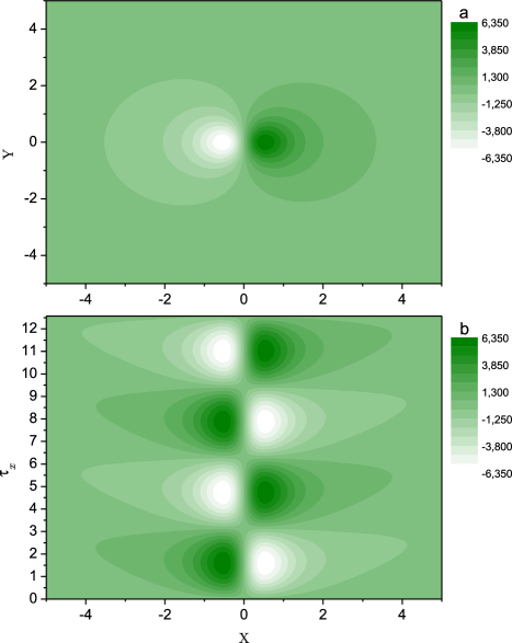
Fig. 4.: Contour plots of the space-time dependences of electron concentration perturbations at $V_{0}=0$, which correspond to the $x$-branch of frequencies: ($a$) the spatial dependence at $\tau_{x}=\frac{3\pi}{2}$, ($b$) the space-time dependence at $Y=0$

Solutions (25) have the following properties. The function $n^{\prime(x)}(\mathbf{r},\tau_{x})$, as well as $n^{(x)}(\mathbf{r},t)$, is even with respect to $y$. Since ${\frac{\omega_{x}^{\prime\prime}}{\omega_{x}^{\prime}}\ll 1}$, the amplitude of this function changes slightly within several periods. At ${V_{0}=0}$, $n^{\prime(x)}(\mathbf{r},\tau_{x})$ is an odd function of the coordinate $x$. In general, $n^{\prime(x)}(\mathbf{r},\tau_{x})$ describes the behavior of charge waves in the two-dimensional space and in time.

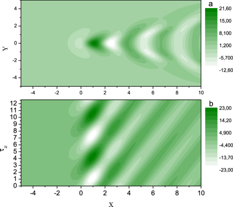
Fig. 5.: The same as in Fig. 4, but at ${V_{0}\approx 0.94}$

In Fig. 4, the contour plots of the space-time dependences of electron concentration perturbations corresponding to the $x$-branch (in this case, the dipole is oriented along the $OX$ axis) in the absence of electron drift ($V_{0}=0$) are exhibited. In particular, in Fig. 4,$a$, the spatial distribution of the concentration at the time moment ${\tau_{x}={3\pi}/{2}}$ is shown. It has a minimum and a maximum to the left and to the right, respectively, from the coordinate origin, where the dipole is located. This distribution arose owing to the corresponding arrangement of dipole charges at that moment. The time-space illustration (Fig. 4,$b$) demonstrates that those maxima and minima alternate in time with a period of $\pi$. The spatial scale of perturbations has an order of several $h$.

The contour plots of the space-time dependences of the electron concentration in the case where electrons drift along the $OX$ axis (${V_{0}\approx 0.94}$), are shown in Fig. 5. In the general case, if electrons drift, the dipole becomes oriented in the plane $y=0$ (see the next section). One can see that the concentration minima and maxima, which are exhibited in Fig. 4, are “blown” by the electron stream, with the perturbation boundaries moving faster than its center. The nonzero phase velocity of plasmon waves, which is perpendicular to the electron drift, results in a smearing of perturbations located far from the dipole.

A similar analysis of the time-space distributions of electrons can be carried out for the $z$-branch of the frequency dispersion. For this case, instead of Eq. (25), we obtain

$${n^{\prime\>(z)}(\mathbf{r},\tau_{z})=}$$

$${=e^{\frac{\omega_{z}^{\prime\prime}}{\omega_{z}^{\prime}}\tau_{z}}\biggl{[}(K_{z}^{\prime}J_{x}^{\prime}(\mathbf{r})-K_{z}^{\prime\prime}J_{z}^{\prime\prime}(\mathbf{r})+J_{z}^{\prime}(\mathbf{r}))\cos{\tau_{z}}+}$$

$${+(K_{z}^{\prime}J_{x}^{\prime\prime}(\mathbf{r})+K_{z}^{\prime\prime}J_{z}^{\prime}(\mathbf{r})+J_{z}^{\prime\prime}(\mathbf{r}))\sin{\tau_{z}}\biggr{]}}.$$ (26)

The properties of this function are a little similar to those of the function ${n^{\prime(x)}(\mathbf{r},\tau_{x})}$. In particular, this function is also even with respect to $y$. However, in contrast to ${n^{\prime(x)}(\mathbf{r},\tau_{x})}$, ${n^{\prime(z)}(\mathbf{r},\tau_{z})}$ is an even function of the coordinate $x$ at $V_{0}=0$.

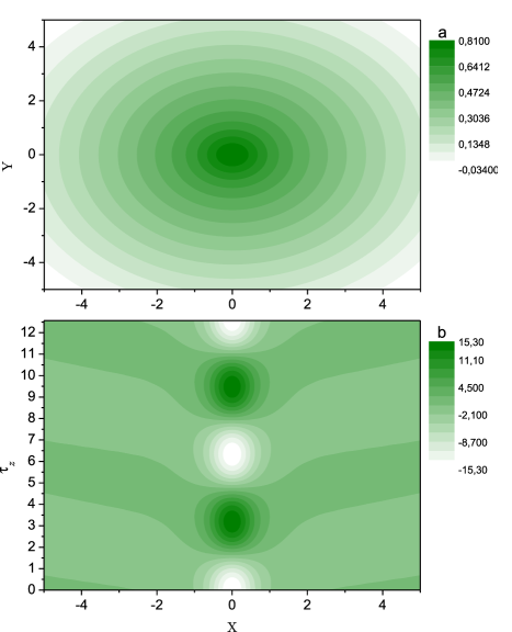
Fig. 6.: The same as in Fig. 4, but for the $z$-branch

Figure 6 illustrates the behavior of the electron concentration for the $z$-branch of frequencies at ${V_{0}=0}$ (the dipole is oriented along the $OZ$ axis). The spatial distribution of the electron concentration calculated for the time moment ${\tau_{x}={3\pi}/{2}}$ (see Fig. 6,$a$) has a maximum, which is located under the dipole and is symmetric with respect to the substitutions ${x\rightarrow-x}$ and ${y\rightarrow-y}$. Figure 6,$b$ demonstrates the behavior of a perturbation in time, which is close to periodic. Figure 7 exhibits the same as in Fig. 6, but provided that electrons drift with the velocity ${V_{0}\approx 0.94}$. In this case, the dipole is also oriented in the plane $y=0$, but the wave dynamics is somewhat more complicated than that obtained above for the $x$-branch. Perturbations located near the dipole move against the electron stream, whereas the remote perturbations move along the stream. At ${X\approx 3.5}$, the character of perturbations changes, and the role of the wave propagation becomes dominant.

Consider the solution of the integral equation (14) for the dipole $y$-orientation. The real part of an electron concentration perturbation looks like

$${n^{\prime(y)}(\mathbf{r},\tau_{y})=e^{\frac{\omega_{y}^{\prime\prime}}{\omega_{y}^{\prime}}\tau_{y}}\left[J_{y}^{\prime}(\mathbf{r})\cos{\tau_{y}}+J_{y}^{\prime\prime}(\mathbf{r})\sin{\tau_{y}}\right]},$$ (27)

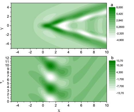
Fig. 7.: The same as in Fig. 5, but for the $z$-branch

where the notation

$${J_{y}(\mathbf{r})=CB_{0}\int d^{2}k\frac{kk_{y}}{\Delta_{e}(\omega_{y},k)}e^{-kh+i\mathbf{kr}}}$$

is used. The properties of $n^{\prime(y)}(\mathbf{r},\tau_{y})$ are also similar with to those of $n^{\prime(x)}(\mathbf{r},\tau_{x})$. At ${V_{0}=0}$, the frequency branches coincide; therefore, in order to derive $n^{\prime(y)}(\mathbf{r},\tau_{y})$ from $n^{\prime(x)}(\mathbf{r},\tau_{x}),$ the substitution ${X\leftrightarrow Y}$ should be made. The same concerns Fig. 4 as well. In contrast to $n^{\prime(x)}(\mathbf{r},\tau_{x})$, $n^{\prime(y)}(\mathbf{r},\tau_{y})$ is an odd function of the coordinate $y$ for an arbitrary $V_{0}$, which is connected with a constant orientation of the dipole in parallel to the $OY$ axis. Figure 8 illustrates the coordinate (panel $a$) and coordinate-time (panel $b$) dependences of the electron concentration perturbation, which corresponds to the $y$-branch at the electron drift. At ${Y=0}$, the integrand in the integral $J_{y}(\mathbf{r})$ is an odd function, so that ${n^{\prime(y)}(x,y=0,\tau_{y})=0}$. Therefore, Fig. 8 was plotted for $y=0.5$. It can be interpreted like Fig. 7,$b$: perturbations are blown down the electron streams; however, in this case, perturbation minima transform into maxima and vice versa.

Hence, in this section, we determined the behavior of perturbations in the two-dimensional electron gas in the hybrid system for various types of solutions, which takes into account whether or not the electrons drift.

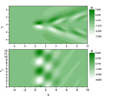
Fig. 8.: The same as in Fig. 5, but for the $y$-branch at $Y=0.5$

6 Behavior of the Dipole Induced in a Nanoparticle

Consider the behavior of the nanoparticle polarization during collective electric oscillations in the hybrid system. This behavior is described by the dynamics of the induced dipole moment (5). To determine the dipole moment, we have to calculate the electric field created by electrons at the dipole localization point making use of definition (9), the first formula in system (12), and the Fourier components of the concentration $n_{k}$ (the latter were analyzed for various dispersion branches in the previous section).

First, let us consider the solutions corresponding to the dispersion $x$-branch, provided that the components of the dipole moment are

$$\begin{cases}\displaystyle{d_{x}(\omega_{x})=-iC\frac{2\pi e\beta_{0}(\omega_{x})}{\kappa}\equiv\widetilde{C}_{x}},\cr\displaystyle{d_{y}(\omega_{x})=0,}\cr\displaystyle{d_{z}(\omega_{x})=i\widetilde{C}_{x}K_{x}},\end{cases}$$ (28)

where $\widetilde{C}_{x}$ is a new arbitrary constant. Whence, we obtain the law for the time evolution of dipole moment components,

$$\begin{cases}\displaystyle{D_{x}=e^{\frac{\omega_{x}^{\prime\prime}}{\omega_{x}^{\prime}}\tau_{x}}(\widetilde{C}_{x}^{\prime}\cos\tau_{x}+\widetilde{C}_{x}^{\prime\prime}\sin\tau_{x}),}\cr\displaystyle{D_{z}=-e^{\frac{\omega_{x}^{\prime\prime}}{\omega_{x}^{\prime}}\tau_{x}}\left[(\widetilde{C}_{x}^{\prime}K_{x}^{\prime\prime}+\widetilde{C}_{x}^{\prime\prime}K_{x}^{\prime})\cos\tau_{x}+\right.}\cr\displaystyle{+\left.(\widetilde{C}_{x}^{\prime\prime}K_{x}^{\prime\prime}-\widetilde{C}_{x}^{\prime}K_{x}^{\prime})\sin\tau_{x}\right]}.\end{cases}$$ (29)

System (29) is a parametric equation of an ellipse: the end of the dipole moment vector moves along an elliptic trajectory in the plane $y=0$. It is easy to verify that ${K_{x}^{\prime}>0}$ and ${K_{x}^{\prime\prime}>0}$ for the $x$-branch of the frequency dispersion; hence, this circulation is counter-clockwise. Since the dipole is in a self-consistent field with drifting electrons, the parameters of this ellipse depend on the drift velocity and the frequency of dipole oscillations.

Let us put the arbitrary constant ${\widetilde{C}_{x}=1}$ and, for simplicity, let $\exp\left(\frac{\omega_{x}^{\prime\prime}}{\omega_{x}^{\prime}}\tau_{x}\right)\approx{1}$, i.e. we consider the behavior of the system within several periods. Then,

$$\begin{cases}\displaystyle{D_{x}=\cos\tau_{x},}\cr\displaystyle{D_{z}=K_{x}^{\prime}\sin\tau_{x}-K_{x}^{\prime\prime}\cos\tau_{x}}.\end{cases}$$ (30)

After excluding the parameter $\tau_{x}$ from system (30), we obtain the equation for this ellipse in the form

$${aD_{x}^{2}+2bD_{x}D_{z}}+cD_{z}^{2}=1,$$ (31)

where ${a=1+\left({K_{x}^{\prime\prime}}/{K_{x}^{\prime}}\right)^{2}}$, ${b={K_{x}^{\prime\prime}}/{K_{x}^{\prime^{2}}}}$, and ${c={1}/{K_{x}^{\prime^{2}}}}$. The rotation of the coordinate system by an angle $\alpha_{x}$ determined by the equation

$${\tan\alpha_{x}=\frac{1-K_{x}^{\prime^{2}}-K_{x}^{\prime\prime^{2}}}{2K_{x}^{\prime\prime}}\pm\sqrt{\left(\frac{1-K_{x}^{\prime^{2}}-K_{x}^{\prime\prime^{2}}}{2K_{x}^{\prime\prime}}\right)^{2}+1}}\,,$$ (32)

brings about the canonical ellipse equation,

$${\frac{D_{x_{0}}^{2}}{A^{2}}+\frac{D_{z_{0}}^{2}}{B^{2}}=1,}$$ (33)

where $D_{x_{0}}$ and $D_{z_{0}}$ are the dipole components in the new coordinate system, and $A$ and $B$ are the principal ellipse axes,

$${A^{2}=\frac{1+\operatorname{tg}^{2}\alpha_{x}}{a+2b\operatorname{tg}\alpha_{x}+c\,\operatorname{tg}^{2}\alpha_{x}}},$$

$${B^{2}=\frac{1+\operatorname{tg}^{2}\alpha_{x}}{a\operatorname{tg}^{2}\alpha_{x}-2b\operatorname{tg}\alpha_{x}+c}}\,.$$ (34)

The parameters $A$ and $B$ are used to introduce the ellipse eccentricity,

$${\epsilon=}\begin{cases}\displaystyle{\sqrt{1-\frac{B^{2}}{A^{2}}},\;\;A>B,}\\[5.69054pt] \displaystyle{\sqrt{1-\frac{A^{2}}{B^{2}}},\;\;A<B}.\end{cases}$$ (35)

Fig. 9.: Dependences of ($a$) the ellipse eccentricity $\epsilon_{j}$ and ($b$) the rotation angle $\alpha_{j}$ (in degree units) of the principal axes of the ellipse on the electron drift velocity

The ${\epsilon}$-magnitude varies from zero to 1. The ellipse transforms into a circle at ${\epsilon\rightarrow 0}$ and into a line at ${\epsilon\rightarrow 1}$. The eccentricity of the ellipse, along which the dipole circulates, evidently depends on the electron drift velocity and the frequency of dipole oscillations, because the principal axes depend on $K_{x}$.

Note that the time dependence of the dipole is very simple in the coordinate system coupled with the principal axes, namely,

$$\begin{cases}\displaystyle{D_{x_{0}}=A\cos\tau_{x},}\cr\displaystyle{D_{z_{0}}=B\sin\tau_{x}.}\end{cases}$$ (36)

Similar formulas can also be derived for solutions associated with the dispersion $z$-branch. In this case, the dipole also circulates along an ellipse, but now “clockwise”. The principal axes of this ellipse depend on $K_{z}(\omega_{z})$. To obtain the canonical ellipse equation for the $z$-branch, the substitutions ${a\leftrightarrow c}$, ${b\rightarrow-b}$, and ${K_{x}(\omega_{x})\rightarrow-K_{z}(\omega_{z})}$ should be made in the equations written above. Now, the eccentricity is described by expression (35), but the principal axes swap (${A\leftrightarrow B}$), and the angle ${\alpha_{x}}$ changes to ${\alpha_{z}}$. The eccentricity is the same for both dispersion branches, because ${K_{x}(\Omega_{x})\simeq-K_{z}(\Omega_{z})}$.

Concerning the $y$-orientation of the dipole, the eccentricity of the corresponding ellipse is equal to 1 for all $V_{0}$, which is associated with the dipole orientation strictly along the $OY$ axis for any $V_{0}$.

The dependences of eccentricity $\epsilon$ on the electron drift velocity for three different dipole oscillation frequencies are depicted in Fig. 9,$a$. The solid curve exposes the eccentricity that corresponds to the same frequency as in all previous figures, where this frequency was fixed, i.e. ${\Omega_{0}\approx 0.58}$. Two other curves correspond to half as high and twice as high dipole oscillation frequencies. The figure testifies that the eccentricity is equal to 1, if the drift velocity equals zero, i.e. the dipole oscillates with the frequency $\Omega_{x}$ along the $OX$ axis and with the frequency $\Omega_{z}$ along the $OZ$ axis. Figure 9,$b$ shows that the lines, along which the dipole oscillates, are perpendicular to each other at ${V_{0}=0}$. If $V_{0}$ increases, the eccentricity decreases, and the line transforms into an ellipse. The ellipse, which corresponds to the $x$-branch, rotates “clockwise”; therefore, the absolute value of the angle, by which its axes are rotated with respect to the $OX$ axis, grows. The other ellipse rotates “counter-clockwise”; therefore, the absolute value of its orientation angle decreases. At a certain drift velocity, those ellipses coincide.

A similar situation takes place at other dipole oscillation frequencies as well. The curves in Fig. 9 also demonstrate that the eccentricities have a similar structure at different frequencies, and the smallest $\epsilon$-value is realized for a curve that corresponds to ${\Omega_{0}\approx 0.58}$. At this frequency, the function $R_{j}$, the plot of which is exhibited in Fig. 2, changes drastically in a vicinity of the drift velocity, which corresponds to the eccentricity minimum (${V_{0}\approx 0.43}$). The plots of the functions $\alpha_{x}$ and $\alpha_{z}$ intersect each other also in a vicinity of ${V_{0}\approx 0.43}$. At other frequencies, such eccentricity minima take place at different drift velocities, and the behavior of the function $R_{j}$ in vicinities of those minima (to be exact, in the region, where the eccentricity diminishes sharply) is also drastic.

Let us elucidate the physical reason for the nontrivial behavior demonstrated by the induced nanoparticle dipole. For this purpose, consider the electric field of plasmons at a certain point $\left(x=y=0,z=h\right)$ remote from the 2DEG. The dispersion law (13) has two branches. However, for simplicity, let us consider any of them, omitting the subscript at the frequency and neglecting the plasmon damping. Let a plasmon with the frequency $\omega(k)$ and the two-dimensional wave vector $\mathbf{k}=(k,0)$ be excited. Then, at the distance $h$ from the coordinate origin, it creates a field

$$\begin{cases}\displaystyle{E_{x}=-ik|A_{0}|e^{-kh}e^{-i\omega t}},\cr\displaystyle{E_{z}=k|A_{0}|e^{-kh}e^{-i\omega t}}\,,\end{cases}$$

where $\left|A_{0}\right|$ is an arbitrary amplitude. Only the real part of the found field has a physical meaning. Its components are

$$\begin{cases}\displaystyle{E^{\prime}_{x}=-k|A_{0}|e^{-kh}\sin{(\omega t)}},\cr\displaystyle{E^{\prime}_{z}=k|A_{0}|e^{-kh}\cos{(\omega t)}}.\end{cases}$$

We see that, at a certain distance from the coordinate origin, the field created by plasmons circulates along a circle. It is evident that the dipole moment of a nanoparticle, which is given by formula (5), when responding to an external force, will also circulate under the influence of the plasmon field. When collective oscillations take place in the hybrid system, not a single but many plasmons with different $\mathbf{k}$ are excited. The total field has a more complicated time dependence, which results in the dipole circulation along an ellipse. Hence, the dynamics of the plasmon field is a key for understanding the behavior of the nanoparticle polarizability.

It is important that the behavior of the induced dipole in time can be experimentally observed owing to features of the emission by the hybrid system. Really, having solved the problem of an electrostatically coupled nanoparticle and the two-dimensional electron gas, we determined the motion of charges in the hybrid system. The motions of polarization charges in the nanoparticle and electrons in the quantum well correspond to an electric current depending on the coordinates and the time. The alternating current generates radiation. Let the current density be designated as $\mathbf{j}(x,y,z,t)$. Then, the vector potential of the radiation field can be determined by the formula [27]

$${\mathbf{A}(x,y,z,t)=\frac{1}{c_{0}}\int{\!dx_{1}dy_{1}dz_{1}\frac{\mathbf{j}(x_{1},y_{1},z_{1},t-\frac{R}{c_{0}})}{R}}},$$ (37)

where $c$ is the speed of light, and $R=[(x_{1}-x)^{2}+(y_{1}-y)^{2}+(z_{1}-z)^{2}]^{1/2}$. Using formula (37) for the far radiation zone, we obtain the Fourier components of the vector potential in the form

$${\mathbf{A}(x,y,z,\omega_{j})=-\frac{ik_{0}\mathbf{d}(\omega_{j})e^{-i\omega_{j}t+ik_{0}R_{0}}}{R_{0}}}\,,$$ (38)

where $R_{0}=[x^{2}+y^{2}+(z-h)^{2}]^{1/2}$ is the distance to the observation point, and ${k_{0}=\omega_{j}/c_{0}}$. The frequency $\omega_{j}$ belongs to one of three frequency branches. The dipole moment, which determines $\mathbf{A}$, is formed by the self-consistent system composed of the electrons and the nanoparticle. Hence, the radiation characteristics substantially depend on such parameters of the system as the distance between the dipole and the quantum well, the concentration of electrons, the frequency of dipole oscillations, and the electron drift velocity. At finite drift velocities of electrons, the induced dipole circulates along an ellipse, and this fact must be reflected in the radiation polarization.

7 Conclusions

A hybrid system consisting of an isotropic nanoparticle and a heterostructure with a quantum well has been considered. The nanoparticle is assumed to be polarizable in an external electric field and to have characteristic resonance frequencies in the terahertz range. In this case, there emerge collective oscillations of the nanoparticle polarization and plasmons in the two-dimensional electron gas of the hybrid system.

Dispersion relations for the collective oscillation frequencies were obtained and analyzed. Possible frequency branches were determined and classified. Additional damping of predicted oscillations was revealed, the origin of which is similar to that of Landau collective damping in plasma. The electron drift results in a reduction of the additional damping. At sufficiently high drift velocities, owing to the energy of the electric current, there emerges an instability in the system, and the oscillations in one of the dispersion branches grow in time. The electric instability increment increases, when the distance between the dipole and the electrons diminishes and when the drift velocity increases.

The predicted effects were illustrated using the results of numerical calculations for a shallow hydrogen-like donor in the barrier of an InAs-based heterostructure with GaAs barriers, which were taken as an example. The space-time dependences of concentration perturbations in the two-dimensional electron gas in the course of collective oscillations were analyzed. The calculated behavior was demonstrated to be substantially different for different frequency branches, both in the absence and the presence of drifting electrons.

The polarization oscillations of a nanoparticle were studied. It was found that the induced dipole is characterized by a complicated dynamics at nonzero drift velocities. In particular, in two of three branches, the dipole circulates along elliptic trajectories depending on the electron drift parameter. It was shown that the features in the nanoparticle polarization behavior could be observed by measuring the emission of the hybrid system.

The practical interest to the new phenomena in hybrid systems may consist in a capability to excite the emission by nanoparticles by applying an electric current and the electrically stimulated generation of THz radiation. These phenomena can also be used for the field-controlled addressing to individual nanoparticles, which is a key problem at the implementation of quantum calculations [28]. The authors express their sincere gratitude to M.V. Strikha for his attentive reading of the paper and valuable remarks. The work was partially supported by the State goal-oriented scientific and technical program “Nanotechnologies and nanomaterials”.

ВЗАЄМОДIЯ IЗОТРОПНОЇ НАНОЧАСТИНКИ
З ДРЕЙФУЮЧИМИ ЕЛЕКТРОНАМИ
У КВАНТОВIЙ ЯМI
В.О. Кочелап, С.М. Кухтарук
Р е з ю м е
Розглянуто гiбриднi системи, що складаються з наночастинки та напiвпровiдникової гетероструктури з квантовою ямою. Наночастинка є такою, що поляризується у сторонньому електричному полi. Обґрунтовано та сформульовано модель гiбридної системи. Отримано точнi розв’язки рiвнянь. Знайденi частоти коливань зарядiв гiбридної системи та їх додаткове загасання, що зумовлено взаємодiєю диполя з плазмонами. Природа додаткового загасання подiбна до загасання Ландау. Проаналiзовано поведiнку в часi та просторi збурень концентрацiї двовимiрних електронiв. Дослiджено поляризацiйнi коливання наночастинки. Знайдено, що при ненульових дрейфових швидкостях наведена поляризацiя характеризується складною динамiкою. Зокрема, для двох iз трьох гiлок частотної дисперсiї вектор поляризацiї обертається по елiптичних траєкторiях. У випадку, коли до квантової ями прикладене поле та тече струм, загасання змiнюється на наростання коливань гiбридної системи у часi, що вiдповiдає електричнiй нестiйкостi гiбридної системи. Новi явища в гiбридних системах можуть бути застосованi для збудження випромiнювання наночастинок струмом та дляелектричної генерацiї випромiнювання в терагерцовiй областi спектра.

References

- [1] P. Bakshi and K. Kempa, Superlatt. Microstruct. 17, 363 (1995).
- [2] S.A. Mikhailov, Recent Res. Devel. Appl. Phys. 2, 65 (1999).
- [3] B.Y.K. Hu and J.W. Wilkins, Phys. Rev. B 41, 10706 (1990).
- [4] Z.S. Gribnikov, N.Z. Vagidov, and V.V. Mitin, J. Appl. Phys. 88, 6736 (2000).
- [5] K. Kempa, P. Bakshi, and E. Gornik, Phys. Rev. B 54, 8231 (1996).
- [6] M. Dyakonov and M.S. Shur, Phys. Rev. Lett. 71, 2465 (1993); Appl. Phys. Lett. 87, 111501 (2005).
- [7] W. Knap, J. Lusakowski, T. Parenty, S. Bollaert, A. Cappy, V.V. Popov, and M.S. Shur, Appl. Phys. Lett. 84, 2331 (2004).
- [8] J. Lusakowski, W. Knap, N. Dyakonova, L. Varani, J. Mateos, T. Gonzalez, Y. Roelens, S. Bollaert, and A. Cappy, J. Appl. Phys. 97, 064307 (2005); N. Dyakonova, A. El Fatimy, J. Lusakowski, W. Knap, M.I. Dyakonov, M.-A. Poisson, E. Morvan, S. Bollaert, A. Shchepetov, Y. Roelens, Ch. Gaquiere, D. Theron, and A. Cappy, Appl. Phys. Lett. 88, 141906 (2006).
- [9] T. Otsuji, Y.M. Meziani, T. Nishimura, T. Suemitsu, W. Knap, E. Sano, T. Asano and V.V. Popov, J. Phys.: Condens. Matter 20, 384206 (2008).
- [10] T. Demel, D. Heitman et al., Phys. Rev. Lett. 64, 788 (1990).
- [11] Ch. Sikorski and U. Merkt, Phys. Rev. Lett. 62, 2164 (1989); B. Meurer, D. Heitmann, and K. Ploog, Phys. Rev. Lett. 68, 1371 (1992); D. Heitmann and J.P. Kotthaus, Phys. Today, 48, 56 (1993).
- [12] S.M. Reimann and M. Manninen, Rev. Mod. Phys. 74, 1283 (2002).
- [13] C.P. Garcia, S. Kalliakos, V. Pellegrini, A. Pinczuk, B.S. Dennis, L.N. Pfeiffer, and K.W. West, Appl. Phys. Lett. 88, 113105 (2006).
- [14] B. Yu, F. Zeng et al., Biophys. J. 86, 1649 (2004).
- [15] V.N. Maistrenko, S.V. Sapernikova et al., J. Analyt. Chem. 55, 586 (2000).
- [16] R. Balu, H. Zhang et al., Biophys. J. 94, 3217 (2008).
- [17] J. Burghoon, T.O. Klaassen, and W.T. Wenchebach, Semicond. Sci. Technol. 9, 30 (1994).
- [18] A.J. Kalkman, H.P.M. Pellemans, T.O. Klaassen, and W.T. Wencheback, Int. J. Infrared Millim. Waves 17, 569 (1996).
- [19] D.G. Allen, M.S. Sherwin, and C.R. Stanley, Phys. Rev. B 72, 035302 (2005).
- [20] S.M. Kukhtaruk, Ukr. J. Phys. 55, 8, 916 (2010).
- [21] A.S. Davydov, Quantum Mechanics (Pergamon Press, New York, 1976).
- [22] E.M. Lifshitz and L.P. Pitaevskii, Physical Kinetics (Pergamon Press, New York, 1981).
- [23] V.V. Mitin, V.A. Kochelap, and M.A. Stroscio, Quantum Heterostructures (Cambridge Univ. Press, New York, 1999).
- [24] F. Kuchar, G. Bauer, and H. Hillbrand, Phys. Status Solidi A 17, 491 (1973).
- [25] A. Krotkus and Z. Dobrovolskis, Electrical Conductivity of Narrow-Gap Semiconductors (Mokslas, Vilnius, 1988) (in Russian).
- [26] W.T. Masselink, Semicond. Sci. Technol. 4, 503 (1989).
- [27] L.D. Landau and E.M. Lifshitz, The Classical Theory of Fields (Pergamon Press, Oxford, 1983).
-
[28]
M.A. Nielsen and I.L. Chuang, Quantum Computation and
Quantum Information (Cambridge Univ. Press, Cambridge,
2000).
Received 22.04.11.
Translated from Ukrainian by O.I. Voitenko