Momentum-resolved radio-frequency spectroscopy of ultracold atomic Fermi gases in a spin-orbit coupled lattice

Abstract

We investigate theoretically momentum-resolved radio-frequency (rf) spectroscopy of a non-interacting atomic Fermi gas in a spin-orbit coupled lattice. This lattice configuration has been recently created at MIT [Cheuk et al., arXiv:1205.3483] for ⁶Li atoms, by coupling the two hyperfine spin-states with a pair of Raman laser beams and additional rf coupling. Here, we show that momentum-resolved rf spectroscopy can measure single-particle energies and eigenstates and therefore resolve the band structure of the spin-orbit coupled lattice. In our calculations, we take into account the effects of temperatures and harmonic traps. Our predictions are to be confronted with future experiments on spin-orbit coupled Fermi gases of ⁴⁰K atoms in a lattice potential.

I Introduction

The past few years have witnessed an exponential growth of interest in studying ultracold atomic gases under a synthetic gauge field Lin2009 ; Lin2011 ; Williams2012 ; JG2012 ; Chen2012 ; exptShanXi ; exptMIT ; Wang2010 ; Wu2011 ; Hu2012 ; Deng2012 ; Vyasanakere2011 ; Yu2011 ; Hu2011 ; Gong2011 ; Liu2012 . The growth is strongly motived by a series of ground-breaking experiments at the National Institute of Standards and Technology (NIST) Lin2009 ; Lin2011 ; Williams2012 ; JG2012 . Most notably, synthetic spin-orbit coupling - the coupling between the spin and orbital degrees of freedom of the atom - was created and detected in an atomic Bose-Einstein condensate (BEC) of ⁸⁷Rb atoms in early 2011 Lin2011 . Such a spin-orbit coupling is responsible for the recently discovered topological states of matter, such as topological insulators and spin quantum Hall materials Qi2010 ; Hasan2010 which are new types of functional materials that may lead to novel quantum devices. It is natural to anticipate that the investigation of spin-orbit coupled ultracold atomic gases will provide an entirely new platform to simulate and understand new generation materials.

To date, spin-orbit coupled atomic Fermi gases have been realized at ShanXi University exptShanXi and at the Massachusetts Institute of Technology (MIT) exptMIT , by using fermionic ⁴⁰K atoms and ⁶Li atoms, respectively. The technique used to induce spin-orbit coupling in Fermi gases is more or less the same as in BECs. A pair of counter-propagating laser beams along $x$-axis is used to connect two atomic hyperfine spin-states, labeled by $\left|\uparrow\right\rangle$ and $\left|\downarrow\right\rangle$, via a two-photon Raman transition. The Raman beams impart momentum $2\hbar k_{R}{\bf e}_{x}$ to a fermion while changing its spin from $\left|\downarrow\right\rangle$ to $\left|\uparrow\right\rangle$. In this way, the orbital motion is coupled to spin and an effective spin-orbit coupling is generated. In the MIT experiment exptMIT , an additional radio-frequency (rf) coupling is used to couple the two hyperfine spin-states. Combined with the pair of Raman beams, this creates a periodic lattice potential, in addition to spin-orbit coupling. The rich band structure of such a novel spin-orbit coupled lattice has been characterized through spin-injection spectroscopy exptMIT , which uses a rf laser beam to inject free atoms in a third spin state into an empty spin-orbit coupled system, and then obtains the momentum and spin of injected atoms using time of flight and spin-resolved detection. The spin-injection technique is particularly useful for ⁶Li atoms. Due to the rapid heating from Raman process, the spin-orbit coupled Fermi gas of ⁶Li atoms can hardly be created in equilibrium. The heating problem can be avoided by the spin-injection of atoms from a free Fermi gas in the third spin state, which do not experience the Raman process. We note that for ⁴⁰K atoms the heating issue due to Raman process is much milder. As a result, a spin-orbit coupled Fermi gas of ⁴⁰K atoms can be created in equilibrium at $T\simeq 0.6T_{F}$ exptShanXi , where $T_{F}$ is the Fermi temperature.

In this paper, we investigate theoretically momentum-resolved rf spectroscopy of a non-interacting, trapped atomic Fermi gas of ⁴⁰K atoms in a spin-orbit coupled lattice, given the perspective that such a system can easily be realized at ShanXi University exptShanXi . This can be viewed as the first step to understand momentum-resolved rf spectroscopy of a strongly interacting atomic Fermi gas in spin-orbit coupled lattice. The momentum-resolved rf spectroscopy, whose initial state is a spin-orbit coupled Fermi gas in equilibrium, yields equivalent information to spin-injection spectroscopy for a non-interacting system. However, the latter approach may hardly give useful information for a strongly-interacting system, due to the lack of equilibrium in the final spin-orbit coupled state. In our calculations, we take into account the effect of harmonic traps by using local density approximation. The effect of temperatures is also addressed.

Our paper is organized as follows. In the next section (Sec. II), we give the model Hamiltonian of spin-orbit lattice and explain how to calculate the single-particle energies and eigenstates. In Sec. III, we derive the expression for momentum-resolved rf-spectroscopy and discuss the results for a homogeneous spin-orbit coupled system. In Sec. IV, we present the rf spectroscopy of a trapped system within local density approximation. We discuss in detail the evolution of the rf spectroscopy as functions of the temperature, Raman coupling and rf coupling. Finally, Sec. V is devoted to conclusions and some final remarks.

II Model Hamiltonian

A non-interacting atomic Fermi gas in a spin-orbit coupled lattice may be described by the model Hamiltonian exptMIT , ${\cal H}={\cal H}_{0}+{\cal H}_{R}+{\cal H}_{RF}$, where,

$${\cal H}_{0} = \sum_{\sigma}\int d{\bf r}\psi_{\sigma}^{\dagger}\left({\bf r}\right)\frac{\hbar^{2}k^{2}}{2M}\psi_{\sigma}\left({\bf r}\right),$$ (1)

$${\cal H}_{R} = \frac{\Omega_{R}}{2}\int d{\bf r}\left[\psi_{\uparrow}^{\dagger}\left({\bf r}\right)e^{i2k_{R}x}\psi_{\downarrow}\left({\bf r}\right)+\text{H.c.}\right],$$ (2)

$${\cal H}_{RF} = \frac{\Omega_{RF}}{2}\int d{\bf r}\left[\psi_{\uparrow}^{\dagger}\left({\bf r}\right)\psi_{\downarrow}\left({\bf r}\right)+\text{H.c.}\right].$$ (3)

Here, $\psi_{\sigma}^{\dagger}\left({\bf r}\right)$ is the creation field operator for atoms in the spin-state $\sigma=\left|\uparrow\right\rangle$ and $\left|\downarrow\right\rangle$. The Hamiltonians ${\cal H}_{R}$ and ${\cal H}_{RF}$ describe, respectively, the pair of counter-propagating Raman laser beams and the additional rf coupling that couple the two hyperfine spin-states. $\Omega_{R}$ is the Raman coupling strength, $k_{R}$ $=2\pi/\lambda$ is determined by the wave length $\lambda$ of two lasers and $2\hbar k_{R}$ is the momentum transfer during the two-photon Raman process, $\Omega_{RF}$ is the rf coupling strength.

The Hamiltonian ${\cal H}_{R}$ creates the spin-orbit coupling, and with ${\cal H}_{RF}$, a spin-orbit coupled system in a lattice potential can be formed. To see this, let us take the following gauge transformation,

$$\psi_{\uparrow}\left({\bf r}\right) = e^{+ik_{R}x}\tilde{\psi}_{\uparrow}\left({\bf r}\right),$$ (4)

$$\psi_{\downarrow}\left({\bf r}\right) = e^{-ik_{R}x}\tilde{\psi}_{\downarrow}\left({\bf r}\right),$$ (5)

with which the model Hamiltonians become,

$${\cal H}_{0} = \sum_{\sigma}\int d{\bf r}\left[\tilde{\psi}_{\sigma}^{\dagger}\left({\bf r}\right)\frac{\hbar^{2}\left({\bf k}\pm k_{R}{\bf e}_{x}\right)^{2}}{2M}\tilde{\psi}_{\sigma}\left({\bf r}\right)\right],$$ (6)

$${\cal H}_{R} = \frac{\Omega_{R}}{2}\int d{\bf r}\left[\tilde{\psi}_{\uparrow}^{\dagger}\left({\bf r}\right)\tilde{\psi}_{\downarrow}\left({\bf r}\right)+\text{H.c.}\right],$$ (7)

$${\cal H}_{RF} = \frac{\Omega_{RF}}{2}\int d{\bf r}\left[\tilde{\psi}_{\uparrow}^{\dagger}\left({\bf r}\right)e^{-i2k_{R}x}\tilde{\psi}_{\downarrow}\left({\bf r}\right)+\text{H.c.}\right],$$ (8)

where in the first term of ${\cal H}_{0}$ we take “$+$” for spin-up atoms and “$-$” for spin-down atoms. By introducing a spinor field operator $\Phi({\bf r})\equiv[\tilde{\psi}_{\uparrow}\left({\bf r}\right),\tilde{\psi}_{\downarrow}\left({\bf r}\right)]^{T}$ and using the Pauli matrices $\sigma_{x}$, $\sigma_{y}$, and $\sigma_{z}$, we can write compactly the model Hamiltonian in the form,

$${\cal H}=\int d{\bf r}\Phi^{\dagger}\left({\bf r}\right)\left[H_{SO}+V_{L}\left(x\right)\right]\Phi\left({\bf r}\right),$$ (9)

where we have defined the spin-orbit Hamiltonian

$$H_{SO}\equiv\frac{\hbar^{2}\left(k_{R}^{2}+{\bf k}^{2}\right)}{2M}+h\sigma_{x}+\lambda k_{x}\sigma_{z}$$ (10)

and the rf lattice potential

$$V_{L}\left(x\right)\equiv V_{L}\left[\cos\left(2k_{R}x\right)\sigma_{x}+\sin\left(2k_{R}x\right)\sigma_{y}\right].$$ (11)

Here, for convenience we have introduced a spin-orbit coupling constant $\lambda\equiv\hbar^{2}k_{R}/M$, an “effective” Zeeman field $h\equiv\Omega_{R}/2$, and an “effective” lattice depth $V_{L}\equiv\Omega_{RF}/2$.

II.1 Single-particle solution for $H_{SO}$

The model Hamiltonian $H_{SO}$ describes a spin-orbit coupling with equal Rashba and Dresselhaus strengths Lin2011 ; Chen2012 ; exptShanXi ; exptMIT . The single-particle solution $\phi_{{\bf k}}({\bf r)}$ satisfies the Schrödinger equation, $H_{SO}\phi_{{\bf k}}({\bf r)=}\epsilon_{{\bf k}}\phi_{{\bf k}}({\bf r)}$. Using the Pauli matrices and the fact that the wave-vector or momentum ${\bf k}\equiv(k_{x},{\bf k}_{\perp})\equiv(k_{x},k_{y},k_{z})$ is a good quantum number, it is easy to see that we have two eigenvalues

$$\epsilon_{{\bf k\pm}}=\frac{\hbar^{2}k_{\perp}^{2}}{2M}+\frac{\hbar^{2}\left(k_{R}^{2}+k_{x}^{2}\right)}{2M}{\bf\pm}\sqrt{h^{2}+\lambda^{2}k_{x}^{2}},$$ (12)

where “${\bf\pm}$” stands for two helicity branches. The corresponding eigenstates are given by (we set the volume $V=1$),

$$\phi_{{\bf k}}^{\left(+\right)}\left({\bf r}\right) = \left[\left(\begin{array}[]{c}\cos\theta_{{\bf k}}\\ \sin\theta_{{\bf k}}\end{array}\right)e^{ik_{x}x}\right]e^{i{\bf k}_{\perp}\cdot{\bf r}_{\perp}},$$ (15)

$$\phi_{{\bf k}}^{(-)}\left({\bf r}\right) = \left[\left(\begin{array}[]{c}-\sin\theta_{{\bf k}}\\ \cos\theta_{{\bf k}}\end{array}\right)e^{ik_{x}x}\right]e^{i{\bf k}_{\perp}\cdot{\bf r}_{\perp}},$$ (18)

where $\theta_{{\bf k}}=\arctan[(\sqrt{h^{2}+\lambda^{2}k_{x}^{2}}-\lambda k_{x})/h]$ and ${\bf r}_{\perp}\equiv(y,z)$.

II.2 Single-particle solution for the spin-orbit coupled lattice

In the presence of the additional rf Hamiltonian ${\cal H}_{RF}$, the momentum along the $x$-axis, $k_{x}$, is no longer a good quantum number. The lattice potential terms $\cos\left(2k_{R}x\right)$ and $\sin\left(2k_{R}x\right)$ will couple the eigenstates $\phi_{{\bf k}^{\prime}}^{(\pm)}\left({\bf r}\right)$ and $\phi_{{\bf k}^{\prime\prime}}^{(\pm)}\left({\bf r}\right)$ if $k_{x}^{\prime}-k_{x}^{\prime\prime}=2nk_{R}$, where $n=\pm 1,\pm 2,\cdots$ is an integer. In this case, it is useful to define a quasi-momentum or lattice momentum $q_{x}$ for arbitrary $k_{x}$ as follows: $k_{x}=2nk_{R}+q_{x}$, where the integer $n$ is chosen to make $-k_{R}\leq q_{x}<k_{R}$. The quasi-momentum $q_{x}$ is then a good quantum number. We may expand the single-particle eigenstate of the total Hamiltonian in the form,

$$\Phi\left(q_{x},{\bf k}_{\perp};{\bf r}\right)=\sum_{m=-\infty}^{+\infty}\left[a_{m+}\phi_{{\bf k}_{m}}^{(+)}\left({\bf r}\right)+a_{m-}\phi_{{\bf k}_{m}}^{(-)}\left({\bf r}\right)\right],$$ (19)

where ${\bf k}_{m}\equiv{\bf k}_{\perp}+(2mk_{R}+q_{x}){\bf e}_{x}\equiv{\bf k}_{\perp}+k_{mx}{\bf e}_{x}$ has the same quasi-momentum $q_{x}$, and the energies of $\phi_{{\bf k}_{m}}^{(+)}\left({\bf r}\right)$ and $\phi_{{\bf k}_{m}}^{(-)}\left({\bf r}\right)$ are given by

$$\epsilon_{m{\bf\pm}}\equiv\frac{\hbar^{2}k_{\perp}^{2}}{2M}+\frac{\hbar^{2}\left(k_{R}^{2}+k_{mx}^{2}\right)}{2M}{\bf\pm}\sqrt{h^{2}+\lambda^{2}k_{mx}^{2}}.$$ (20)

The coefficients $a_{n+}$ and $a_{n-}$ can be determined by the Schrödinger equation,

$$\left[H_{SO}+V_{L}\left(x\right)\right]\Phi\left(q_{x},{\bf k}_{\perp};{\bf r}\right)=E(q_{x},{\bf k}_{\perp})\Phi\left(q_{x},{\bf k}_{\perp};{\bf r}\right),$$ (21)

where $E(q_{x},{\bf k}_{\perp})\equiv E(q_{x})+\hbar^{2}k_{\perp}^{2}/(2M)$. By substituting the wave-function (19) into the above Schrödinger equation and multiplying on both sides $\phi_{{\bf k}_{n}}^{(\pm)}\left({\bf r}\right)$ and finally taking the integration $\int d{\bf r}$, it is straightforward to show that,

$$\left(\begin{array}[]{cc}\epsilon_{n{\bf+}}&0\\ 0&\epsilon_{n{\bf-}}\end{array}\right)\left(\begin{array}[]{l}a_{n+}\\ a_{n-}\end{array}\right)+\sum_{m=-\infty}^{+\infty}\left(\begin{array}[]{cc}V_{nm}^{++}&V_{nm}^{+-}\\ V_{nm}^{-+}&V_{nm}^{--}\end{array}\right)\left(\begin{array}[]{l}a_{m+}\\ a_{m-}\end{array}\right)=\left[\frac{\hbar^{2}k_{\perp}^{2}}{2M}+E\left(q_{x}\right)\right]\left(\begin{array}[]{l}a_{n+}\\ a_{n-}\end{array}\right),$$ (22)

where the matrix elements of the rf Hamiltonian are given by,

$$V_{nm}^{++} = V_{L}\left(+\delta_{n+1,m}\cos\theta_{{\bf k}_{n}}\sin\theta_{{\bf k}_{m}}+\delta_{n,m+1}\sin\theta_{{\bf k}_{n}}\cos\theta_{{\bf k}_{m}}\right),$$ (23)

$$V_{nm}^{+-} = V_{L}\left(+\delta_{n+1,m}\cos\theta_{{\bf k}_{n}}\cos\theta_{{\bf k}_{m}}-\delta_{n,m+1}\sin\theta_{{\bf k}_{n}}\sin\theta_{{\bf k}_{m}}\right),$$ (24)

$$V_{nm}^{-+} = V_{L}\left(-\delta_{n+1,m}\sin\theta_{{\bf k}_{n}}\sin\theta_{{\bf k}_{m}}+\delta_{n,m+1}\cos\theta_{{\bf k}_{n}}\cos\theta_{{\bf k}_{m}}\right),$$ (25)

$$V_{nm}^{--} = V_{L}\left(-\delta_{n+1,m}\sin\theta_{{\bf k}_{n}}\cos\theta_{{\bf k}_{m}}-\delta_{n,m+1}\cos\theta_{{\bf k}_{n}}\sin\theta_{{\bf k}_{m}}\right).$$ (26)

For a given quasi-momentum $q_{x}$, therefore the wave-functions $a_{n+}$ and $a_{n-}$ and the corresponding energy $E\left(q_{x}\right)$ can be obtained from the secular equation (22) by exact diagonalization. In the numerical calculation, we have to make a truncation, i.e., let $-N_{\max}\leq n,m\leq N_{\max}$, where $N_{\max}$ is a large integer. We will take $k_{R}$ and $E_{R}\equiv\hbar^{2}k_{R}^{2}/(2M)$ as the units for (quasi)-momentum and energy, respectively.

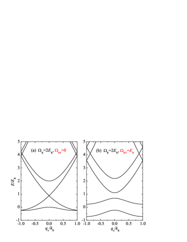
Figure 1: (color online) Energy band structure $E\left(q_{x}\right)$ in the absence (a) and presence (b) of spin-orbit lattice potential.

II.3 Band structure of spin-orbit coupled lattice

In Fig. 1, we present the band structure $E\left(q_{x}\right)$ of the spin-orbit coupled system at $\Omega_{RF}=0$ and $\Omega_{RF}=E_{R}$. In the absence of rf-coupling (Fig. 1a), the band structure is actually exactly identical to the single-particle dispersion Eq. (12). However, we have folded the entire dispersion into the first Brillouin zone $-k_{R}\leq q_{x}<k_{R}$. Thus, at the edge of Brillouin zone, $q_{x}=\pm k_{R}$, the band energy is at least two-fold degenerate. Moreover, some bands are also degenerate at $q_{x}=0$ due to the even-parity of the single-particle dispersion (12). In this case, for the wave function Eq. (19), there is only one non-zero (i.e., unity) coefficient in $a_{n+}$ or $a_{n-}$. With the rf-coupling (Fig. 1b), the degeneracy at the zone edge or at $q_{x}=0$ is lifted. We have a clear, well-resolved band structure. When the rf-coupling $\Omega_{RF}$ is large enough, a band gap also opens among the lowest three bands. Therefore, when the system is filled up to the top of the second band (i.e., the chemical potential $\mu<E_{R}$), a band insulator is formed.

III Radio-frequency spectroscopy in free space

Let us consider the rf-spectroscopy Chin2004 ; Schunck2008 , which is driven by a rf laser beam to transfer an atom in one of the two hyperfine states (say $\left|\downarrow\right\rangle$) to an empty hyperfine state $\left|3\right\rangle$. The state $\left|3\right\rangle$ is normally higher in energy by an amount of $\hbar\omega_{3\downarrow}$, due to the magnetic field splitting in bare atomic hyperfine levels. The Hamiltonian for the rf-transition may be written as,

$${\cal V}_{rf} = V_{0}\int d{\bf r}\left[\psi_{3}^{\dagger}\left({\bf r}\right)\psi_{\downarrow}\left({\bf r}\right)+\psi_{\downarrow}^{\dagger}\left({\bf r}\right)\psi_{3}\left({\bf r}\right)\right],$$ (27)

$$= V_{0}\int d{\bf r}\left[e^{-ik_{R}x}\psi_{3}^{\dagger}\left({\bf r}\right)\tilde{\psi}_{\downarrow}\left({\bf r}\right)+\text{H.c.}\right],$$ (28)

where $\psi_{3}^{\dagger}\left({\bf r}\right)$ is the field operator which creates an atom in $\left|3\right\rangle$ at the position ${\bf r}$ and $V_{0}$ is the strength of the rf drive. In the second line of the above equation, we have taken the gauge transformation for $\psi_{\downarrow}\left({\bf r}\right)$. As a result, there is an effective momentum transfer $k_{R}{\bf e}_{x}$.

The transfer strength of the rf-transition $\Gamma\left(\omega\right)$ can be calculated by using the Fermi’s golden rule:

$$\Gamma\left(\omega\right)=\sum_{i,f}\left|\left\langle\Phi_{f}\right|{\cal V}_{rf}\left|\Phi_{i}\right\rangle\right|^{2}f\left(E_{i}-\mu\right)\delta\left[\hbar\omega-\hbar\omega_{3\downarrow}-\left(E_{f}-E_{i}\right)\right].$$ (29)

Here, the summation is over all the possible initial states $\Phi_{i}$ (with energy $E_{i}$) and final states $\Phi_{f}$ (with energy $E_{f}$) and $f\left(E_{i}-\mu\right)$ is the Fermi distribution function. The Dirac delta function ensures energy conservation during transition. Hereafter, without any confusion we shall ignore the energy splitting in the bare atomic hyperfine levels and set $\omega_{3\downarrow}=0$. To calculate the overlap between the initial and final wave-functions $\left|\left\langle\Phi_{f}\right|{\cal V}_{rf}\left|\Phi_{i}\right\rangle\right|$, let us take the $l$-th band eigenstate $\Phi_{i}=\Phi^{(l)}\left(q_{x},{\bf k}_{\perp};{\bf r}\right)\equiv[\tilde{\psi}_{\uparrow}^{(l)}\left({\bf r}\right),\tilde{\psi}_{\downarrow}^{(l)}\left({\bf r}\right)]^{T}$ as the initial state, where

$$\tilde{\psi}_{\downarrow}^{(l)}\left({\bf r}\right)=\sum_{n=-\infty}^{+\infty}\left[a_{n+}^{(l)}\sin\theta_{{\bf k}_{n}}+a_{n-}^{(l)}\cos\theta_{{\bf k}_{n}}\right]e^{i\left(2nk_{R}+q_{x}\right)x}e^{i{\bf k}_{\perp}\cdot{\bf r}_{\perp}},$$ (30)

and $E_{i}=E^{(l)}(q_{x})+\hbar^{2}k_{\perp}^{2}/(2M)$. It is easy to see that, in order to have a nonzero overlap, the final state must be a plane wave, i.e., $e^{i({\bf k}_{n}-k_{R}{\bf e}_{x})\cdot{\bf r}}$, with which the overlap of wave functions is given by,

$$\left|\left\langle\Phi_{f}\right|{\cal V}_{rf}\left|\Phi_{i}\right\rangle\right|^{2}=\left[a_{n+}^{(l)}\sin\theta_{{\bf k}_{n}}+a_{n-}^{(l)}\cos\theta_{{\bf k}_{n}}\right]^{2},$$ (31)

and the final state energy is

$$E_{f}=\frac{\hbar^{2}k_{\perp}^{2}}{2M}+\frac{\hbar^{2}\left(k_{nx}-k_{R}\right)^{2}}{2M}.$$ (32)

By taking into account all the possibilities for $\Phi_{i}$ and $\Phi_{f}$, the transfer strength can then be written in the form,

$$\Gamma\left(\omega\right) = \int\limits_{0}^{\infty}\frac{k_{\perp}dk_{\perp}}{\left(2\pi\right)^{2}}\int\limits_{-k_{R}}^{+k_{R}}dq_{x}\sum_{l=0}^{\infty}\sum_{n=-\infty}^{+\infty}\left[a_{n+}^{(l)}\sin\theta_{{\bf k}_{n}}+a_{n-}^{(l)}\cos\theta_{{\bf k}_{n}}\right]^{2}$$ (33)

$$\times f\left[\frac{\hbar^{2}k_{\perp}^{2}}{2M}+E^{(l)}(q_{x})-\mu\right]\delta\left[\hbar\omega+E^{(l)}(q_{x})-\frac{\hbar^{2}\left(k_{nx}-k_{R}\right)^{2}}{2M}\right],$$

where $k_{nx}=2nk_{R}+q_{x}$ and $\theta_{{\bf k}_{n}}=\arctan[(\sqrt{h^{2}+\lambda^{2}k_{nx}^{2}}-\lambda k_{nx})/h]$. The integration over $k_{\perp}$ can be done analytically. We find that,

$$\int\limits_{0}^{\infty}\frac{k_{\perp}dk_{\perp}}{\left(2\pi\right)^{2}}f\left[\frac{\hbar^{2}k_{\perp}^{2}}{2M}+E^{(l)}(q_{x})-\mu\right]=\frac{Mk_{B}T}{4\pi^{2}\hbar^{2}}\ln\left\{1+\exp\left[-\frac{E^{(l)}(q_{x})-\mu}{k_{B}T}\right]\right\}.$$ (34)

Experimentally, the momentum of the transferred atom, $k_{nx}$, could be resolved exptMIT ; Stewart2008 . Therefore, we may define a momentum-resolved transfer strength ($k_{x}\equiv k_{nx}-k_{R}$),

$$\Gamma\left(k_{x},\omega\right)=\frac{Mk_{B}T}{4\pi^{2}\hbar^{2}}\sum_{l=0}^{\infty}\left[a_{n+}^{(l)}\sin\theta_{{\bf k}_{n}}+a_{n-}^{(l)}\cos\theta_{{\bf k}_{n}}\right]^{2}\ln\left\{1+\exp\left[-\frac{E^{(l)}(q_{x})-\mu}{k_{B}T}\right]\right\}\delta\left[\hbar\omega+E^{(l)}(q_{x})-\frac{\hbar^{2}k_{x}^{2}}{2M}\right],$$ (35)

where the quasi-momentum $q_{x}$ and the index $n$ are now determined from the momentum $k_{nx}=k_{x}+k_{R}$. The total transfer strength is simply $\Gamma(\omega)=\int\nolimits_{-\infty}^{+\infty}dk_{x}\Gamma(k_{x},\omega)$. To take into account the energy resolution of the spectroscopy $\gamma\sim 0.1E_{R}$ exptMIT , we may replace the Dirac delta function by, $\delta\left(x\right)=(\gamma/\pi)/[x^{2}+\gamma^{2}]$. To reveal more clearly the band structure, it is also useful to calculate

$$\tilde{\Gamma}\left(k_{nx},\tilde{\omega}\right)\equiv\Gamma\left(k_{x}+k_{R},\omega+\frac{\hbar k_{x}^{2}}{2M}\right),$$ (36)

for which, the Dirac delta function takes the form $\delta[\hbar\tilde{\omega}+E^{(l)}(q_{x})]$.

III.1 Momentum-resolved rf spectroscopy in free space

We are now ready to calculate the momentum-resolved rf spectroscopy of a uniform Fermi gas in the spin-orbit coupled lattice. For a given $k_{x}$, we obtain first the quasi-momentum $q_{x}$ and the index $n$, and then solve the energy bands $E^{(l)}(q_{x})$ and eigenstates $a_{n+}^{(l)}$ and $a_{n-}^{(l)}$. For the given chemical potential $\mu$ and temperature $k_{B}T$, which are in units of $E_{R}$, we finally take the summation over the band index $l$ and obtain the momentum-resolved transfer strength. Figs. 2a-2c and 2d-2f report the linear contour plot of rf spectroscopy in the absence ($\Omega_{RF}=0$) and presence ($\Omega_{RF}=E_{R}$) of lattice potential, respectively, with increasing the chemical potential $\mu$ at zero temperature. The transfer strength always becomes stronger with increasing $\mu$, since there are more and more atoms in the system.

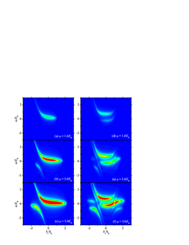
Figure 2: (color online) Momentum-resolved rf spectroscopy of a uniform Fermi gas without (left panel, $\Omega_{RF}=0$) or with (right panel, $\Omega_{RF}=E_{R}$) lattice potential at zero temperature. The Raman coupling strength is $\Omega_{R}=2E_{R}$. From (a) to (c), or from (d) to (f), we increase the chemical potential $\mu$ from $E_{R}$ to $5E_{R}$. Here the intensity of the contour plot increases linearly from $0$ (blue) to $0.1M/\hbar^{2}$ (red).

The spectroscopy is already very interesting without a lattice, as shown in Figs. 2a-2c. At a low chemical potential $\mu=E_{R}$, only the lower helicity branch of the single-particle dispersion Eq. (12) is occupied. The spin-orbit coupling leads to a long tail at negative momentum and high frequency, in sharp contrast to a single Dirac delta function $\delta(\omega)$ in the absence of spin-orbit coupling. As the chemical potential increases (Figs. 2b and 2c), the upper helicity branch gets occupied. In the spectroscopy, this creates a strong response at opposite momentum and frequency.

In the presence of a lattice potential induced by the rf-coupling, the spectroscopy is greatly modified by the formation of energy bands. At the chemical potential $\mu=E_{R}$ the lowest two bands, well-separated in energy, should already be occupied, as we can see from Fig. 1b. As a result, we observe in Fig. 2d the two different responses from the two bands. The energy gap between the first and second bands, which is at about $E_{R}$, is clearly resolved in the spectroscopy. With increasing the chemical potential, more and more energy bands come to contribute and the spectroscopy becomes more fragmented. There are some discontinuity at $k_{x}=\pm k_{R}$, indicating the existence of different energy gaps.

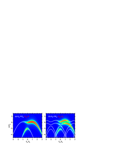
Figure 3: (color online) Linear contour plot of $\tilde{\Gamma}(k_{nx},\tilde{\omega})$ at $\Omega_{R}=2E_{R}$, $\mu=5E_{R}$, and $T=0$. The left plot and right plot correspond to the cases without and with lattice potential, respectively. The energy bands $-E^{(l)}(q_{x})$ are shown by thick white curves.

Fig. 3 shows $\tilde{\Gamma}(k_{nx},\tilde{\omega})$ at $\mu=5E_{R}$ with or without the lattice potential. As $\tilde{\Gamma}(k_{nx},\tilde{\omega})$ contains the Dirac delta function $\delta[\hbar\tilde{\omega}+E^{(l)}(q_{x})]$, we anticipate that the energy band $E^{(l)}(q_{x})$ can be seen clearly from the contour plot. Indeed, we find that the rf-response is peaked exactly at $-E^{(l)}(q_{x})$ (shown by white curves) within the experimental energy resolution. The strength of the response is determined by the coefficients $a_{n+}^{(l)}$ and $a_{n-}^{(l)}$. Therefore, by measuring momentum-resolved rf-spectroscopy $\Gamma\left(k_{x},\omega\right)$ and re-constructing $\tilde{\Gamma}(k_{nx},\tilde{\omega})$, we are able to obtain the complete information of the single-particle energy bands and eigenstates.

IV Radio-frequency spectroscopy in harmonic traps

We turn to address the realistic issue of harmonic traps, $V_{T}({\bf r})=M\omega_{0}^{2}r^{2}/2$, by using local density approximation. Within local density approximation, the whole system can be regarded as a collection of many uniform blocks with a local chemical potential $\mu-V_{T}({\bf r})$. The momentum-resolved rf spectroscopy is a sum of local spectroscopy over the whole trap,

$$\Gamma_{T}\left(k_{x},\omega\right)=\int d{\bf r}\Gamma\left[k_{x},\omega;\mu-V_{T}({\bf r})\right].$$ (37)

By substituting Eq. (35) for local spectroscopy and using the fact that

$$\int_{0}^{\infty}4\pi r^{2}dr\ln\left\{1+\exp\left[-\frac{E^{(l)}(q_{x})-\mu+V_{T}({\bf r})}{k_{B}T}\right]\right\}=-\left(\frac{2\pi k_{B}T}{M\omega_{0}^{2}}\right)^{3/2}\text{Li}_{5/2}\left(-\exp\left[-\frac{E^{(l)}(q_{x})-\mu}{k_{B}T}\right]\right),$$ (38)

we find that,

$$\Gamma_{T}\left(k_{x},\omega\right) = -\sqrt{\frac{E_{R}}{\pi}}\frac{\left(k_{B}T\right)^{5/2}}{\left(\hbar\omega_{0}\right)^{3}}\sum_{l=0}^{\infty}\left[a_{n+}^{(l)}\sin\theta_{{\bf k}_{n}}+a_{n-}^{(l)}\cos\theta_{{\bf k}_{n}}\right]^{2}$$ (39)

$$\times\text{Li}_{5/2}\left(-\exp\left[-\frac{E^{(l)}(q_{x})-\mu}{k_{B}T}\right]\right)\delta\left[\hbar\omega+E^{(l)}(q_{x})-\frac{\hbar^{2}k_{x}^{2}}{2M}\right].$$

Here Li${}_{n}(x)$ is the polylogarithm function. Experimentally, the trap frequency is about two order smaller than the recoil energy $E_{R}$. Hereafter, we shall take $\hbar\omega_{0}=0.01E_{R}$, according to the experimental setup at ShanXi University exptShanXi . In analogy to the uniform case, we may define

$$\tilde{\Gamma}_{T}\left(k_{nx},\tilde{\omega}\right)\equiv\Gamma_{T}\left(k_{x}+k_{R},\omega+\frac{\hbar k_{x}^{2}}{2M}\right),$$ (40)

in order to better visualize the energy band.

Figure 4: (color online) Comparison between momentum-resolved rf-spectroscopy in free space and in harmonic traps at zero temperature. Here, we take the same chemical potential $\mu=3E_{R}$ and use $\Omega_{R}=$ $\Omega_{RF}=2E_{R}$. The intensity of each contour plot increases from $0$ (blue) to its maximum value (red).

In Figs. 4a and 4b, we compare the momentum-resolved rf spectroscopy in free space and in harmonic traps, at $\Omega_{R}=$ $\Omega_{RF}=2E_{R}$ and at zero temperature. The chemical potential is taken the same value, i.e., $\mu=3E_{R}$. In each plot, we assign the red color to the maximum value of rf transfer strength. With traps, the rf-response from the higher bands is blurred by the trap average. However, the qualitative features of rf-spectroscopy remains the same, as we may anticipate. This strongly indicates that in harmonic traps we could still be able to re-construct the energy band structure by using momentum-resolved rf-spectroscopy.

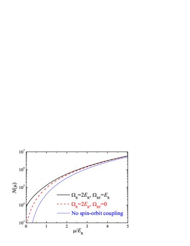
Figure 5: (color online) Total number of atoms as a function of chemical potential for a trapped Fermi gas. The cases with or without lattice potential are plotted by solid and dashed lines, respectively. For comparison, we show also the result without spin-orbit coupling by a thin solid line. Here, we take the trapping frequency $\hbar\omega_{0}=0.01E_{R}$.

To have a realistic estimate of the chemical potential in harmonic traps, it is useful to calculate the total number of atoms, which is given by $N=\int d{\bf r}n({\bf r})$, where the local density

$$n({\bf r})=\int\limits_{0}^{\infty}\frac{k_{\perp}dk_{\perp}}{\left(2\pi\right)^{2}}\int\limits_{-k_{R}}^{+k_{R}}dq_{x}\sum_{l=0}^{\infty}f\left[\frac{\hbar^{2}k_{\perp}^{2}}{2M}+E^{(l)}(q_{x})-\mu+V_{T}({\bf r})\right].$$ (41)

By integrating over $k_{\perp}$ and the spatial coordinates, we obtain,

$$N=-\sqrt{\frac{E_{R}}{\pi}}\frac{\left(k_{B}T\right)^{5/2}}{\left(\hbar\omega_{0}\right)^{3}}\int\limits_{-k_{R}}^{+k_{R}}dq_{x}\sum_{l=0}^{\infty}\text{Li}_{5/2}\left(-\exp\left[-\frac{E^{(l)}(q_{x})-\mu}{k_{B}T}\right]\right).$$ (42)

In Fig. 5, we plot the total number of atoms in harmonic traps as a function of chemical potential with or without the spin-orbit coupled lattice. For comparison, we show also the result for an ideal Fermi gas without any spin-orbit coupling, $N=\mu^{3}/[3(\hbar\omega_{0})^{3}]$. In the ShanXi experiment exptShanXi , the number of atoms is about $2\times 10^{6}$, corresponding to $\mu\sim 3E_{R}$.

IV.1 Momentum-resolved rf spectroscopy in harmonic traps

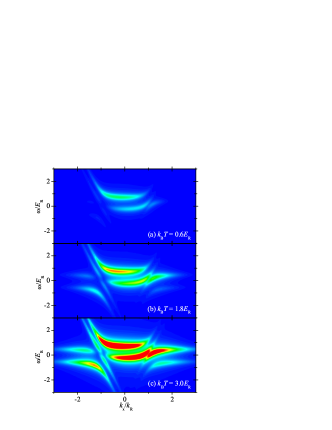
Figure 6: (color online) Temperature dependence of the momentum-resolved rf spectroscopy of a trapped atomic Fermi gas at $\Omega_{R}=2E_{R}$, $\Omega_{RF}=E_{R}$ and $\mu=3E_{R}$. The intensity of the contour plots increases from 0 (blue) to $2.5E_{R}^{3}/(\hbar\omega_{0})^{3}$ (red).

We examine first how the rf-spectroscopy is affected by temperature. In Fig. 6, we report the evolution of rf-spectroscopy with increasing temperature $k_{B}T$ from $0.2\mu$, $0.6\mu$ to $\mu$, where $\mu=3E_{R}$, $\Omega_{R}=2E_{R}$, and $\Omega_{RF}=E_{R}$. As the temperature increases, more and more energy bands are visible, as these bands become thermally occupied. Importantly, there is no significant thermal broadening for higher energy bands. They are all well-resolved even close to the degeneracy temperature $k_{B}T\sim\mu$. Note that, the typical temperature in the ShanXi experiment is about $0.6k_{B}T_{F}\sim 0.6\mu$.

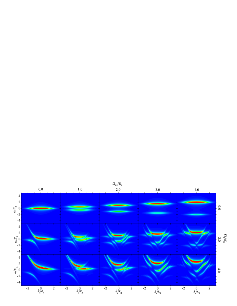
Figure 7: (color online) Evolution of the momentum-resolved rf spectroscopy of a trapped atomic Fermi gas as functions of the Raman and rf coupling strengths. Here, we take $\mu=3E_{R}$ and $k_{B}T=0.6\mu$. The intensity of the contour plots increases from 0 (blue) to $2E_{R}^{3}/(\hbar\omega_{0})^{3}$ (red).

We now explore the spin-orbit coupled system for a range of coupling strengths. In Fig. 7, we report the evolution of rf-spectroscopy as functions of the Raman coupling $\Omega_{R}$ and the rf coupling $\Omega_{RF}$, at $k_{B}T=0.6\mu$ and $\mu=3E_{R}$. This may be viewed as a realistic simulation of a future experiment for a non-interacting trapped Fermi gas of ⁴⁰K atoms in spin-orbit coupled lattice exptShanXi .

The reconstructed plot of $\tilde{\Gamma}_{T}(k_{nx},\tilde{\omega})$ is shown in Fig. 8, for a set of parameters $\Omega_{R}=\Omega_{RF}=2E_{R}$, $\mu=3E_{R}$, and $T=0.6\mu$. By comparing with the energy bands $-E^{(l)}(q_{x})$, which is plotted by thick white curves, it is readily seen that the band structure can be clearly extracted from a realistic momentum-resolved measurement at finite temperatures (i.e., $T\sim 0.6T_{F}$) and finite energy resolutions (i.e., $\gamma\sim 0.1E_{R}$).

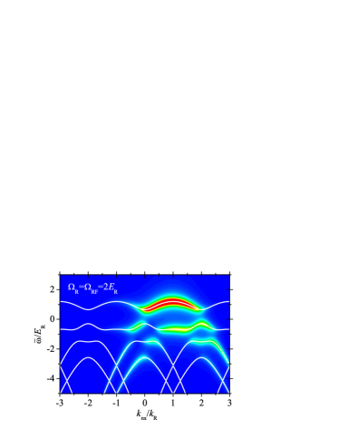
Figure 8: (color online) Linear contour plot of $\tilde{\Gamma}_{T}(k_{nx},\tilde{\omega})$ at $\Omega_{R}=\Omega_{RF}=2E_{R}$, $\mu=3E_{R}$, and $T=0.6\mu$. The energy bands $-E^{(l)}(q_{x})$ are shown by thick white curves. The intensity of the contour plots increases from 0 (blue) to $1.5E_{R}^{3}/(\hbar\omega_{0})^{3}$ (red).

V Conclusions

In summary, we have predicted theoretically momentum-resolved rf spectroscopy of a non-interacting atomic Fermi gas in a spin-orbit coupled lattice. We have shown that such a rf-spectroscopy, just like the angle-resolved photoemission spectroscopy in condensed matter physics ARPES , provides an ideal technique to characterize the non-trivial band structure of spin-orbit coupled lattice. Our predictions can be readily examined at ShanXi University by using ultracold ⁴⁰K atoms exptShanXi .

Using Feshbach resonances Chin2010 , a strongly interacting Fermi gas of ⁴⁰K atoms in spin-orbit coupled lattice would be created experimentally very soon. It is of great interest to study how the single-particle band structure is modified by strong interatomic interactions and fermionic superfluidity. In this case, we anticipate that momentum-resolved rf spectroscopy would provide very useful information.

References

• (1) Y.-J. Lin, R. L. Compton, K. JimΓ©nez-GarcΓ­a, J. V. Porto, and I. B. Spielman, Nature (London) 462, 628 (2009).
• (2) Y.-J. Lin, K. JimΓ©nez-GarcΓ­a, and I. B. Spielman, Nature (London) 471, 83 (2011).
• (3) R. A. Williams, L. J. LeBlanc, K. JimΓ©nez-GarcΓ­a, M. C. Beeler, A. R. Perry, W. D. Phillips, and I. B. Spielman, Science 335, 314 (2012).
• (4) K. JimΓ©nez-GarcΓ­a, L. J. LeBlanc, R. A. Williams, M. C. Beeler, A. R. Perry, and I. B. Spielman, Phys. Rev. Lett. 108, 225303 (2012).
• (5) S. Chen, J.-Y. Zhang, S.-C. Ji, Z. Chen, L. Zhang, Z.-D. Du, Y. Deng, H. Zhai, and J.-W. Pan, arXiv:1201.6018.
• (6) P. Wang, Z.-Q. Yu, Z. Fu, J. Miao, L. Huang, S. Chai, H. Zhai, and J. Zhang, arXiv:1204.1887.
• (7) L. W. Cheuk, A. T. Sommer, Z. Hadzibabic, T. Yefsah, W. S. Bakr, and M. W. Zwierlein, arXiv:1205.3483.
• (8) C. Wang, C. Gao, G.-M. Jian, and H. Zhai, Phys. Rev. Lett. 105, 160403 (2010).
• (9) C. Wu, I. Mondragon-Shem, and X.-F. Zhou, Chin. Phys. Lett. 28, 097102 (2011).
• (10) H. Hu, B. Ramachandhran, H. Pu, and X.-J. Liu, Phys. Rev. Lett. 108, 010402 (2012).
• (11) Y. Deng, J. Cheng, H. Jing, C.-P. Sun, and S. Yi, Phys. Rev. Lett. 108, 125301 (2012).
• (12) J. P. Vyasanakere, V. B. Shenoy, Phys. Rev. B 83, 094515 (2011).
• (13) Z. Q. Yu and H. Zhai, Phys. Rev. Lett. 107, 195305 (2011).
• (14) H. Hu, L. Jiang, X.-J. Liu, and H. Pu, Phys. Rev. Lett. 107, 195304 (2011).
• (15) M. Gong, S. Tewari, and C. Zhang, Phys. Rev. Lett. 107, 195303 (2011).
• (16) X.-J. Liu, L. Jiang, H. Pu, and H. Hu, Phys. Rev. A 85, 021603(R) (2012).
• (17) X.-L. Qi and S.-C. Zhang, Physics Today 63, 33 (2010).
• (18) M. Z. Hasan and C. L. Kane, Rev. Mod. Phys. 82, 3045 (2010).
• (19) C. Chin, M. Bartenstein, A. Altmeyer, S. Riedl, S. Jochim, J. Hecker Denschlag, and R. Grimm, Science 305, 1128 (2004).
• (20) C. H. Schunck, Y. Shin, A. Schirotzek, and W. Ketterle, Nature (London) 454, 739 (2008).
• (21) J. T. Stewart, J. P. Gaebler, D. S. Jin, Nature (London) 454, 744 (2008).
• (22) A. Damascelli, Z. Hussain, and Z.-X. Shen, Rev. Mod. Phys. 75, 473 (2003)
• (23) C. Chin, R. Grimm, P. S. Julienne, and E. Tiesinga, Rev. Mod. Phys. 82, 1225 (2010).