A quantum algorithm for solving some discrete mathematical problems by probing their energy spectra

Abstract

When a probe qubit is coupled to a quantum register that represents a physical system, the probe qubit will exhibit a dynamical response only when it is resonant with a transition in the system. Using this principle, we propose a quantum algorithm for solving discrete mathematical problems based on the circuit model. Our algorithm has favorable scaling properties in solving some discrete mathematical problems.

I Introduction

A lot of progress has been made in the field of quantum computation since the discovery of Shor’s factoring algorithm shor and Grover’s search algorithm grover . Quantum computing offers an increase in calculation speed for a number of problems childs ; nori . It has been suggested that for a fairly general class of quantum systems, especially discrete systems, an exponential increase in speed can be achieved using quantum simulators sl .

In Ref. farhi1 ; farhi2 , Farhi and coworkers developed a quantum adiabatic algorithm (QAA) for solving a discrete mathematical problem, the $3$-bit exact cover problem (EC$3$). In this algorithm, one starts from an initial Hamiltonian, $H_{B}$, and using its ground state as the initial state, and $H_{B}$ evolves to a final Hamiltonian $H_{P}$, whose ground state is the solution to the EC$3$ problem. The system evolves from the initial state to the ground state of $H_{P}$.

In this paper, we propose an alternative quantum algorithm for solving some discrete mathematical problems based on the circuit model. Our approach can be applied to any satisfiability problem in principle, here we demonstrate it with a particular instance of the exact cover problem, EC$3$.

The EC$3$ problem on a quantum computer can be formulated as follows farhi1 ; farhi2 : the $3$-bit instance of satisfiability is a Boolean formula with $M$ clauses

$$C_{1}\wedge C_{2}\wedge\cdots\wedge C_{M}\text{,}$$ (1)

where each clause $C_{l}$ is true or false depending on the values of a subset of the $n$ bits, and each clause contains three bits. The clause is true if and only if one of the three bits is $1$ and the other two are $0$. The task is to determine whether one (or more) of the $2^{n}$ assignments satisfies all of the clauses, that is, makes formula ($1$) true, and find the assignment(s) if it exists. Let $i_{C}$, $j_{C}$ and $k_{C}$ be the $3$ bits associated with clause C. For each clause C, we define an “energy” function

$$h_{C}(z_{i_{C}},z_{j_{C}},z_{k_{C}})\!=\!\Bigg{\{}\begin{array}[]{c}\!\!\!\!0,\,\,\mathrm{if}\,(z_{i_{C}},z_{j_{C}},z_{k_{C}})\ \mathrm{satisfies\ clause\ \emph{C}}\\ \!\!\!\hskip 0.02205pt1,\,\,\mathrm{if}\,(z_{i_{C}},z_{j_{C}},z_{k_{C}})\ \mathrm{violates\ clause\ \emph{C}}\end{array}$$ (2)

Then

$$H_{P,C}|z_{1}z_{2}\cdots z_{n}\rangle=h_{C}\left(z_{i_{C}},z_{j_{C}},z_{k_{C}}\right)|z_{1}z_{2}\cdots z_{n}\rangle,$$ (3)

where $|z_{j}\rangle$ is the $j$-th bit and has a value $0$ or $1$. Define

$$H_{P}=\sum_{C}H_{P,C}.$$ (4)

$H_{P}|\psi\rangle=0$, if and only if $|\psi\rangle$ is a state of the form $|z_{1}z_{2}\cdots z_{n}\rangle$, where the bit string $z_{1}z_{2}\cdots z_{n}$ satisfies all of the clauses, or a superposition of such states. If formula ($1$) has no satisfying assignments, the ground state (or states) of $H_{P}$ corresponds to the assignment (or assignments) that violates the fewest clauses. The computational basis of $|z_{1}z_{2}\cdots z_{n}\rangle$ is of dimension $N=2^{n}$.

II The algorithm

Our algorithm for solving the EC$3$ problem is described below.

First, we construct a Hamiltonian $\widetilde{H}$ with the form:

$$\widetilde{H}=\left(\begin{array}[]{cc}-I_{N}&0\\ 0&H_{P}\end{array}\right),$$ (5)

where $I_{N}$ is the $N$-dimensional identity operator, and $\widetilde{H}$ acts on the state space of a ($n+1$)-qubit quantum register $R_{S}$, which contains one ancilla qubit and $n$ qubits that represents the system. Then we let a probe qubit couple to $R_{S}$, and design a Hamiltonian $H$ for the whole system of the form

$$H=\frac{1}{2}\omega\sigma_{z}\otimes I_{2}^{\otimes\left(n+1\right)}+I_{2}\otimes\widetilde{H}+c\sigma_{x}\otimes A,$$ (6)

where $I_{2}$ is the two-dimensional identity operator. In Eq. ($6$), the first term is the Hamiltonian of the probe qubit, the second term is the Hamiltonian of the quantum register $R_{S}$, and the third term describes the interaction between the probe qubit and $R_{S}$. Here, $\omega$ is the frequency of the probe qubit ($\hbar=1$), and $c$ is the coupling strength between the probe qubit and $R_{S}$, whereas $\sigma_{x}$ and $\sigma_{z}$ are Pauli matrices. The operator $A$ acts on the state space of $\widetilde{H}$ and plays the role of an excitation operator. This operator contains $N$ terms, which provide all possible terms that excite the system from the subspace of $-I_{N}$ to the subspace of $H_{P}$,

$$A=\frac{1}{\sqrt{N}}(A_{1}+A_{2}+\cdots+A_{N}),$$ (7)

where

$$A_{1} = \sigma_{x}\otimes I_{2}\otimes I_{2}\otimes\cdots\otimes I_{2},$$

$$A_{2} = \sigma_{x}\otimes I_{2}\otimes\cdots\otimes I_{2}\otimes\sigma_{x},$$

$$\cdots,$$

$$A_{n+1} = \sigma_{x}\otimes\sigma_{x}\otimes I_{2}\otimes I_{2}\otimes\cdots\otimes I_{2},$$

$$A_{n+2} = \sigma_{x}\otimes I_{2}\otimes\cdots\otimes I_{2}\otimes\sigma_{x}\otimes\sigma_{x},$$

$$A_{n+3} = \sigma_{x}\otimes I_{2}\otimes\cdots\otimes\sigma_{x}\otimes I_{2}\otimes\sigma_{x},$$

$$\cdots,$$

$$A_{N} = \sigma_{x}\otimes\sigma_{x}\otimes\cdots\otimes\sigma_{x}\otimes\sigma_{x}.$$ (8)

Although the operator $A$ has an exponentially large number of terms, it can be implemented at a polynomial cost as

$$A=\sigma_{x}\otimes\left[\frac{1}{\sqrt{2}}(I_{2}+\sigma_{x})\right]^{\otimes n}.$$ (9)

We prepare $R_{S}$ in state

$$|\Psi_{0}\rangle=\frac{1}{\sqrt{N}}\sum_{j=1}^{N}|\varphi_{j}\rangle=\frac{1}{\sqrt{N}}\sum_{j=1}^{N}|0\rangle\otimes|j-1\rangle,$$ (10)

as the reference state, where $|\varphi_{j}\rangle=$ $|0\rangle\otimes|j-1\rangle$ and $|j-1\rangle$ are the states of the computational basis in the subspace of $I_{N}$, and $|0\rangle=\left(\begin{array}[]{c}1\\ 0\end{array}\right)$. This is achieved by initializing $R_{S}$ in state $|0\rangle^{\otimes\left(n+1\right)}$ and applying the operator $I_{2}\otimes H_{d}^{\otimes n}$, where $H_{d}$ is the Hadamard gate. The states $|\varphi_{j}\rangle$ are all eigenstates of $\widetilde{H}$ with eigenvalues of $-1$. Therefore, the reference state $|\Psi_{0}\rangle$ is also an eigenstate of $\widetilde{H}$ with eigenvalue $E_{0}=-1$. We set the frequency of the probe qubit $\omega=1$ and run the circuit in Fig. $1$. We repeat this procedure many times until the probe qubit decays to its ground state.

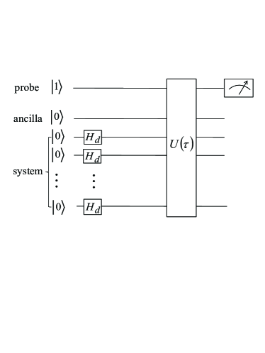
Figure 1: Quantum circuit for solving the exact cover problem EC$3$. $(n+2)$ qubits are required to solve an $n$-bit EC$3$ problem. The first line represents a probe qubit, and the next $n+1$ lines represent the quantum register $R_{S}$. $H_{d}$ represents the Hadamard gate, and $U(\tau)$ is the time evolution operator for the Hamiltonian given in Eq. ($6$).

The algorithm procedure is summarized as follows: $\left(i\right)$ prepare the first qubit in state $|1\rangle$ and the next ($n+1$)-qubit quantum register $R_{S}$ in state $|0\rangle^{\otimes\left(n+1\right)}$; $\left(ii\right)$ apply operator $I_{2}\otimes H_{d}^{\otimes n}$ on $R_{S}$, therefore $R_{S}$ is transformed into state $|\Psi_{0}\rangle$ as shown in Eq. ($10$); $\left(iii\right)$ implement the time evolution operator $U(\tau)=\exp\left(-iH\tau\right)$ where $H$ is given in Eq. ($6$); $\left(iv\right)$ read out the state of the probe qubit; $\left(v\right)$ repeat steps $\left(i\right)$ – $\left(iv\right)$ until a decay of the probe qubit to its ground state is observed. The quantum circuit for steps $\left(i\right)$ – $\left(iv\right)$ is shown in Fig. $1$.

III Efficiency of the algorithm

In our algorithm, $(n+2)$ qubits are required for solving an $n$-bit EC$3$ problem on a quantum computer, which increases linearly with the size of the problem. In the following paragraphs, we discuss the efficiency of the algorithm.

The efficiency of the algorithm is defined as the number of times that the circuit in Fig. $1$ must be run to observe a decay of the probe qubit. The number of times that the circuit must be run must be at least proportional to $1/P_{\text{decay}}$. The decay probability of a probe qubit that coupled to a system has been discussed in Ref. wan . In our case, we prepare $R_{S}$ in state $|\Psi_{0}\rangle$ and only consider the excitation from the subspace of $-I_{N}$ to the subspace of $H_{P}$. Therefore the decay probability of the probe qubit becomes:

$$P_{\text{decay}}=\sin^{2}\left(\frac{\Omega_{0j}\tau}{2}\right)\frac{Q_{0j}^{2}}{Q_{0j}^{2}+\left(E_{j}-E_{0}-\omega\right)^{2}},$$ (11)

where

$$Q_{0j}=2c|\langle\Psi_{j}|A|\Psi_{0}\rangle|,$$ (12)

and

$$\Omega_{0j}=\sqrt{Q_{0j}^{2}+\left(E_{j}-E_{0}-\omega\right)^{2}},$$ (13)

$|\Psi_{j}\rangle$ ($j=1,2,\ldots,N$) is the $j$-th energy eigenstate and $E_{j}$ is the corresponding eigenenergy of $H_{P}$, and according to Eq. ($4$), $E_{j}$ are discrete integers. Eq. ($11$) describes Rabi-oscillation dynamics, in which the quantum register $R_{S}$ and the probe qubit exchange an excitation; $R_{S}$ is excited from state $|\Psi_{0}\rangle$ to state $|\Psi_{j}\rangle$.

If a solution to the EC$3$ problem exists, the excitation frequency between the reference state $|\Psi_{0}\rangle$ and the state $|\Psi_{1}\rangle$ with eigenvalue $E_{1}=0$, which contains all solutions to the problem, is $1$. With the probe qubit frequency being set to $\omega=1$ and assuming there exists a solution to the problem, the decay probability of the probe qubit becomes

$$P_{\text{decay}}=\sin^{2}\left(\frac{Q_{01}\tau}{2}\right),$$ (14)

where

$$Q_{01} = 2c|\langle\Psi_{1}|A|\Psi_{0}\rangle|$$ (15)

$$= 2c\sum_{j=1}^{N}\sum_{i=1}^{m}\frac{1}{\sqrt{Nm}}|\langle 1|\langle\mu_{i}|A|\varphi_{j}\rangle|$$

$$= 2cNm\frac{1}{\sqrt{Nm}}\frac{1}{\sqrt{N}}$$

$$= 2c\sqrt{m}.$$

This term describes the summation over all excitation channels in the Rabi-oscillation. Here, $|\Psi_{1}\rangle=\sum_{i=1}^{m}|1\rangle|\mu_{i}\rangle/\sqrt{m}$ encodes all solutions to the EC$3$ problem, which is a superposition of all $m$ assignments that satisfy all of the clauses. In addition, $|\mu_{i}\rangle$ are these assignments, which are the basis states of $H_{P}$ with eigenvalues $0$ and degeneracy $m$. Here, although $1/\sqrt{N}$ appears in both the operator $A$ and the reference state $|\Psi_{0}\rangle$, there are $N$ terms in the excitation operator $A$, which provide $N$ excitation channels. For each state $|\mu_{i}\rangle$, there are $N$ excitation channels connecting it to the reference state $|\Psi_{0}\rangle$. Considering the degeneracy of the states $|\mu_{i}\rangle$,these channels contribute a factor of $Nm$ to the whole term. From Eq. ($15$), we can see that as $m$ increases, there are more excitation channels, and the period of $P_{\text{decay}}$ decreases. By knowing $Q_{01}$, we can choose a specific evolution time $\tau$ considering the degeneracy of the ground state of the problem, such that the probe qubit has a high decay probability and therefore the algorithm has a high efficiency. By attempting to guess $m$, one can quickly identify the optimal evolution time $\tau$ for implementing the algorithm.

From Eq. ($14$) and Eq. ($15$) above, we can see that the decay probability, and therefore the efficiency of the algorithm, depends on the coupling strength $c$ and the evolution time $\tau$. In general, we need to set $c$ to be small so that we have weak system-probe coupling. The evolution time $\tau$ should be large, such that the change of the system is clear and one obtains a high decay probability.

When we set $\omega=1$, the coupling between the reference state and all other states, except the state with an eigenvalue equal to zero, also contributes to the decay probability of the probe qubit, and therefore introduces an error in $P_{\text{decay}}$. We now evaluate this error, $P_{\text{decay}}^{\text{err}}$.

$$P_{\text{decay}}^{\text{err}} = \sum_{j=2}^{N}\sin^{2}\left(\frac{\Omega_{0j}\tau}{2}\right)\frac{Q_{0j}^{2}}{Q_{0j}^{2}+\left(E_{j}-E_{0}-\omega\right)^{2}}$$ (16)

$$< \sum_{j=2}^{N}\frac{Q_{0j}^{2}}{E_{j}{}^{2}}$$

$$\leq \sum_{j^{\prime}=2}^{N_{m}}\frac{4c^{2}m_{j}}{\left(j^{\prime}-1\right)^{2}}$$

$$< 4c^{2}m_{0}\frac{\pi^{2}}{6}=\frac{2}{3}m_{0}\pi^{2}c^{2},$$

where $E_{0}=-1$ is the eigenvalue of the reference state and $m_{j}$ represents the degeneracy of the assignments with eigenvalue $E_{j}$. $N_{m}$ is the eigenenergy of the highest energy level of the problem, and as $N_{m}\rightarrow\infty$, $\sum_{j^{\prime}=2}^{N_{m}}\frac{1}{\left(j^{\prime}-1\right)^{2}}=\frac{\pi^{2}}{6}$. $m_{0}$ is the maximum of $m_{j}$. When there is no energy level with exponentially large degeneracy, the term $2m_{0}\pi^{2}c^{2}/3$ can be small because $c$ can be set small, but not exponentially small. We can then constrain this error to be very small. In this case, the algorithm can be completed in a finite time $\tau$.

IV Implementation of the algorithm

We now discuss the implementation of the algorithm. In the algorithm, we must implement the time evolution operator $U(\tau)=\exp\left(-iH\tau\right)$. In the Hamiltonian $H$, as shown in Eq. ($6$), the first two terms commute with each other, while they do not commute with the third term. The operator $U(\tau)$ can be implemented using the procedure of quantum simulation based on the Trotter-Suzuki formula nc :

$$U(\tau)\!=\!\left[e^{-i\left(\frac{1}{2}\omega\sigma_{z}+\widetilde{H}\right)\tau/L}e^{-i\left(c\sigma_{x}\otimes A\right)\tau/L}\right]^{L}\!+\!O\!\left(\frac{1}{L}\right),$$ (17)

where $L$ does not depend on the size of the problem. $L$ can be made sufficiently large such that the error is bounded by some threshold sl .

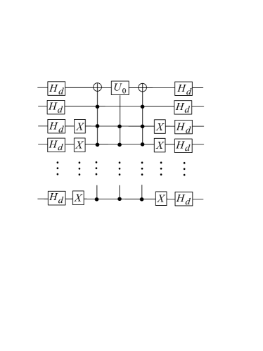
Figure 2: Quantum circuit for implementing the unitary operator $e^{-i(c\sigma_{x}\otimes A)\tau/L}$, where operator $A$ is given in Eq. ($9$). $H_{d}$ is the Hadamard gate and $U_{0}=e^{i\sqrt{2^{n}}c\tau/L\sigma_{z}}$, where $\sigma_{z}$ are the Pauli matrices.

In Eq. ($17$), the unitary operator $e^{-i\left(\frac{1}{2}\omega\sigma_{z}+\widetilde{H}\right)\tau/L}$ is diagonal and can be efficiently implemented. For the unitary operator $e^{-i\left(c\sigma_{x}\otimes A\right)\tau/L}$, the Hamiltonian $c\sigma_{x}\otimes A$ involves a many-body interaction. In Ref. bravyi , it was shown that a many-body interaction Hamiltonian can be efficiently simulated by a Hamiltonian with two-body interactions. The unitary operator $e^{-i(c\sigma_{x}\otimes A)\tau/L}$ can be implemented using the circuit shown in Fig. $2$. In the circuit, the $\left(n+1\right)$ and $n$-qubit controlled unitary operators can be efficiently implemented with $O\left(n^{2}\right)$ elementary gates barenco .

The second term in the Hamiltonian $H$, $\widetilde{H}$, as shown in Eq. ($5$), can be seen as a controlled-$H_{P}$ (C-$H_{P}$) operation. The operation that calculates $H_{P}$ can be taken as an oracle. In our algorithm, this oracle is entangled with the probe qubit. The number of times that the C-$H_{P}$ oracle is implemented is $L$. Therefore, the implementation of $U(\tau)$ scales polynomially with the size of the problem.

V Example: solving an $8$-bit EC$3$ problem

In the following, we present an example to demonstrate an application of the algorithm.

Considering an $8$-bit EC$3$ problem, we chose three cases of the $3$-bit sets of clauses, which have one, two, and four satisfying assignments for the problem, respectively. As discussed above, $10$ qubits are required to solve this problem using our algorithm. We set the coupling coefficient $c=0.002$ and run the algorithm for different evolution times $\tau$. As the probe qubit decays to the state $|0\rangle$, the state of the last $8$ qubits of the quantum register $R_{S}$ encodes all of the solutions to the above EC$3$ problem. Case $i)$: the $3$-bit sets are {$1,2,8$}, {$2,3,6$}, {$2,3,7$}, {$2,4,5$}, {$2,5,6$}, and {$3,5,8$}. The solution to the $8$-bit EC$3$ problem for this case is $|00010111\rangle$. Case $ii)$: the $3$-bit sets are chosen to be {$1,4,5$}, {$1,7,8$}, {$2,4,8$}, {$2,7,8$}, {$4,5,8$}, and {$5,6,7$}. The solution to the problem for this case is $|00010010\rangle$ and $|00110010\rangle$. Case $iii)$: the $3$-bit sets are {$1,3,5$}, {$1,6,8$}, {$2,4,6$}, {$2,6,8$}, and {$4,5,7$}. The solution to the problem for this case is $|00001100\rangle$, $|00100110\rangle$, $|00110001\rangle$, and $|11000010\rangle$.

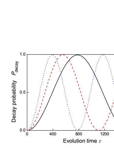
Figure 3: (Color online) Decay probability of the probe qubit vs. evolution time $\tau$. The frequency of the probe qubit $\omega=1$ and the coupling strength $c=0.002$. The black solid line shows the result for case $i$): the $3$-bit sets are {$1,2,8$}, {$2,3,6$}, {$2,3,7$}, {$2,4,5$}, {$2,5,6$}, and {$3,5,8$}; the red dashed line shows the result for case $ii$): the $3$-bit sets are {$1,4,5$}, {$1,7,8$}, {$2,4,8$}, {$2,7,8$}, {$4,5,8$}, and {$5,6,7$}; and the blue dotted line shows the result for case $iii$): the $3$-bit sets are {$1,3,5$}, {$1,6,8$}, {$2,4,6$}, {$2,6,8$}, and {$4,5,7$}. The simulated results fit exactly with the analytical results predicted in Eq. ($14$). Atomic units are used in the figure.

In Fig. $3$, we show the variation of simulated $P_{\text{decay}}$ with the evolution time $\tau$ for the above three cases. The black solid line, the red dashed line, and the blue dotted line show the results for cases $i)$, $ii)$ and $iii)$, respectively. In the above three cases, the decay probability almost reaches unity at $\tau=800$, $\tau=550$, and $\tau=400$, respectively. This result shows that the algorithm can be run efficiently. From the figure we can also see that as the number of satisfying assignments increases, the period of $P_{\text{decay}}$ decreases. The simulated $P_{\text{decay}}$ fits exactly with the analytical results predicted by Eq. ($14$). In the case in which there is no solution to the problem, if we still set the probe qubit frequency $\omega=1$, then $P_{\text{decay}}$ approaches zero.

VI Discussion

We have developed a quantum algorithm for solving a specific discrete mathematical problem, the EC$3$ problem. In our algorithm for solving the EC$3$ problem, we construct a Hamiltonian that contains the Hamiltonian of the problem and a Hamiltonian with the same dimension $N$ as the problem, whose eigenstates have degeneracy $N$ and eigenvalues (in our case, $-1$) lower than the smallest eigenvalue of the problem. The second Hamiltonian is used as a reference point. If a solution to the problem exists, we will observe the decay of the probe qubit at the excitation frequency (in our case, $1$) between the reference state and the eigenstates with an eigenvalue of zero. In this case, the system register evolves to its ground state, which is a superposition state that encodes the solution to the EC$3$ problem. If there is no solution to the problem, we can increase the frequency of the probe qubit discretely (because the energy function of the problem is discrete). The first frequency at which the probe qubit decays indicates the ground state of the system which encodes the assignment that violates the smallest number of clauses.

In our algorithm, one can determine whether there exists a solution to the problem immediately by performing a measurement on the probe qubit. If the probe qubit decays to its ground state, it indicates that a solution to the problem exists, otherwise the problem has no solution. The last $n$ qubits of the register $R_{S}$ encodes the solution to the problem if one observes a decay of the probe qubit. The solution can be in a superposition state of the multiple bit strings that satisfy the Boolean formula. And these bit strings can be obtained by employing the quantum state tomography.

Our algorithm can be applied to a large number of discrete mathematical problems, such as some combinatorial optimization problems. The procedure is similar: map the discrete mathematical problem on a quantum computer, therefore the problem is transferred to looking for the eigenstates with the lowest eigenenergy of the quantum system; Construct a $(n+1)$-qubit quantum register, which contains one ancilla qubit and $n$ qubits that represents the system. Then couple this quantum register with a probe qubit, which is used for probing the energy spectra of the system. And the whole system is driven by the Hamiltonian as shown in Eq. ($6$). By varying the frequency of the probe qubit discretely, the ground state or any desired eigenstates of the system can be found, which in general, encodes the information of the solution to the problem.

- (1) P. W. Shor, in Proceedings of the Symposium on the Foundations of Computer Science, 1994, Los Alamitos, California (IEEE Computer Society Press, New York, 1994), pp. 124 C134.
- (2) L. K. Grover, Phys. Rev. Lett. 79, 325 (1997).
- (3) A. M. Childs, W. van Dam, Rev. Mod. Phys. 82(1), 1 (2010).
- (4) I. Buluta, F. Nori, Science 326, 108 (2009).
- (5) S. Lloyd, Science 273, 1073 (1996).
- (6) E. Farhi, J. Goldstone, S. Gutmann, e-print quant-ph/0007071v1 (2000)
- (7) E. Farhi, J. Goldstone, S. Gutmann, J. Lapan, A. Lundgren, D. Preda, Science 292, 472 (2001).
- (8) H. Wang, S. Ashhab, F. Nori, Phys. Rev. A 85, 062304 (2012).
- (9) M. A. Nielsen, I. L. Chuang, Quantum computation and quantum information. (Cambridge Univ. Press, Cambridge, England, 2000).
- (10) S. Bravyi, D. P. DiVincenzo, D. Loss, B. M. Terhal, Phys. Rev. Lett. 101, 070503 (2008).
- (11) A. Barenco, et al. Phys. Rev. A 52, 3457 (1995).