Revealing The Millimeter Environment of the New FU Orionis Candidate HBC722 with the Submillimeter Array

Abstract

We present 230 GHz Submillimeter Array continuum and molecular line observations of the newly discovered FUor candidate HBC722. We report the detection of seven 1.3 mm continuum sources in the vicinity of HBC722, none of which correspond to HBC722 itself. We compile infrared and submillimeter continuum photometry of each source from previous studies and conclude that three are Class 0 embedded protostars, one is a Class I embedded protostar, one is a Class I/II transition object, and two are either starless cores or very young, very low luminosity protostars or first hydrostatic cores. We detect a northwest-southeast outflow, consistent with the previous detection of such an outflow in low-resolution, single-dish observations, and note that its axis may be precessing. We show that this outflow is centered on and driven by one of the nearby Class 0 sources rather than HBC722, and find no conclusive evidence that HBC722 itself is driving an outflow. The non-detection of HBC722 in the 1.3 mm continuum observations suggests an upper limit of 0.02 M_⊙ for the mass of the circumstellar disk. This limit is consistent with typical T Tauri disks and with a disk that provides sufficient mass to power the burst.

1. Introduction

FU Orionis objects (hereafter FUors) are a group of young, pre-main sequence stars observed to flare in brightness by $4-6$ magnitudes in the optical and remain bright for decades (Herbig 1977). They are named after the prototype FU Orionis, which flared by about 6 magnitudes in 1936 and has remained in an elevated state to the present day (Wachmann 1954; Herbig 1966). Only 10 confirmed FUors are known to exist from direct observations of flares, with about another 10 identified based on similar spectral characteristics to the confirmed FUors (see Reipurth & Aspin 2010 for a recent review). The large amplitude flares are attributed to enhanced accretion from the surrounding circumstellar disk (Hartmann & Kenyon 1985), with the accretion rate from the disk onto the star increasing to up to $\sim 10^{-4}$ M_⊙ yr^-1 (Hartmann & Kenyon 1996). Various triggering mechanisms for the accretion bursts have been proposed, including interactions with binary companions (Bonnell & Bastien 1992), thermal instabilities (Hartmann & Kenyon 1996), and gravitational and magnetorotational instabilities (Zhu et al. 2007, 2009a, 2009b; Vorobyov & Basu 2010). FUors are especially interesting and relevant to general star formation studies because they may represent the late, optically visible end stages of episodic accretion bursts and luminosity flares through the duration of the embedded phase (e.g., Kenyon et al. 1990; Enoch et al. 2009; Evans et al. 2009; Vorobyov 2009; Dunham et al. 2010; Dunham & Vorobyov 2012). With so few bona-fide FUors, detailed observations of each one are necessary in order to characterize their properties and understand their place in the general star formation process.

In this paper, we present 230 GHz Submillimeter Array (SMA; Ho et al. 2004) observations of the newly discovered FUor candidate HBC722. As described in more detail in §2 below, HBC722 is located within a small group of $\sim$ 10 young stars, greatly complicating the analysis of existing, low-resolution single-dish ground and space-based (sub)millimeter data. The SMA 230 GHz continuum and molecular line observations presented in this paper are motivated by a need to disentagle the millimeter emission from the various sources in the vicinity of HBC722 in order to better determine its evolutionary status and physical properties. The organization of this paper is as follows: a brief summary of HBC722 is given in §2, a description of the observations and data reduction is provided in §3, the basic results are presented in §4, including the continuum data in §4.1 and the CO line data in §4.2, a discussion of the detected continuum sources is presented in §5.1, a discussion of the evolutionary status of HBC722 is given in 5.2, and a summary of our results is presented in §6.

2. HBC722

HBC722, also known as V2493 Cyg, LkH$\alpha$ 188-G4, and PTF10qpf, is located at R.A. = 20:58:17.03, decl. = $+$43:53:43.4 (J2000) in the “Gulf of Mexico” region of the North American/Pelican Nebula Complex at a distance of 520 pc (Straizys et al. 1989; Laugalys et al. 2006). Prior to 2010 it was regarded as an emission-line star with a spectral type of K7$-$M0 and $A_{\rm V}$ of 3.4 magnitudes (Cohen & Kuhi 1979). Semkov et al. (2010) and Miller et al. (2011) independently reported a $4-5$ magnitude optical flare in HBC722. This flare began sometime before 2010 May, reached peak brightness in late 2010 September, followed a similar rise in brightness as other FUors, and exhibited spectral characteristics indicative of FUors (Semkov & Peneva 2010a; Semkov & Peneva 2010b; Semkov et al. 2010; Munari et al. 2010; Leoni et al. 2010; Miller et al. 2011). Prior to the flare, HBC722 featured a spectral energy distribution (SED) consistent with a Class II T Tauri star, with $L_{bol}$ $=0.85$ L_⊙ and infrared spectral slope $\alpha=-0.77$ (Kóspál et al. 2011; Miller et al. 2011). During the flare $L_{bol}$ increased to $8.7-12$ L_⊙. After the peak brightness was reached in late 2010 September, HBC722 entered a phase of rapid decline, decreasing by $\sim 0.5$ magnitudes in the optical by 2010 December (Kóspál et al. 2011). Based on a linear extrapolation of this initial decline, Kóspál et al. (2011) predicted a return to quiescence by late 2011 or early 2012, much too quickly to be a FUor. They also noted that the outburst $L_{bol}$ and mass accretion rate implied by this $L_{bol}$ are on the low end for FUors. However, unpublished photometry from the American Association of Variable Star Observers (AAVSO) shows that the optical brightness of HBC722 stopped its decline in early 2011, remained constant throughout most of 2011 at $3-4$ magnitudes above the quiescent brightness, and increased by about $0.5-1$ magnitudes between 2011 September and 2012 June. The cessation in early 2011 of the initial rapid decline has been very recently confirmed by Lorenzetti et al. (2012) and Semkov et al. (2012).

HBC722 was imaged by the Spitzer Space Telescope (Werner et al. 2004) at $3.6-8$ $\mu$m with the Infrared Array Camera (IRAC; Fazio et al. 2004) and $24-160$ $\mu$m with the Multiband Imaging Photometer for Spitzer (MIPS; Rieke et al. 2004) as part of a large survey of the North American and Pelican Nebula Complex (Guieu et al. 2009; Rebull et al. 2011). HBC722 is located within a small group of $\sim$ 10 young stars called the LkH$\alpha$ group by Cohen & Kuhi (1979), all located within approximately $20-30$″ ($10400-15600$ AU at the assumed distance of 520 pc) of HBC722. Several are detected in the mid-infrared with Spitzer and are thus still associated with dust in surrounding disks and envelopes, emphasizing the complex nature of this region (see Figure 1 of Green et al. [2011] and §5.1 below).

Green et al. (2011) presented (sub)millimeter data on HBC722 and its surrounding region observed with the Herschel Space Observatory (Pilbratt et al. 2011) and Caltech Submillimeter Observatory (CSO), including Herschel $70-500$ $\mu$m images with $5-36$″ resolution, Herschel $50-600$ $\mu$m full spectral scans, a 350 $\mu$m image with 9″ resolution obtained with the Submillimeter High Angular Resolution Camera II (SHARC-II) at the CSO, and a ¹²CO J $=2-1$ map with 30″ resolution obtained at the CSO. HBC722 is detected at 70 $\mu$m with Herschel; at all longer wavelengths the resolution is insufficient to resolve HBC722 from other, nearby sources. Green et al. noted that the $100-500$ $\mu$m Herschel emission does not peak on HBC722, suggesting it is not the dominant source of submillimeter emission. No emission is detected at the position of HBC722 in higher-resolution 350 $\mu$m SHARC-II data, suggesting that this source is no longer associated with a circumstellar envelope, consistent with the pre-outburst classification as a Class II T Tauri star. The 30″ resolution ¹²CO J $=2-1$ map presented by Green et al. clearly shows a NW-SE outflow centered near HBC722 (see their Figure 2 and §4.2 below), but the resolution is insufficient to definitively identify the driving source. In this paper, we present high angular resolution 1.3 mm continuum and ¹²CO J $=2-1$ observations obtained with the SMA in order to identify which sources in the vicinity of HBC722 are associated with (sub)millimeter continuum emission, characterize each source, and identify the driving source(s) of the outflow(s) in this region.

3. Observations and Data Reduction

One track of observations of HBC722 was obtained with the SMA on 20 May 2011 in the compact configuration with seven antennas, providing projected baselines ranging from 5 to 76 m. A two pointing mosaic was adopted to fully map the multiple sources in the vicinity of HBC722 (see, e.g., Figure 1 of Green et al. [2011]). The phase centers of the two pointings are R.A.=20:58:16.56, decl.=$+$43:53:52.9 (J2000) and R.A.=20:58:17.67, decl.=$+$43:53:31.0 (J2000), with the total observing time divided equally between the two pointings. The observations were obtained with the 230 GHz receiver and included 4 GHz of bandwidth per sideband, with 12 GHz spacing between the centers of the two sidebands. The correlator was configured such that the lower sideband (LSB) covered approximately $216.8-220.8$ GHz while the upper sideband (USB) covered aproximately $228.8-232.8$ GHz, providing simultaneous observations of the ¹²CO, ¹³CO, C¹⁸O J $=2-1$, N₂D⁺ J $=3-2$, and SiO J $=5-4$ lines. The lines were observed with either 256 (¹³CO, SiO) or 512 (¹²CO, C¹⁸O, N₂D⁺) channels in the 104 MHz bands, providing channel separations of 0.53 and 0.26 km s^-1, respectively. The remaining bands were used to measure the 1.3 mm continuum with a total bandwidth of 5.49 GHz.

The observations were obtained in moderate weather conditions, with the zenith opacity at 225 GHz ranging between $0.2-0.25$ and the system temperature typically $\sim$ 250 K, ranging between $150-400$ K depending on elevation. Regular observations of the sources MWC349a and BLLAC were interspersed with those of HBC722 for gain calibration. Saturn and 3C279 were used for passband calibration, and Uranus was used for absolute flux calibration. We estimate a 20% uncertainty in the absolute flux calibration by comparing the measured fluxes of the calibrators from our calibrated data with those in the SMA calibrator database for the same observation date.

Table 1SMA Observations of HBC722

	$\nu$	Beam FWHM	Beam PA	Bandwidth	$\delta$V	$1\sigma$ rms
Line	(GHz)	(Arcseconds)	(Degrees)	(GHz)	(km s-1)	(mJy beam-1)
12CO J $=2-1$	230.53797	$2.93\times 2.74$	$-$50.5	0.082	0.5	126
13CO J $=2-1$	220.39868	$3.15\times 2.81$	$-$46.0	0.082	0.5	103
Continuum	225.44882	$2.91\times 2.74$	$-$52.1	5.494	$\cdots$	1.65

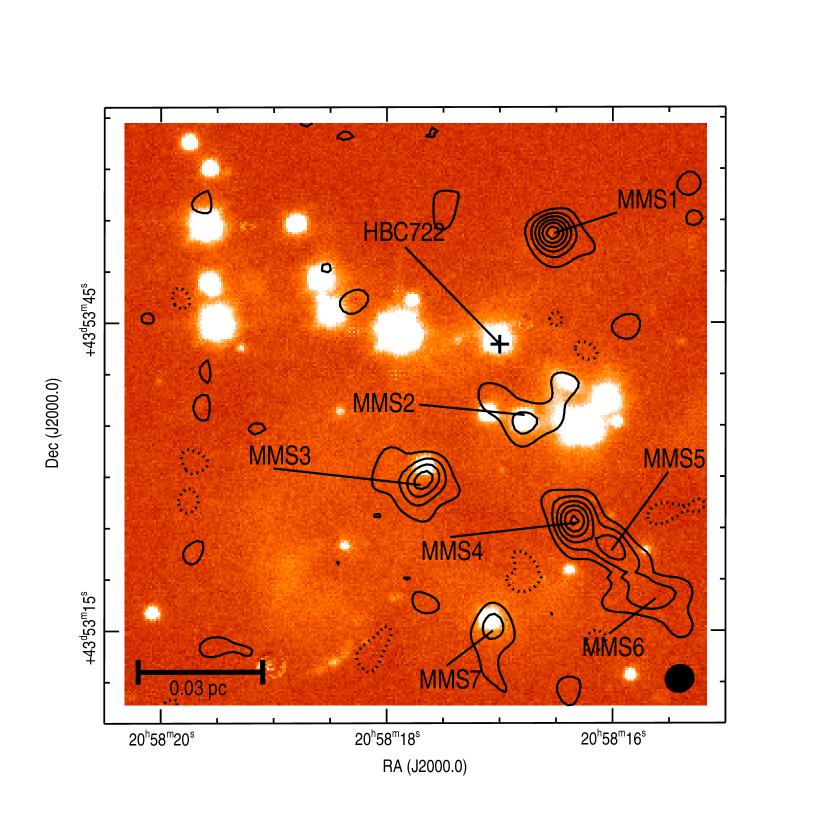
Figure 1.— UKIDSS K_s band image of the vicinity of HBC722, taken from Green et al. (2011). The cross marks the position of HBC722 itself. Overplotted with solid black lines are SMA 1.3 mm emission contours starting at 2$\sigma$ and increasing by 2$\sigma$, where the 1$\sigma$ rms in the continuum image is 1.65 mJy beam^-1. Also plotted with dotted black lines are SMA 1.3 mm emission contours starting at $-$2$\sigma$ and decreasing by 2$\sigma$. The synthesized beam size and shape of the SMA 1.3 mm continuum observations is shown by the black filled oval in the lower right.

The data were inspected, flagged, and calibrated using the MIR software package and imaged, cleaned, and restored using the Multichannel Image Reconstruction, Image Analysis, and Display (MIRIAD) software package configured for the SMA. Since our data are a mosaic of two pointings, we originally tried to use the MIRIAD clean task mossdi appropriate for mosaics. However, mossdi only allows for a single cleaning iteration, and since the region surrounding HBC722 shows complicated morphology, especially in the ¹²CO data (see §4 below), we found the result to be unacceptable since emission from the sidelobes of the dirty beam were very obviously present in our final image independent of the exact cleaning parameters adopted. Thus, we instead cleaned and imaged each of the two pointings separately using the MIRIAD task clean, using an iterative cleaning process where we first cleaned only those regions showing clear emission in the dirty maps and then used those results as input models to further passes of clean applied over the full images. In the first iteration the regions varied from one channel to the next in the molecular line data since the emission morphology is different at different velocities. Finally, we mosaiced together the final images from each of the two pointings. Both pointings were corrected for primary beam attenuation before mosaicing. While all quantitative results in this paper are derived from the mosaics created after such correction, for display purposes the images and figures are created from the mosaics created without such corrections, unless otherwise indicated. Imaging was performed with a robust uv weighting parameter of $+$1. The final maps were re-gridded onto 0.5″ pixels.

Only the continuum and ¹²CO and ¹³CO are detected and discussed in this paper. Table 1 lists, for each of these observations, the frequency of observation, the synthesized beam size and orientation, the total bandwidth, the channel separation (for the lines), and the measured $1\sigma$ rms. For the continuum, the 1$\sigma$ rms is determined by calculating the standard deviation of all off-source pixels. For the spectra, the 1$\sigma$ rms is determined by calculating, for each pixel, the standard deviation of the intensity in each spectral channel outside of the velocity range of $-$20 to 30 km s^-1, and then calculating the mean standard deviation over all pixels.

4. Results

4.1. Continuum

Figure 1 displays the UKIDSS K_s band image of the vicinity of HBC722, taken from Green et al. (2011). Overlaid are contours showing the SMA 1.3 mm continuum intensity. Seven individual millimeter sources are detected and labeled as MMS1 – MMS7 in order of decreasing declination. As evident from this Figure, HBC722 itself is not detected at 1.3 mm. Associations between the seven millimeter sources detected by the SMA and known sources at infrared and submillimeter wavelengths will be discussed in §5.1, and the non-detection of HBC722 itself will be discussed in §5.2.

Table 2Elliptical Gaussian Fits to the 1.3 mm Continuum Detections

	Peak R.A.	Peak Decl.	Peak Flux Density	Total Flux Density	Source Size	Source P.A.	$M$	$n$
Source	(J2000)	(J2000)	(mJy beam-1)	(mJy)	(″)	(degrees)	(M⊙)	(cm-3)
MMS1	20:58:16.52	$+$43:53:53.7	27.4 $\pm$ 6.0	38.3 $\pm$ 7.7	2.0 $\times$ 1.6	$+$26.6	0.15	5.3 $\times$ 107
MMS2	20:58:16.78	$+$43:53:36.0	7.7 $\pm$ 2.1	55.1 $\pm$ 11.0	8.3 $\times$ 6.1	$-$70.4	0.21	1.2 $\times$ 106
MMS3	20:58:17.70	$+$43:53:29.2	18.6 $\pm$ 4.1	66.1 $\pm$ 13.2	4.9 $\times$ 4.3	$+$31.8	0.25	5.3 $\times$ 106
MMS4	20:58:16.32	$+$43:53:25.5	33.2 $\pm$ 7.1	60.5 $\pm$ 12.1	3.3 $\times$ 1.8	$+$30.2	0.23	3.2 $\times$ 107
MMS5	20:58:16.01	$+$43:53:22.8	25.1 $\pm$ 5.5	62.7 $\pm$ 12.5	5.9 $\times$ 1.0	$+$55.6	0.24	3.4 $\times$ 107
MMS6	20:58:15.62	$+$43:53:18.1	15.5 $\pm$ 3.8	44.3 $\pm$ 8.9	6.5 $\times$ 1.6	$+$89.4	0.17	1.0 $\times$ 107
MMS7	20:58:17.06	$+$43:53:15.0	11.0 $\pm$ 2.5	20.3 $\pm$ 4.1	3.1 $\times$ 2.1	$+$1.2	0.08	1.0 $\times$ 107

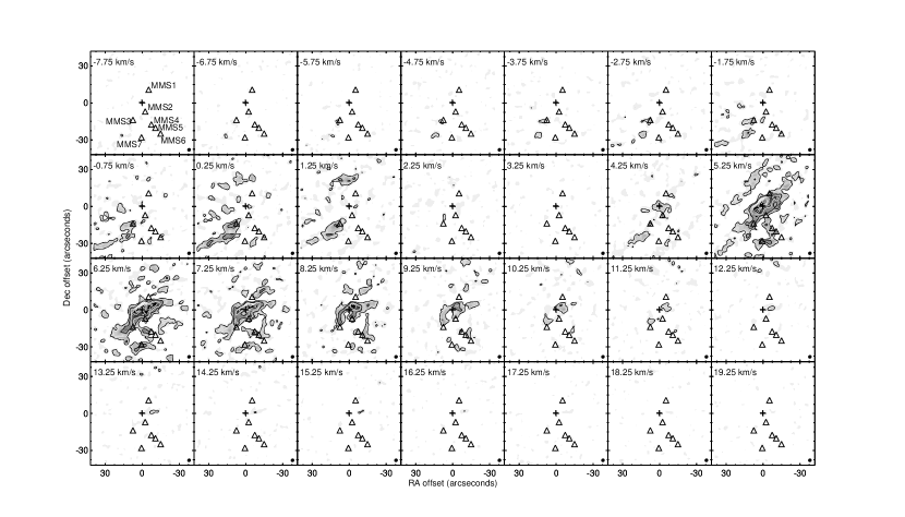
Figure 2.— SMA ¹²CO J $=2-1$ channel maps of the region surrounding HBC722 with a velocity resolution of 1 km s^-1, with the velocities marked in the top left of each panel. The central (0,0) position is that of HBC722 itself and is marked with a cross in each panel. The positions of the 7 sources detected in the SMA 1.3 mm continuum data are plotted as triangles and labeled in the first panel. The gray scale shows intensity in units of Jy beam^-1 with a linear scaling ranging from -0.05 Jy beam^-1 (white) to 4.0 Jy beam^-1 (black). The solid contours start at 5$\sigma$ and increase by 10$\sigma$, where the 1$\sigma$ rms is 0.094 Jy beam^-1 in the 1 km s^-1 channels. The lowest two contours are plotted in black; all others are plotted in white. The dotted contours start at $-$5$\sigma$ and decrease by 10$\sigma$. The synthesized beam size and shape of the ¹²CO J $=2-1$ observations is shown by the black filled oval in the lower right of each panel.

For all seven sources, we used the MIRIAD task imfit to fit an elliptical Guassian to each source. The properties of each source as derived from these fits, including the peak position, peak flux density, total flux density, deconvolved source size, and deconvolved position angle, are reported in Table 2. The last two columns of Table 2 list the mass and density of each source derived from the SMA continuum detections. The mass is calculated as

$$M=100\frac{d^{2}S_{\nu}}{B_{\nu}(T_{D})\kappa_{\nu}}\quad,$$ (1)

where $S_{\nu}$ is the total flux density, $B_{\nu}(T_{D})$ is the Planck function at the isothermal dust temperature $T_{D}$, $\kappa_{\nu}$ is the dust opacity, $d=520$ pc, and the factor of 100 is the assumed gas-to-dust ratio. We adopt the dust opacities of Ossenkopf & Henning (1994) appropriate for thin ice mantles after $10^{5}$ yr of coagulation at a gas density of $10^{6}$ cm^-3 (OH5 dust), giving $\kappa_{\nu}=0.867$ cm² gm^-1 at the frequency of the continuum observations. To calculate the mass we assume $T_{D}=30$ K. No uncertainties are given for the masses because these uncertainties are dominated by uncertain assumptions for the dust temperature and opacity. For example, changing the assumed $T_{D}$ to 10 K would increase the masses by a factor of 4.5. Furthermore, the dust opacity at 1.3 mm can vary by factors of $\sim 2-4$ depending on which dust opacity model is adopted (e.g., Shirley et al. 2005; 2011), directly leading to factors of $\sim 2-4$ variation in the mass.

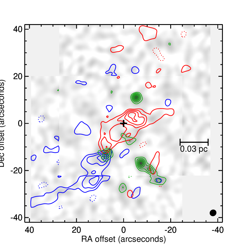
Figure 3.— High-velocity redshifted and blueshifted integrated ¹²CO J $=2-1$ emission overlaid on the SMA 1.3 mm continuum image of the region surrounding HBC722. The central (0,0) position and the black cross mark the position of HBC722 itself. The grayscale is inverted and displayed in a linear stretch ranging from -1.65 mJy beam^-1 ($-1\sigma$, white) to 28.05 mJy beam^-1 ($17\sigma$, black). The solid green contours show the continuum intensity starting at 3$\sigma$ and increasing by 2$\sigma$, where the 1$\sigma$ rms in the continuum image is 1.65 mJy beam^-1. The blue contours show blueshifted ¹²CO J $=2-1$ emission integrated from $-5$ to 1 km s^-1, while the red contours show redshifted emission integrated from 8 to 14 km s^-1. The solid blue and red contours start at 2.0 Jy beam^-1 km s^-1 and increase by 2.0 Jy beam^-1 km s^-1 whereas the dotted blue and red contours start at $-$2.0 Jy beam^-1 km s^-1 and decrease by 2.0 Jy beam^-1 km s^-1. The synthesized beam size and shape of the ¹²CO observations is shown by the black filled oval in the lower right.

The mean number density of each source, $n$, is calculated assuming spherical symmetry as

$$n=\frac{3}{4\pi\mu m_{H}}\frac{M}{r^{3}_{eff}}$$ (2)

where $M$ is the mass, $r_{eff}$ is the effective radius, $m_{H}$ is the hydrogen mass, and $\mu$ is the mean molecular weight per free particle. We adopt $\mu=2.37$ for gas that is 71% by mass hydrogen, 27% helium, and 2% metals (Kauffmann et al. 2008). Again, no uncertainties are listed since they are dominated by the uncertainties in mass.

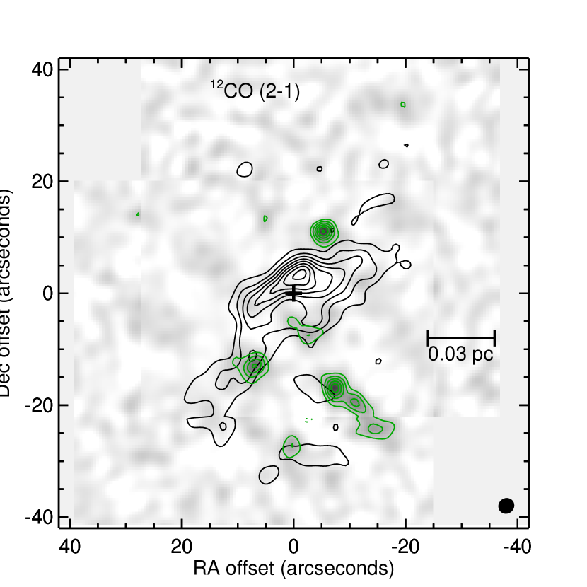
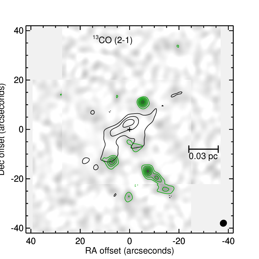
Figure 4.— Low-velocity ¹²CO (left) and ¹³CO (right) integrated emission overlaid on the SMA 1.3 mm continuum image of the region surrounding HBC722. The background images and green contours are the same as described in Figure 3. The black contours show the ¹²CO (left) and ¹³CO (right) emission integrated from 1 to 8 km s^-1. For ¹²CO they start at 3 Jy beam^-1 km s^-1 and increase by 3 Jy beam^-1 km s^-1, while for ¹³CO they start at 1.2 Jy beam^-1 km s^-1 and increase by 1.2 Jy beam^-1 km s^-1. The synthesized beam sizes and shapes of the ¹²CO (left) and ¹³CO (right) observations are shown by the black filled oval in the lower right.

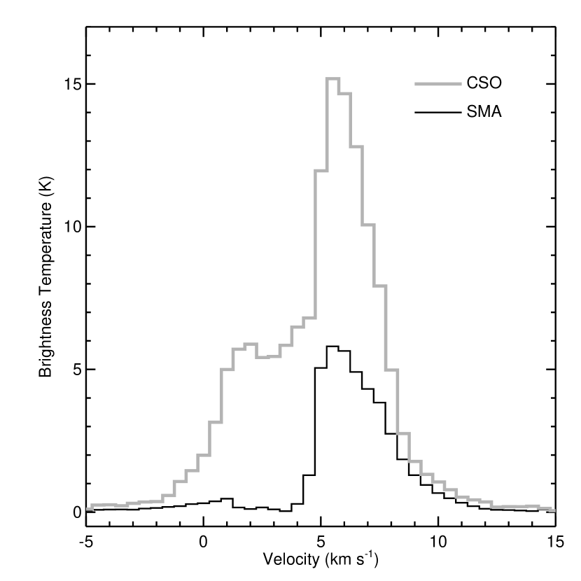
Figure 5.— CSO ¹²CO J $=2-1$ spectrum centered on HBC722 from Green et al. (2011) (gray line) and average SMA ¹²CO J $=2-1$ spectrum centered on HBC722 (black line), with the average weighted by the CSO beam (assumed to be a Guassian with a 32.5″ FWHM).

If we treat sources MMS4, MMS5, and MMS6 as a single group of sources and average their positions to determine the position of the group, the nearest neighbor distance for each of the 5 sources (where MMS4, MMS5, and MMS6 are now a single source) ranges from $0.03-0.045$ pc. This is comparable to the Jeans length of 0.02 – 0.07 pc for 10 K gas at number densities $n=10^{5}-10^{6}$ cm^-3. However, any further interpretation is limited by the fact that we are only able to measure projected separations in the plane of the sky.

4.2. CO

Figure 2 displays channel maps of the SMA ¹²CO J $=2-1$ data at a velocity resolution of 1 km s^-1. Emission is detected between approximately $-5$ to 15 km s^-1. The lack of emission in the channel centered around 3.25 km s^-1 suggests a cloud systemic velocity around this value since the cloud emission is typically fully resolved out in interferometer observations with similar uv coverage to the data presented here. However, with no detections of dense gas tracers, including N₂D⁺ J $=3-2$ in these observations, the true systemic velocity of HBC722 and other, nearby sources in the region is not well characterized. We note that Green et al. (2011) detected ¹²CO J $=14-13$ at a velocity of 6.6 km s^-1 in a Herschel-HIFI (Heterodyne Instrument for the Far-Infrared; de Graauw et al. 2010) observation centered on HBC722, but such a high-J transition may be dominated by warm gas in outflows in the region and not a good tracer of the true cloud systemic velocity.

In single-dish ¹²CO J $=2-1$ data obtained at the CSO, Green et al. (2011) detected a bipolar molecular outflow centered approximately at the position of HBC722, with blueshifted emission extending to the southeast and redshifted emission extending to the northwest. However, with a 32.5″ beam, they lacked the spatial resolution to definitively identify the driving source of this outflow and noted the possibility that none of the detected CO emission was related to HBC722 itself. Figure 3 shows integrated blueshifted and redshifted SMA ¹²CO J $=2-1$ emission contours overlaid on the 1.3 mm continuum image, integrated over the velocity intervals of $-$5 to 1 km s^-1 for the blueshifted emission and 8 to 14 km s^-1 for the redshifted emission. The presence of blueshifted emission extending to the southeast and redshifted emission extending to the northwest is confirmed in the SMA data. The emission is centered on the continuum source MMS3, arguing that it is this source rather than HBC722 that is driving the outflow detected by Green et al. and confirmed by these SMA observations. We also note the presence of weak redshifted emission extending to the northwest of MMS5 in an L-shaped morphology (see, in particular, the 8.25 km s^-1 panel of Figure 2) and weak blueshifted emission extended to the southwest of MMS2 (most noticeable in the 0.25 km s^-1 panel of Figure 2), possibly indicating the presence of an outflow driven by MMS5.

The NW-SE outflow driven by MMS3 shows an S-shaped morphology, similar to that observed in several other sources over a range of masses, including IRAS 20126+4104 (Shepherd et al. 2000), L1157 (Zhang et al. 2000), and RNO43 (Arce & Sargent 2005). This type of morphology is typically explained by an outflow axis that precesses with time. Such precession is generally thought to arise from either tidal interactions between the disk of the source driving the outflow and companion sources or from anisotropic accretion events (e.g., Shepherd et al. 2000). A similar morphology, in particular an apparent change in the axis of the red lobe from one oriented more north-south to one oriented more east-west as distance from the driving source increases, is also hinted at in the single-dish data presented by Green et al. (2011). However, as discussed in more detail below, these SMA observations are only recovering the densest components of a very extended emission morphology, leading to significant uncertainty in the true underlying morphology of this outflow. We conclude that there is tentative but unconfirmed evidence that the axis of the outflow driven by MMS3 is precessing.

High-velocity outflowing gas from MMS3 is not the only source of CO emission in the SMA map. Inspection of Figure 2 clearly shows substantial ¹²CO J $=2-1$ emission between 1 and 8 km s^-1, the lower bounds for the blueshifted and redshifted emission, respectively. Figure 4 plots both ¹²CO J $=2-1$ and ¹³CO J $=2-1$ emission contours integrated between $1-8$ km s^-1. Most of the emission is located along the NW-SE axis of the outflow driven by MMS3 and likely arises from a lower-velocity component of this outflow. However, MMS1, MMS2, and HBC722 are all located near the strongest emission, and neither the spatial resolution nor the emission morphology clearly indicate whether all of this emission is due to the outflow driven by MMS3 or if additional weak, low-velocity outflows are present in this region.

Analysis of the outflow(s) in this region is further complicated by the fact that, with minimum baselines of $\sim 5$ k$\lambda$ (corresponding to spatial scales of 25700 AU at a distance of 520 pc) and less than 2% of the total uv pointings located at projected baselines $<10$ k$\lambda$ (corresponding to spatial scales of 12900 AU at a distance of 520 pc), these observations are not sensitive to extended outflow emission. The ¹²CO J $=2-1$ emission shown in Figures 2 – 4 likely only represents the densest, most compact components of a more extended emission morphology. This statement is confirmed by Figure 2 of Green et al. (2011), which clearly shows large-scale ¹²CO J $=2-1$ emission extending over $>$100″ (52000 AU at the distance of 520 pc). It is further confirmed by Figure 5, which compares the CSO ¹²CO J $=2-1$ spectrum at the position of HBC722 from Green et al. (2011) to the average SMA ¹²CO J $=2-1$ spectrum centered on HBC722, where the average is weighted by the CSO beam (assumed to be a Gaussian with a 32.5″ FWHM) and is calculated in practice in the image plane by adding together all emission within 32.5″ of HBC722 and down-weighting based on the distance from HBC722 with the assumed CSO beam. Comparing the CSO and SMA spectra show that at least 50% of the emission is resolved out over essentially all velocities for which CO emission is detected, and more than 90% is resolved out between $1-4$ km s^-1.

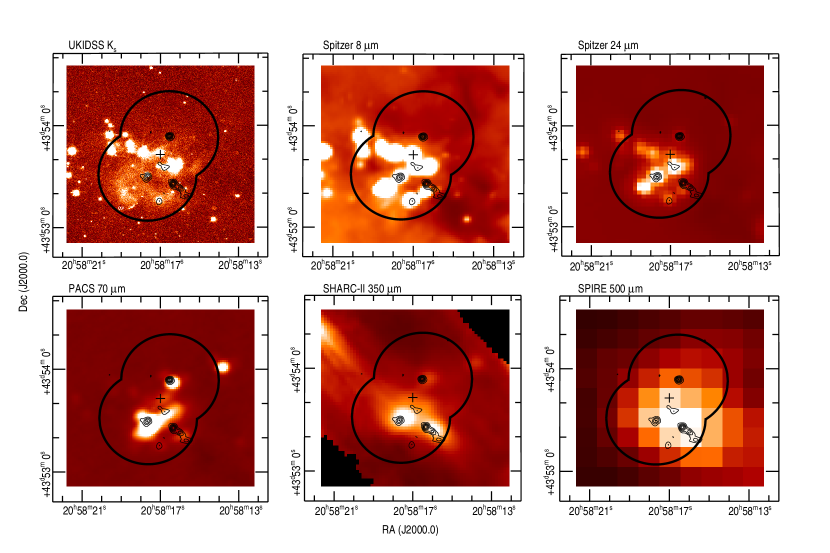
Figure 6.— SMA 1.3mm continuum intensity contours overlaid on infrared and submillimeter images of the region surrounding HBC722. The panels show, from left-to-right and top-to-bottom, UKIDSS K_s band, Spitzer 8 $\mu$m, Spitzer 24 $\mu$m, Herschel 70 $\mu$m, SHARC-II 350 $\mu$m, and Herschel 500 $\mu$m images. The cross in each panel marks the position of HBC722 itself, and the thick black lines show the primary beam of the SMA centered on the two pointings in the mosaic. The thin black lines show the SMA 1.3 mm continuum intensity contours, with the solid lines starting at 3$\sigma$ and increasing by 2$\sigma$ and the dashed lines starting at $-3\sigma$ and decreasing by $2\sigma$, where the 1$\sigma$ rms in the continuum image is 1.65 mJy beam^-1. Pointing offsets on the order of a few arcseconds are visible between the SMA continuum emission and Herschel and SHARC-II continuum emission; these offsets are within the pointing uncertainties of Herschel and SHARC-II and are much smaller than the single-dish beams, thus we consider them to be negligible.

Ultimately, we confirm the presence of at least one NW-SE outflow in the vicinity of HBC722, as suggested by Green et al. (2011). The morphology of this outflow suggests MMS3 rather than HBC722 as the most likely driving source, and suggests that this outflow may be precessing. There is also an extremely tentative detection of a weak outflow driven by MMS5. We do not find any conclusive evidence that HBC722 itself is driving an outflow. Given the uncertainties in the systemic velocity of the region and in the true morphology of the CO emission due to resolving out extended emission, we are unable to completely rule out the possibility of additional outflows in the region, particularly at low velocities relative to the uncertain core systemic velocity. Indeed, we note that there is ¹²CO and ¹³CO emission spatially coincident with HBC722, but lack sufficient information to determine whether its origin lies in one or more outflows or simply in ambient cloud emission. Future observations that provide both higher spatial resolution and better sensitivity to extended emission are required to fully analyze the outflows in the vicinity of HBC722.

5. Discussion

5.1. Continuum Sources

Figure 6 displays infrared and submillimeter images of the HBC722 environment, including an UKIDSS (UKIRT [United Kingdom Infrared Telescope] Infrared Deep Sky Survey) $K_{\rm S}$ image, a Spitzer 8 $\mu$m image from Guieu et al. (2009), a Spitzer 24 $\mu$m image from Rebull et al. (2011), and a Herschel 70 $\mu$m image, SHARC-II 350 $\mu$m image, and Herschel 500 $\mu$m image from Green et al. (2011). Overplotted in black are the SMA 1.3 mm continuum intensity contours and the primary beams of the SMA pointings. A version of this Figure without the SMA 1.3 mm continuum intensity contours was previously presented by Green et al. (2011).

Inspection of Figure 6 shows that most of the seven detected SMA continuum sources are associated with sources at other wavelengths. A detailed discussion of each individual continuum source and its associations with sources at other wavelengths is given below. Table 3 lists, for each source, Spitzer photometry at $3.6-24$ $\mu$m from Guieu et al. (2009) and Rebull et al. (2011), Herschel 70 and 100 $\mu$m photometry from Green et al. (2011), SHARC-II 350 $\mu$m photometry from Green et al. (2011), and SMA 1.3 mm continuum photometry from this work. Figure 7 plots SEDs of all seven continuum sources, including both detections and upper limits (see below for more details).

Table 3Infrared and (Sub)millimeter Photometry of Continuum Sources

Wavelength	MMS1	MMS2	MMS3	MMS4	MMS5	MMS6	MMS7
($\mu$m)	Sν (mJy)	Sν (mJy)	Sν (mJy)	Sν (mJy)	Sν (mJy)	Sν (mJy)	Sν (mJy)
3.6	$<$0.6	17.4 $\pm$ 0.9	5.61 $\pm$ 0.28	$<$0.6	$<$0.6	$<$0.6	13.6 $\pm$ 0.68
4.5	$<$0.6	25.5 $\pm$ 1.3	10.9 $\pm$ 0.55	$<$0.6	$<$0.6	$<$0.6	25.7 $\pm$ 1.3
5.8	$<$0.6	35.4 $\pm$ 1.8	14.5 $\pm$ 0.72	$<$0.6	$<$0.6	$<$0.6	30.2 $\pm$ 1.5
8.0	$<$0.6	58.0 $\pm$ 2.9	20.1 $\pm$ 1.0	$<$0.6	$<$0.6	$<$0.6	38.6 $\pm$ 1.9
24	41.1 $\pm$ 4.1	303 $\pm$ 30	219 $\pm$ 22	$<$2.8	$<$2.8	$<$2.8	76.2 $\pm$ 3.8
70	1250 $\pm$ 130	1260 $\pm$ 130	6730 $\pm$ 680	$<$90	369 $\pm$ 42	$<$151	179 $\pm$ 22
100	2230 $\pm$ 230	2250 $\pm$ 230	9530 $\pm$ 960	$<$712	1290 $\pm$ 130	$<$1020	$<$458
350	2700 $\pm$ 500	$<$2800	12000 $\pm$ 2400	$<$4000	10000 $\pm$ 2000	$<$3000	$<$720
1300	38.3 $\pm$ 7.7	55.1 $\pm$ 11	66.1 $\pm$ 13	60.5 $\pm$ 12	62.7 $\pm$ 13	44.3 $\pm$ 8.9	20.3 $\pm$ 4.1

Figure 7.— Spectral Energy Distributions (SEDs) for each of the seven detected continuum sources, consisting of Spitzer $3.6-24$ $\mu$m data, Herschel 70 and 100 $\mu$m data, SHARC-II 350 $\mu$m data, and the SMA 1.3 mm continuum data (see text for details). Detections are plotted as filled circles with error bars and upper limits are plotted as open triangles. Each panel is labeled with the corresponding source.

Table 4Evolutionary Indicators

		$T_{bol}$	$L_{bol}$
Source	$\alpha$	(K)	(L⊙)
MMS1	$\cdots$	39	1.1
MMS2	0.49	147	1.5
MMS3	0.76	52	5.9
MMS4	$\cdots$	$\cdots$	$\cdots$
MMS5	$\cdots$	15	1.4
MMS6	$\cdots$	$\cdots$	$\cdots$
MMS7	$-$0.20	328	0.3

Table 4 presents three evolutionary indicators for each source calculated from the SEDs tabulated in Table 3 and plotted in Figure 7: the infrared spectral index ($\alpha$), the bolometric temperature ($T_{bol}$), and the bolometric luminosity ($L_{bol}$). As first defined by Lada & Wilking (1984) and Lada (1987), $\alpha$ is the infrared slope in log space of $\nu S_{\nu}$ vs. $\nu$ and is used to classify sources into different evolutionary stages (see Evans et al. [2009] for a recent review of classification via $\alpha$). In this study we calculate $\alpha$ with a linear least-squares fit to all available Spitzer photometry between $3.6-24$ $\mu$m. $T_{bol}$ is defined as the temperature of a blackbody with the same flux-weighted mean frequency as the source SED (Myers & Ladd 1993) and provides an alternative classification method to $\alpha$ (Chen et al. 1995; Evans et al. 2009). We calculate both $T_{bol}$ and $L_{bol}$ by using the trapezoid rule to integrate over the finely sampled SEDs; a detailed description of the implementation of this method and resulting errors due to the finite sampling of the observed SEDs is given in Appendix B of Dunham et al. (2008). An additional error is introduced by the fact that the SMA 1.3 mm continuum data resolve out some of the emission from the extended core and are thus lower limits to the true flux densities at this wavelength, artifically steepening the far-infrared and submillimeter slope of the SEDs. The magnitude of the error introduced depends on both the amount of emission recovered by the SMA and the spectral shape of each source; a very conservative estimate that only 1% of the emission is recovered leads to underestimates in $L_{bol}$ by less than a factor of 2 for all sources, and less than 50% for all but MMS7. Thus, while we caution that the calculated $L_{bol}$ may underestimate the true values, the magnitude of these underestimates are likely comparable to or less than the other errors discussed by Dunham et al. (2008).

Finally, we note that there are three other infrared sources identified as Spitzer-detected Young Stellar Objects by Guieu et al. (2009) and Rebull et al. (2011) covered by our SMA observations, and several other infrared sources covered that are not identified as Young Stellar Objects and are thus likely background or foreground stars. As our focus is on providing a high spatial resolution view of the millimeter emission in the vicinity of HBC722 we do not discuss these sources further except to note that their non-detections in our SMA 1.3 mm continuum observations suggest similar upper limits to the masses of any circumstellar disks surrounding these objects as for HBC722 itself, which we discuss below in §5.2.

5.1.1 MMS1

MMS1 is associated with the Spitzer infrared source SST J205816.56$+$435352.9 from Guieu et al. (2009) and Rebull et al. (2011). It is detected by Spitzer only at 24 $\mu$m with the flux density listed in Table 3. The Spitzer $3.6-8$ $\mu$m upper limits listed are taken from Guieu et al. (2009); they note that their 90% completeness limits increase from about 0.3 mJy at 3.6 $\mu$m to 0.6 mJy at 8 $\mu$m but do not specifically list these limits for 4.5 and 5.8 $\mu$m, thus we conservatively take the upper limits to be 0.6 mJy in all four bands. MMS1 is also associated with a Herschel source detected at 70 and 100 $\mu$m from Green et al. (2009); all other Herschel wavelengths are of too low spatial resolution ($18-35$″ at $160-500$ $\mu$m) to accurately separate the 7 continuum sources and are not considered in this study. The 70 and 100 $\mu$m photometry presented in Table 3 is calculated with 10″ diameter apertures chosen as the best compromise between including as much source flux as possible and excluding flux from other, nearby sources. No aperture or color corrections are applied since neither the true spatial profile of the emission nor the underlying spectral shape of any source is known. Finally, MMS1 is also associated with a SHARC-II 350 $\mu$m source. The photometry presented in Table 3 is calculated in a 20″ diameter aperture following the method described by Wu et al. (2007).

The SED of MMS1 resembles that of a deeply embedded protostar. We are unable to calculate $\alpha$ with only one Spitzer detection, but the upper limits are consistent with a positive $\alpha$ indicative of a Class 0/I object. We calculate $T_{bol}$ $=39$ K, placing MMS1 in Class 0, consistent with the above statements. We thus conclude that MMS1 is a deeply embedded Class 0 protostar. As described in §4.2 above, we do not detect clear signatures of an outflow driven by MMS1 but do note that there may be additional outflows in this region that are not fully separated spatially and kinematically by these data.

5.1.2 MMS2

MMS2 is associated with the Spitzer infrared source SST J205816.8$+$435335.6 from Guieu et al. (2009) and Rebull et al. (2011) and is detected at all five Spitzer wavelengths from $3.6-24$ $\mu$m. It is also detected at 70 and 100 $\mu$m with Herschel. The photometry is again calculated in 10″ diameter apertures and is uncertain since the apertures do not fully capture the emission that extends to the northwest but also partially overlap with the emission from the brighter MMS3. More accurate photometry at these wavelengths will require higher-resolution observations. There is no clear SHARC-II 350 $\mu$m source, but the position of MMS2 overlaps with bright emission from MMS3 and MMS5. We calculate the upper limit as the flux in one beam at the position of MMS2 from the other, nearby sources.

The SED of MMS2 resembles that of a Class I protostar more evolved and less deeply embedded than MMS1. The calculated values of $\alpha$ and $T_{bol}$ (0.49 and 147 K, respectively) both classify MMS2 as Class I, confirming this statement.

5.1.3 MMS3

MMS3 is associated with the Spitzer infrared source SST J205817.7$+$435331.1 from Guieu et al. (2009) and Rebull et al. (2011) and is detected at $3.6-24$ $\mu$m with Spitzer. It is also detected at 70 and 100 $\mu$m with Herschel and 350 $\mu$m with SHARC-II and is the brightest source in the region at these wavelengths. The photometry at 70, 100, and 350 $\mu$m is calculated with apertures and methods identical to MMS1 above. The true flux densities at these wavelengths are likely higher than the values listed in Table 3 since the apertures do not include all of the extended emission, but larger apertures are not feasible since they would overlap with other, nearby sources.

As with MMS1, the SED of MMS3 resembles that of a deeply embedded protostar. The calculated values of both $\alpha$ (0.76; in the Class 0/I category) and $T_{bol}$ (52 K; in the Class 0 category) are consistent with this observation. As discussed in §4.2 above, MMS3 is driving a NW-SE outflow detected both by the SMA ¹²CO J $=2-1$ observations presented here and single-dish ¹²CO J $=2-1$ observations presented by Green et al. (2011). The axis of this outflow may be precessing over time.

5.1.4 MMS4

MMS4 is not associated with a Spitzer infrared source at $3.6-24$ $\mu$m, it is not associated with a Herschel infrared source at 70 and 100 $\mu$m, and it is not associated with a SHARC-II 350 $\mu$m submillimeter source. The upper limits for $3.6-8$ $\mu$m are again taken from Guieu et al. (2009) as described above for MMS1. For 24 $\mu$m, we take the upper limit to be the point at which the source count histogram presented in Figure 9 of Rebull et al. (2011) turns over, which we estimate to be at a magnitude of 8.5 (corresponding to a flux density of 2.8 mJy). While there is no Herschel 70 or 100 $\mu$m source or SHARC-II 350 $\mu$m source, there is emission at the position of MMS4 from the brighter nearby sources (MMS3 and MMS5). Thus, similar to MMS2 above, we calculate the upper limits as the flux in one beam at the position of MMS4 from other, nearby sources.

With no detections of a compact, infrared source in any of the Spitzer bands, and also no detections at $70-350$ $\mu$m, MMS4 is possibly a starless core heated only externally and thus too faint to detect at 350 $\mu$m above the emission from nearby, brighter sources. The 350 $\mu$m upper limit of 4 Jy is consistent with this statement since starless cores and cores containing very low luminosity protostars are typically less than 1 – 2 Jy at this wavelength (Wu et al. 2007). However, recent work suggests that detections of starless cores with current interferometers are extremely rare since starless cores are not yet very centrally condensed and are thus fully resolved out (Schnee et al. 2010; Offner et al. 2012). If MMS4 is indeed a starless core, the SMA detection indicates it may be very evolved and close to the onset of star formation. Alternatively, star formation may have already begun, with the core harboring a very young, very low luminosity protostar or first hydrostatic core. Confirmation would require either the detection of a very faint infrared source below the detection limits of the data considered here, such as the 70 $\mu$m detection of the source Per-Bolo 58 presented by Enoch et al. (2010), or the detection of a molecular outflow driven by this core, such as the detections of outflows from cores previously believed to be starless presented by Chen et al. (2010), Dunham et al. (2011), Pineda et al. (2011), and Schnee et al. (2012). No such outflow is detected in our ¹²CO J $=2-1$ observations, but this topic should be revisited with future observations providing higher sensitivity and higher spatial resolution.

5.1.5 MMS5

MMS5 is not associated with a Spitzer infrared source at $3.6-24$ $\mu$m, and the upper limits listed in Table 3 are determined as described above. MMS5 is associated with a source detected at 70 and 100 $\mu$m with Herschel and 350 $\mu$m with SHARC-II, and the photometry at these wavelengths is calculated with apertures and methods identical to MMS1 above. The SED of MMS5 resembles that of a Class 0 protostar too deeply embedded to be detected in the mid-infrared with Spitzer. With no such detections we are unable to calculate $\alpha$, but calculate a value for $T_{bol}$ (15 K) consistent with that of a Class 0 source. As noted in §4.2, there is weak redshifted emission extending to the northwest of MMS5 and weak blueshifted emission to the southeast. These weak features may be due to an outflow driven by MMS5, but higher sensitivity ¹²CO observations are required to confirm this tentative outflow.

5.1.6 MMS6

Similar to MMS4, MMS6 is not associated with a Spitzer infrared source at $3.6-24$ $\mu$m, it is not associated with a Herschel infrared source at 70 and 100 $\mu$m, and it is not associated with a SHARC-II 350 $\mu$m submillimeter source. The $3.6-24$ $\mu$m upper limits listed in Table 3 are determined as described above. The 70, 100, and 350 $\mu$m upper limits are calculated as the flux in one beam at the position of MMS6 from other, nearby sources. The same discussion presented above for the evolutionary status of MMS4 also applies for MMS6; it is likely either an evolved starless core close to the onset of star formation or a very young, very low luminosity protostar or first hydrostatic core. As with MMS4, we do not detect any evidence for an outflow driven by MMS6.

5.1.7 MMS7

MMS7 is associated with the Spitzer infrared source SST J205817.06$+$435316.1 from Guieu et al. (2009) and Rebull et al. (2011) and is detected at all five Spitzer wavelengths. It is also detected at 70 $\mu$m with Herschel, and the photometry presented in Table 3 is calculated with an aperture and methods identical to MMS1 above. It is not detected at either 100 $\mu$m with Herschel or 350 $\mu$m with SHARC-II; upper limits are again calculated as the flux in one beam at the position of MMS7 from other, nearby sources. The SED of MMS7 resembles that of a young stellar object (YSO) surrounded by a circumstellar disk but no longer embedded within a dense core; the calculated values of $\alpha$ ($-$0.20; in the Flat Spectrum category) and $T_{bol}$ (328 K; near the Class I/II boundary) confirm this assessment.

5.2. Evolutionary Status of HBC722

Prior to outburst HBC722 was regarded as a Class II T Tauri star with a spectral type of K7$-$M0, a mass of $\sim 0.5-0.6$ M_⊙, a visual extinction of 3.4 magnitudes, an infrared spectral index of $-0.77$, and a bolometric luminosity of 0.85 L_⊙ (Cohen & Kuhi 1979; Kóspál et al. 2011; Miller et al. 2011). As noted in §4.1, HBC722 itself is not detected in our SMA 1.3 mm continuum observations down to a $3\sigma$ upper limit of 5 mJy beam^-1. Under the same assumptions as discussed above in §4.1, this corresponds to an upper limit of 0.02 M_⊙ for the disk mass (lower if the disk is warmer than 30 K) and an upper limit of 3% – 4% for the ratio of disk to stellar mass (again, lower if the disk is actually warmer than 30 K). In a large submillimeter survey of circumstellar disks around young stars, Andrews & Williams (2005) report a mean disk mass of 0.005 M_⊙ with a large dispersion of $\sim$0.5 dex, and a median ratio of disk to stellar mass of 0.5%. Thus, our observations do not rule out the presence of a typical mass disk.

In a typical FUor flare with an accretion rate of 10^-4 M_⊙ yr^-1 and a duration of 100 yr, up to 0.01 M_⊙ of mass can accrete from the disk onto the protostar. For HBC722, however, Kóspál et al. (2011) calculated a burst accretion rate of only 10^-6 based on their measured $L_{bol}$ during the burst. Our derived upper limit for the disk mass of 0.02 M_⊙ is thus consistent with providing a sufficient mass reservoir to support the observed outburst in HBC722 unless the accretion rate is several orders of magnitude higher than estimated by Kóspál et al. and/or the burst duration is much longer than the typical 100 yr. Even if one of these cases were true, there is possibly gas remaining in the vicinity of HBC722 that could still accrete onto the star+disk system and power the burst, as suggested by ¹³CO J $=2-1$ and Herschel far-infrared continuum emission spatially coincident with HBC722. Further constraints on the amount of circumstellar mass available to accrete onto HBC722 and the likelihood of sufficient mass remaining to power further bursts beyond the current one require deeper millimeter continuum data probing to lower disk masses and higher-resolution far-infrared and submillimeter continuum data observed during the burst to better determine the burst luminosity and implied accretion rate. For the former, the high sensitivity of full-science ALMA operations will be the ideal facility despite the high declination of HBC722 ($+$44^∘) since, according to the ALMA sensitivity calculator, even a short, 30 minute track with 50 antennas will improve the mass sensitivity by a factor of 100. For the latter, the upcoming 25-m submillimeter telescope CCAT will be of particular value assuming the burst is still in progress when CCAT begins science operations (currently expected in 2015 – 2017; Radford et al. 2009; Sebring 2010).

6. Summary

In this paper we have presented 230 GHz Submillimeter Array continuum and molecular line observations of the newly discovered FUor candidate HBC722. We summarize our main results as follows.

1. Seven 1.3 mm continuum sources are detected in the vicinity of HBC722; none are HBC722 itself. We compile infrared and submillimeter continuum photometry of each source from previous studies and conclude that three are Class 0 embedded protostars, one is a Class I embedded protostar, one is a Class I/II transition object, and two are either starless cores or very young, very low luminosity protostars or first hydrostatic cores.

2. A northwest-southeast outflow is detected in the ¹²CO J $=2-1$ observations. This outflow is centered on and thus likely driven by MMS3, one of the Class 0 sources detected in the 1.3 mm continuum data, and its axis may be precessing. This outflow detection is consistent with a similar outflow detected in low-resolution, single-dish ¹²CO J $=2-1$ observations presented by Green et al. (2011). Our higher spatial resolution confirms that HBC722 is not the driving source.

3. There is no conclusive evidence that HBC722 itself is driving an outflow, although we caution that higher spatial resolution, better sensitivity to extended emission, and better determinations of the systemic velocities of the sources in the vicinity of HBC722 are needed to fully evaluate the kinematics of the ¹²CO J $=2-1$ gas in this region.

4. The non-detection of HBC722 in the 1.3 mm continuum observations suggests an upper limit of 0.02 M_⊙ for the mass of the circumstellar disk, consistent with typical T Tauri disks. This upper limit is consistent with a disk that provides sufficient mass to power the burst. Future observations are needed to further study the actual amount of circumstellar mass available to accrete onto HBC722 and the likelihood of sufficient mass remaining to power additional bursts beyond the current one.

We have noted in the text several future observations that are needed in order to better disentangle the millimeter emission in this complicated environment and better determine the properties and evolutionary status of HBC722.

References

- (1)
- (2) Andrews, S. M., & Williams, J. P. 2005, ApJ, 631, 1134
- (3)
- (4) Arce, H. G., & Sargent, A. I. 2005, ApJ, 624, 232
- (5)
- (6) Bonnell, I., & Bastien, P. 1992, ApJ, 401, L31
- (7)
- (8) Chen, H., Myers, P. C., Ladd, E. F., & Wood, D. O. S. 1995, ApJ, 445, 377
- (9)
- (10) Chen, X., Arce, H. G., Zhang, Q., et al. 2010, ApJ, 715, 1344
- (11)
- (12) Cohen, M., & Kuhi, L. V. 1979, ApJS, 41, 743
- (13)
- (14) de Graauw, T., Helmich, F. P., Phillips, T. G., et al. 2010, A&A, 518, L6
- (15)
- (16) Dunham, M. M., Crapsi, A., Evans, N. J., II, et al. 2008, ApJS, 179, 249
- (17)
- (18) Dunham, M. M., Evans, N. J., II, Terebey, S., Dullemond, C. P., & Young, C. H. 2010, ApJ, 710, 470
- (19)
- (20) Dunham, M. M., Chen, X., Arce, H. G., et al. 2011, ApJ, 742, 1
- (21)
- (22) Dunham, M. M., & Vorobyov, E. I. 2012, ApJ, 747, 52
- (23)
- (24) Enoch, M. L., Evans, N. J., II, Sargent, A. I., & Glenn, J. 2009, ApJ, 692, 973
- (25)
- (26) Enoch, M. L., Lee, J.-E., Harvey, P., Dunham, M. M., & Schnee, S. 2010, ApJ, 722, L33
- (27)
- (28) Evans, N. J., II, Dunham, M. M., Jørgensen, J. K., et al. 2009, ApJS, 181, 321
- (29)
- (30) Fazio, G. G., Hora, J. L., Allen, L. E., et al. 2004, ApJS, 154, 10
- (31)
- (32) Green, J. D., Evans, N. J., II, Kóspál, Á., et al. 2011, ApJ, 731, L25
- (33)
- (34) Guieu, S., Rebull, L. M., Stauffer, J. R., et al. 2009, ApJ, 697, 787
- (35)
- (36) Hartmann, L., & Kenyon, S. J. 1985, ApJ, 299, 462
- (37)
- (38) Hartmann, L., & Kenyon, S. J. 1996, ARA&A, 34, 207
- (39)
- (40) Herbig, G. H. 1966, Vistas in Astronomy, 8, 109
- (41)
- (42) Herbig, G. H. 1977, ApJ, 217, 693
- (43)
- (44) Ho, P. T. P., Moran, J. M., & Lo, K. Y. 2004, ApJ, 616, L1
- (45)
- (46) Kauffmann, J., Bertoldi, F., Bourke, T. L., Evans, N. J., II, & Lee, C. W. 2008, A&A, 487, 993
- (47)
- (48) Kenyon, S. J., Hartmann, L. W., Strom, K. M., & Strom, S. E. 1990, AJ, 99, 869
- (49)
- (50) Kóspál, Á., Ábrahám, P., Acosta-Pulido, J. A., et al. 2011, A&A, 527, A133
- (51)
- (52) Lada, C. J., & Wilking, B. A. 1984, ApJ, 287, 610
- (53)
- (54) Lada, C. J. 1987, IAU Symp. 115: Star Forming Regions (Dordrecht: Kluwer), a
- (55)
- (56) Laugalys, V., Straižys, V., Vrba, F. J., et al. 2006, Baltic Astronomy, 15, 483
- (57)
- (58) Leoni, R., Larionov, V. M., Centrone, M., Giannini, T., & Lorenzetti, D. 2010, The Astronomer’s Telegram, 2854, 1
- (59)
- (60) Lorenzetti, D., Antoniucci, S., Giannini, T., et al. 2012, ApJ, in press, arXiv:1202.4136
- (61)
- (62) Miller, A. A., Hillenbrand, L. A., Covey, K. R., et al. 2011, ApJ, 730, 80
- (63)
- (64) Munari, U., Milani, A., Valisa, P., & Semkov, E. 2010, The Astronomer’s Telegram, 2808, 1
- (65)
- (66) Myers, P. C., & Ladd, E. F. 1993, ApJ, 413, L47
- (67)
- (68) Offner, S. S. R., Capodilupo, J., Schnee, S., & Goodman, A. A. 2012, MNRAS, 420, L53
- (69)
- (70) Pilbratt, G. L., Riedinger, J. R., Passvogel, T., et al. 2010, A&A, 518, L1
- (71)
- (72) Pineda, J. E., Arce, H. G., Schnee, S., et al. 2011, ApJ, 743, 201
- (73)
- (74) Radford, S. J. E., Giovanelli, R., Sebring, T. A., & Zmuidzinas, J. 2009, Submillimeter Astrophysics and Technology: a Symposium Honoring Thomas G. Phillips, 417, 113
- (75)
- (76) Rebull, L. M., Guieu, S., Stauffer, J. R., et al. 2011, ApJS, 193, 25
- (77)
- (78) Reipurth, B. & Aspin, C. 2010, in Evolution of Cosmic Objects through their Physical Activity, ed. H. A. Harutyunian, A. M. Mickaelian, & Y. Terzian, 19–38
- (79)
- (80) Rieke, G. H., Young, E. T., Engelbracht, C. W., et al. 2004, ApJS, 154, 25
- (81)
- (82) Schnee, S., Enoch, M., Johnstone, D., et al. 2010, ApJ, 718, 306
- (83)
- (84) Schnee, S., Di Francesco, J., Enoch, M., et al. 2012, ApJ, 745, 18
- (85)
- (86) Sebring, T. 2010, Proc. SPIE, 7733,
- (87)
- (88) Semkov, E. H., Peneva, S. P., Munari, U., Milani, A., & Valisa, P. 2010, A&A, 523, L3
- (89)
- (90) Semkov, E., & Peneva, S. 2010a, The Astronomer’s Telegram, 2801, 1
- (91)
- (92) Semkov, E., & Peneva, S. 2010b, The Astronomer’s Telegram, 2819, 1
- (93)
- (94) Semkov, E. H., Peneva, S. P., Munari, U., et al. 2012, A&A, 542, A43
- (95)
- (96) Shepherd, D. S., Yu, K. C., Bally, J., & Testi, L. 2000, ApJ, 535, 833
- (97)
- (98) Shirley, Y. L., Nordhaus, M. K., Grcevich, J. M., et al. 2005, ApJ, 632, 982
- (99)
- (100) Shirley, Y. L., Huard, T. L., Pontoppidan, K. M., et al. 2011, ApJ, 728, 143
- (101)
- (102) Straizys, V., Meistas, E., Vansevicius, V., & Goldberg, E. P. 1989, A&A, 222, 82
- (103)
- (104) Vorobyov, E. I. 2009, ApJ, 704, 715
- (105)
- (106) Vorobyov, E. I., & Basu, S. 2010, ApJ, 719, 1896
- (107)
- (108) Wachmann, A. 1954, ZAp, 35, 74
- (109)
- (110) Werner, M. W., Roellig, T. L., Low, F. J., et al. 2004, ApJS, 154, 1
- (111)
- (112) Wu, J., Dunham, M. M., Evans, N. J., II, Bourke, T. L., & Young, C. H. 2007, AJ, 133, 1560
- (113)
- (114) Zhang, Q., Ho, P. T. P., & Wright, M. C. H. 2000, AJ, 119, 1345
- (115)
- (116) Zhu, Z., Hartmann, L., Calvet, N., et al. 2007, ApJ, 669, 483
- (117)
- (118) Zhu, Z., Espaillat, C., Hinkle, K., et al. 2009, ApJ, 694, L64
- (119)
- (120) Zhu, Z., Hartmann, L., & Gammie, C. 2009, ApJ, 694, 1045
- (121)