Molecular and atomic line surveys of galaxies I:
The dense, star-forming phase as a beacon

Abstract

We predict the space density of molecular gas reservoirs in the Universe, and place a lower limit on the number counts of carbon monoxide (CO), hydrogen cyanide (HCN) molecular and [C ii] atomic emission lines in blind redshift surveys in the submillimeter–centimeter spectral regime. Our model uses: (a) recently available HCN Spectral Line Energy Distributions (SLEDs) of local Luminous Infrared Galaxies (LIRGs, $L_{\rm IR}>10^{11}L_{\odot}$), (b) a value for $\epsilon_{\star}$=$\rm SFR$/$M_{\rm dense}(\rm H_{2})$ provided by new developments in the study of star formation feedback on the interstellar medium and (c) a model for the evolution of the infrared luminosity density. Minimal ‘emergent’ CO SLEDs from the dense gas reservoirs expected in all star-forming systems in the Universe are then computed from the HCN SLEDs since warm, HCN-bright gas will necessarily be CO-bright, with the dense star-forming gas phase setting an obvious minimum to the total molecular gas mass of any star-forming galaxy. We include [C ii] as the most important of the far-infrared cooling lines. Optimal blind surveys with the Atacama Large Millimeter Array (ALMA) could potentially detect very distant ($z\sim 10$–$12$) [C ii] emitters in the $\geq$ULIRG galaxy class at a rate of $\sim$0.1–1 per hour (although this prediction is strongly dependent on the star formation and enrichment history at this early epoch), whereas the (high-frequency) Square Kilometer Array (SKA) will be capable of blindly detecting $z>3$ low-J CO emitters at a rate of $\sim$40–70 per hour. The [C ii] line holds special promise for the detection of metal-poor systems with extensive reservoirs of CO-dark molecular gas where detection rates with ALMA can reach up to 2–7 per hour in Bands 4–6.

1. Introduction

Since the first detections of the $J$$=$$1$$\rightarrow$$0$ rotational transition of ¹²CO and some of its isotopologues in Galactic molecular clouds (¹³CO, C¹⁸O) (Wilson et al. 1970; Penzias et al. 1971, 1972), and in galactic nuclei (Rickard et al. 1975) there have been many studies of CO line emission in galaxies using single dish radio telescopes and interferometer arrays (for reviews see Young & Scoville 1991 and Solomon & Vanden Bout 2005). Multi-J CO line ratio surveys are now routinely used to assess the state of the molecular gas in galaxies (e.g. Braine & Combes 1992; Aalto et al. 1995; Papadopoulos & Seaquist 1998; Mauersberger et al. 1999; Nieten et al. 1999; Yao et al. 2003; Mao et al. 2011) over the density regime where most of its mass resides ($n\sim 10^{2-3}\,{\rm cm}^{-3}$). The fainter molecular line emission from heavy-rotor molecules such as HCN have also become a standard tool for assesing the state and the mass of the denser ($>$$10^{4}\,{\rm cm}^{-3}$) gas phase where stars actually form in Giant Molecular Clouds (GMCs, e.g. Nguyen-Q-Rieu et al. 1989; Solomon et al. 1992a; Paglione et al. 1995, 1997; Jackson et al. 1995). The role of the latter phase as the direct fuel of star formation in individual GMCs, quiescent disks and merger-driven spectacular starbursts in the local and distant Universe is now well established over an astounding 7–8 orders of magnitude (Gao & Solomon 2004; Wu et al. 2005; Juneau et al. 2009; Wang et al. 2011).

In the past decade, numerous high-z detections have revealed the fundamental role of molecular lines in assessing the state and mass of the molecular gas, and the dynamical mass of heavily dust-enshrouded galaxies in the early Universe (Solomon & Vanden Bout 2005 and references therein), and in some cases have provided remarkable insights into the properties of the molecular interstellar medium (ISM) in early galaxies (see Danielson et al. 2010 for a recent example of a well sampled CO spectral line energy distribution (SLED) in a $z=2.3$ gravitationally lensed galaxy). This exploration began with the first detection of  CO J($3$$\rightarrow$$2$)  line emission in the strongly-lensed distant dust-enshrouded galaxy IRAS 10214+4724 at $z\sim 2.3$ (Brown & Vanden Bout 1991; Solomon et al. 1992b). It continued with the detection of CO transitions in distant submm-bright galaxies (SMGs, $L_{\rm IR}>10^{12}L_{\odot}$) (Frayer et al. 1998, 1999; Greve et al. 2005) and is increasingly encompassing less extreme, but still massive systems such as Lyman Break galaxies (Baker et al. 2004), optical/near-infrared selected galaxies at $z\sim 1.5$ (Dannerbauer et al. 2009; Daddi et al. 2010) and fortuitously lensed systems (Danielson et al. 2011; Lupu et al. 2011). Several spectacular CO line detections have also been obtained also for other high-redshift systems such as radio galaxies (e.g. De Breuck et al. 2005) and QSOs out to $z\sim 6.4$. This epoch is close to the era of reionization – the final frontier of galaxy evolution studies – revealing the gas-rich hosts to rapid galaxy growth at these early times (Walter et al. 2003, 2004; Weiss et al. 2007).

These discoveries and advancements, made possible as sensitivities of millimeter/submillimeter interferometer arrays improved in the last decade, still yield only a glimpse of what will be a new era where molecular and atomic (e.g. [C ii]  $\lambda 158$,  [C i](${}^{3}P_{1}$$\rightarrow^{3}$$P_{0}$) ) ISM lines will replace nebular optical/near-infrared (OIR) lines as the main tool of choice for discerning galaxy formation and evolution across the full span of cosmic time pertinent to galaxy growth, from the end of the reionisation epoch ($z>7$) to the present (Walter & Carilli 2008).

Direct ‘blind’ searches of gas-rich galaxies using submm–cm wave molecular and atomic lines are the only tool that can: (i) uniformly select galaxies according to their molecular gas content rather than their SFR and the star formation efficiency (a bias that has so far – necessarily – affected all high-$z$ gas studies), (ii) immediately provides redshifts and eventually dynamical mass information, (iii) holds the promise of discovering large outliers of the local $\Sigma_{\rm SFR}$-$\Sigma_{{\rm H}_{2}}$ (Schmidt–Kennicutt) relations (Kennicutt 1998), with large reservoirs of molecular gas but low levels of SFR (Papadopoulos & Pelupessy 2010), and (iv) can possibly determine the star formation ‘mode’ (starburst/merger-driven versus quiescent/disk-like), in a uniform and extinction-free manner (Paper II, Papadopoulos & Geach 2012).

Well-sampled CO spectral line energy distributions, and their robust normalization by some observable galaxy property are necessary for predicting the emergent CO line luminosities in star-forming systems. The lack of these two key ingredients translates to major uncertainties for the source counts predicted for blank-field cm/mm/submm molecular line surveys (Combes et al. 1999; Blain et al. 2000; Carilli & Blain 2002), as well as the frequency and flux range where such surveys become optimal (Blain et al. 2000). The dense gas phase ($n({\rm H}_{2})$$>$10⁴ cm^-3) and the linear relation of its mass to the SFR in individual GMCs ($L_{\rm IR}$$\sim$10^4.5 $L_{\odot}$), ultraluminous infrared galaxies (ULIRGs, $L_{\rm IR}$$\sim$$10^{12}$ $L_{\odot}$) and high-redshift extreme starbursts (HLIRGs, $L_{\rm IR}$$\sim$$10^{13}$ $L_{\odot}$) makes it an obvious benchmark for computing minimum emergent molecular line luminosities. Indeed only this gas phase yields physically meaningful estimates of the so-called star formation efficiency (and its equivalent interpretation in terms of gas consumption timescales) while the HCN-deduced (and thus well-excited CO SLEDs) contain minimal uncertainties up to high-J rotational transitions of CO. The dense, HCN-bright, molecular gas phase in galaxies is thus an obvious ingredient of any theoretical models for blank-field cm/mm/submm molecular line surveys.

2. Objectives of this work

In this work we compute the number counts of the star-forming molecular gas reservoirs in the Universe using: (i) hydrogen cyanide (HCN) SLEDs of local luminous infrared galaxies (LIRGs, $L_{\rm IR}$$\sim$$10^{11}$ $L_{\odot}$), and (ii) an $\epsilon_{\star}$=$\rm SFR$/$M_{\rm dense}$(H₂) value provided by recent studies of star formation feedback on the interstellar medium (ISM). The latter is crucial for relating the cosmic SFR(z) to the dense gas mass necessary to fuel it. Minimal emergent CO SLEDs up to  CO J($10$$\rightarrow$$9$) , normalized by the galaxy SFRs, can then be computed even from partial low-J HCN SLEDs ($J_{\rm up}\leq 4$) since warm HCN-bright gas will also be CO-bright ($n_{\rm crit}$(HCN)/$n_{\rm crit}$(CO)$>$100), while the dense HCN-bright star-forming gas mass sets an obvious minimum to the total molecular gas mass of star-forming systems.

These SFR-normalized minimal CO SLEDs can then be used as inputs to various galaxy-evolution models to yield minimum source counts in blank-field cm/mm/submm molecular line surveys of star-forming systems. We use an empirically based phenomenological model for the evolution of the bolometric (IR) luminosity function that accurately re-produces the observed number counts of galaxies in several infrared and sub-millimeter surveys (Spitzer, Herschel and SCUBA) to predict the number counts of molecular line-emitting galaxies seen by the Atacama Large Millimeter Array (ALMA), the Jansky Very Large Array (JVLA) and the Square Kilometer Array (SKA) and its pathfinders. Using the shape of the integral numbers counts as a guide, we suggest the strategy for an optimal blind redshift survey (e.g. Blain et al. 2000; Carilli & Blain 2002) that could detect gas-rich galaxies across the full history of galaxy evolution. Throughout we assume a $\Lambda$CDM cosmological model, with $\Omega_{\rm m}=0.3$, $\Omega_{\Lambda}=0.7$ and $H_{0}=70$ km s^-1 Mpc^-1.

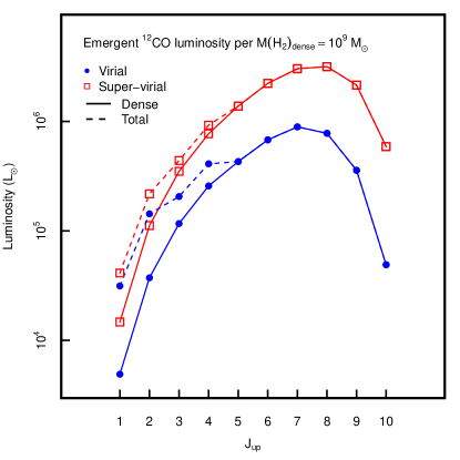
Figure 1.— Emergent ¹²CO spectral line energy distributions for a gas mass of $M_{\rm dense}=10^{9}M_{\odot}$, for our virial ($X_{\rm CO}=9\,M_{\odot}\,{\rm(K\,km\,s^{-1}\,pc^{2})^{-1}}$) and super-virial ($X_{\rm CO}=3\,M_{\odot}\,{\rm(K\,km\,s^{-1}\,pc^{2})^{-1}}$) models. The solid line shows just the emergent flux for the dense phase, and the dashed line shows the total emission when the quiescent (i.e. cold SLED, $X_{\rm CO}=5\,M_{\odot}\,{\rm(K\,km\,s^{-1}\,pc^{2})^{-1}}$) phase is included (see §3.2). This is the most conservative estimate for the molecular line emission from a star-forming galaxy, with the range in CO luminosity given by the two models reflecting the possible range in emission that would arise from different dynamic configurations of the cold ISM in active galaxies (§3.1).

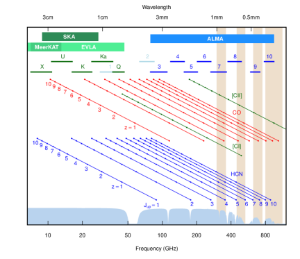
Figure 2.— Schematic view of the visibility of the $J_{\rm up}\leq 10$ transitions of CO and HCN to $z\leq 10$, and the  [C i](${}^{3}P_{1}$$\rightarrow^{3}$$P_{0}$) and [C ii] fine structure lines, indicating the band coverage offered by the SKA high-frequency component and its pathfinder MeerKAT, as well as the radio bands X, U, K, Ka, Q and ALMA Bands 3–10. SKA, MeerKAT and JVLA offers the ability to detect low-J CO and HCN emitting galaxies out to very high redshifts, whereas ALMA covers a broader range of transitions up to high-J over a large span of cosmic time, but can access low-J lines only out to $z\lesssim 3$. The vertical bars show the bandpasses of ground-based instrumentation that could access the FIR lines in the sub-mm regime (e.g. the Redshift and Early Universe Spectrometer [ZEUS], see Stacey et al. 2007).

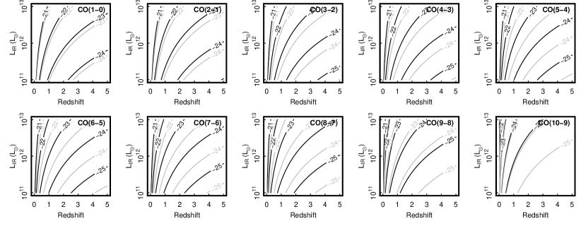
Figure 3.— Predicted CO line fluxes for luminous infrared galaxies as a function of redshift (shown as contours of constant line flux with units of $\log(F/{\rm W\,m^{-2}})$ labelled) from our emergent model. Bold lines show the ‘virial’ model prediction, and grey lines show the equivalent ‘super-virial’ model. Given the sensitivities of submm/mm/cm instrumentation, this model can be used as a conservative estimate of the time required to detect a CO emission line from star-forming (infrared-bright) galaxies across cosmic time. This will be valuable in follow-up spectroscopy of submm continuum surveys to be conducted with, e.g. JCMT, LMT & CCAT that will track LIRG–ULIRG level activity out to $z\sim 5$.

3. The molecular ISM model: a minimalist approach

3.1. The dense, star-forming gas phase

Past studies used rather poorly constrained models of the molecular phase ISM and its CO line excitation range to derive the emergent line luminosities (e.g. Combes et al. 1999; Blain et al. 2000). Here we make use of available HCN $J_{\rm up}\leq 4$ SLEDs of LIRGs (Papadopoulos et al. 2007; Krips et al. 2008; Juneau et al. 2009) to safely extrapolate the corresponding emergent CO SLEDs from  CO J($1$$\rightarrow$$0$) to  CO J($10$$\rightarrow$$9$) for the dense star-forming gas in galaxies. This is possible since even a modestly excited global  HCN J($4$$\rightarrow$$3$) line emission (e.g. HCN $(4\rightarrow 3)/(1\rightarrow 0)=0.30$) implies gas densities $n({\rm H}_{2})\sim 3\times 10^{4}-10^{5}$ cm^-3 (e.g. Papadopoulos et al. 2007), similar to the critical density of  CO J($9$$\rightarrow$$8$) ($n_{\rm cr}$=$2.2\times 10^{5}$$\rm cm^{-3}$). Furthermore, unlike past studies, we use our Large Velocity Gradient (LVG) radiative transfer code to constrain the properties of the dense gas phase using observed global HCN line ratios in LIRGs and $K_{\rm vir}$$\sim$1 where

$$K_{\rm vir}({\rm HCN}) =\frac{\left({\rm d}V/{\rm d}R\right)}{\left({\rm d}V/{\rm d}R\right)_{\rm vir}}$$

$$\sim 1.54\frac{{\rm[HCN/H_{2}]}}{\sqrt{\alpha}\Lambda_{\rm HCN}}\left(\frac{n({\rm H_{2}})}{10^{3}\,{\rm cm}^{-3}}\right)^{-1/2},$$ (1)

parametrizes the average dynamic state of the corresponding gas, with $K_{\rm vir}$$\sim$1 corresponding to virial gas motions (typical for dense HCN-bright star-forming cores in the Galaxy), and $K_{\rm vir}$$\gg$1 corresponding to unbound gas (typically found for low-J CO line emission in LIRGs). The parameter $\alpha\sim 0.55$–$2.4$ depends on the average cloud density profile (see Bryant & Scoville 1996), here we choose $\alpha=1.5$. The quantity $\Lambda_{\rm HCN}={\rm[HCN/H_{2}]}/({\rm d}V/{\rm d}R)$ is one of the three parameters defining the grid of a typical LVG code (the other two being $T_{\rm kin}$ and $n({\rm H}_{2})$). Furthermore we adopt $T_{\rm kin}$$\sim$$T_{\rm dust}$, which is certainly a good approximation for the dense gas phase where strong gas-dust thermal coupling sets in. Abundances of $\rm[HCN/H_{2}]$=$2\times 10^{-8}$ and $\rm[CO/H_{2}]$=10^-4 are adopted for our estimates of $K_{\rm vir}$ for HCN and CO LVG solutions.

Multi-J HCN line surveys of LIRGs find average $r_{J+1,J}({\rm HCN})={\rm HCN}\,(J+1\rightarrow J)/(1\rightarrow 0)$ brightness temperature ratios of $r_{21}{\rm(HCN)}\sim 0.65$ and $r_{32}{\rm(HCN)}\sim 0.45$ (Krips et al. 2008; Juneau et al. 2009). These can be higher still (up to $\sim$1) for extreme mergers whose ISM is dominated by very dense gas (Greve et al. 2009), but the aforementioned ratios are good representatives of the average values observed in LIRGs and we use them as constraints on the properties of the HCN-bright star-forming dense gas phase. The LVG grid is run for temperatures of $T_{\rm kin}=(30-80)$ K fully encompassing the typical range expected for star-forming gas and its concomitant dust. We find $n({\rm H}_{2})=3\times 10^{4}$ cm^-3, $T_{\rm kin}=40$ K, and $K_{\rm vir}\sim 1$ as well as $n({\rm H}_{2})=10^{5}$ cm^-3, $T_{\rm kin}=(30$–$35)$ K and $K_{\rm vir}\sim 8$ as typical solutions. The virial solution is the most likely one for a dense star-forming gas phase in LIRGs (in current turbulence-regulated star-forming models of galaxies self-gravity overcomes turbulent gas motions at such high densities, Krumholz & McKee 2005). We nevertheless consider also the solution with $K_{\rm vir}$$\sim$8, corresponding to gravitationally unbound gas motions; this ‘super-virial’ solution is possibly pertinent to the high density gas found in some extreme starbursts at high redshifts (Swinbank et al. 2011). Any additional excitation mechanisms such as hard X-rays from an active galactic nuclei (AGN; Meijerink & Spaans 2005), and/or high cosmic ray energy densities due to the high supernovae rate densities expected in compact ULIRGs (Papadopoulos 2010) can only raise the dense gas temperatures leading to even more excited HCN and CO SLEDs.

Finally we note that for simplicity we omit the enhanced cosmic microwave background (CMB) as it will have negligible effects on the dense and warm star-forming gas phase in galaxies, even at high redshifts. For a detailed discussion on this see Papadopoulos et al. 2000 (section 4.2), but this can be briefly demonstrated by assuming $T_{\rm kin}=40$ K and $T_{\rm kin}\sim T_{\rm dust}$, typical for the dense, HCN-bright, star-forming gas in LIRGs. The thermodynamically equivalent $T(z)=T_{\rm dust}(z)\sim T_{\rm kin}(z)$ of that phase at $z=5$ would then be: $T(z)={(T(0)^{6}-T_{\rm CMB}(0)^{6}+T_{\rm CMB}(z)^{6})}^{1/6}\approx 40$ K, i.e. it remains essentially identical (a dust emissivity law of $a=2$ is assumed). The impact can be more significant for CO line ratios of a cold and quiescent gas phase (for a $T_{\rm kin}(0)=15$ K, $T_{\rm kin}(z=5)=17.56$ K) where these ratios can be boosted somewhat by the enhanced CMB (see also Table 2 in Papadopoulos et al. 2000), while the line/CMB contrast for the cold, quiescent H₂ phase diminishes. In that regard our assumed local CO line ratios for that phase (see following section) remain conservative and in the spirit of our minimalist approach.

Here we must note that any such global LVG solutions reflect, at best, a rough average of the gas conditions responsible for the observed global line ratios considered. Indeed, as is the case for the so-called $X_{\rm CO}$, $X_{\rm HCN}$, etc. factors that convert the CO and HCN $J=1\rightarrow 0$ line luminosities to mass for the total and the dense molecular gas reservoirs respectively, these LVG solutions represent effective ensemble averages for large collections of molecular clouds, and thus appropriate for unresolved studies of high-$z$ galaxies. In Table 1 we list the LVG-derived line ratios that correspond to the two types of LVG solutions found for the dense gas. These have very similar HCN line ratios up to $J_{\rm up}=5$ (we do not extrapolate above this transition as data for only up to  HCN J($4$$\rightarrow$$3$) exist in the local Universe), and CO up to $J_{\rm up}=4$. Above $J_{\rm up}=4$ we give the range of acceptable values yielded by the LVG model. The corresponding $X_{\rm CO,dense}$ factors are: $\sim$9 $M_{\odot}$ (K km s^-1 pc²)^-1 and $\sim$3 $M_{\odot}$ (K km s^-1 pc²)^-1 for the virial and the super-virial LVG solution respectively, and along with the computed line ratios (Table 1) are used to obtain the range of CO SLEDs for the dense gas shown in Figure 1.

The computed CO SLEDs are minimal in two ways, namely:

1. Only a fraction of the total molecular gas mass in galaxies belongs to this dense star-forming gas phase contributing to such SLEDs at any given moment of their evolution.

2. The observed global HCN line ratios used for their derivation inadvertently include some non-star-forming, less dense gas diluting the HCN ratios from those typical for the star-forming phase alone.

The HCN SLEDs are considered only up to $J_{\rm up}=5$ since: (a) available HCN line data for LIRGs in the local Universe exist only up to $J_{\rm up}=4$ (e.g. Papadopoulos 2007), and (b) only HCN lines up to $J_{\rm up}=3$ were used in our LVG model (thus interpolation beyond $J_{\rm up}=5$ is not safe). We also note that the normalization of the HCN SLED, namely the $X_{\rm HCN}$=$M_{\rm dense}({\rm H_{2}})/L^{\prime}_{\rm HCN}(1\rightarrow 0)$ factor is not identical to that of CO SLEDs since the  HCN J($1$$\rightarrow$$0$) is not fully thermalized (unlike  CO J($1$$\rightarrow$$0$) ) even at the high densities of our LVG solutions. The latter yield $X_{\rm HCN}$={9, 27} $M_{\odot}$ (K km s^-1 pc²)^-1 for the unbound (i.e. super-virial) and the virial solution respectively.

The total CO SLED of a star-forming galaxy will also include non-star-forming gas in a much more tenuous phase. This typically contains the bulk of the molecular gas in individual GMCs, and the molecular gas reservoirs in local LIRGs (except perhaps in ULIRGs). Such quiescent, cool gas at lower densities can thus contribute significantly to the velocity-integrated flux densities of the CO $J_{\rm up}\leq 3$ lines (as well as to the  [C i](${}^{3}P_{1}$$\rightarrow^{3}$$P_{0}$) line of atomic carbon) increasing the source counts in line surveys that would include those transitions. Therefore, in addition to the emergent CO line flux computed for the HCN-bright dense star-forming phase we also include an estimate for the low-J CO emission from this cold, quiescent phase.

3.2. The cold, quiescent gas phase

In the local Universe the star formation ‘mode’ seems to be very well (i.e. uniquely) indicated by the fraction of the total gas reservoir residing in the dense phase: $\xi_{\rm SF}=M_{\rm dense}(\rm H_{2})/M_{\rm tot}(\rm H_{2})$. Local studies suggest typical values of $\xi_{\rm SF}\sim 0.25$ (and even $\gtrsim$0.50) for merger-driven starburst systems (Solomon et al. 1992a; Gao & Solomon 2004; Papadopoulos et al. 2012) and $\xi_{\rm SF}\sim 0.025$ for secular activity in ‘quiescent’ systems, with the complete star-forming population potentially forming a continuum of $\xi_{\rm SF}$ (cf. Daddi et al. 2010). Therefore, an estimate of the mass of the quiescent, non-star-forming gas phase can be calculated by:

$$M_{\rm quiescent}({\rm H_{2}})=M_{\rm dense}({\rm H_{2}})\left(\frac{1-\xi_{\rm SF}}{\xi_{\rm SF}}\right)$$ (2)

In the spirit of our ‘minimal’ approach, the most conservative estimate of $M_{\rm quiescent}(\rm H_{2})$ is given by assuming all galaxies are in the burst mode, with $\xi_{\rm SF}=0.25$, such that $M_{\rm quiescent}({\rm H_{2}})=3\times M_{{\rm dense}}({\rm H_{2}})$. Armed with this mass estimate, we can assign CO luminosities by assuming a fixed, representative SLED for this phase.

We assume the ‘coldest’ known CO SLED in the local Universe, which is found in cold quiescent clouds in M 31 with CO line ratios: $r_{\rm 21}=0.42\pm 0.10$, $r_{\rm 32}=0.14\pm 0.04$, $R_{\rm 12/13}{\,J(1\rightarrow 0)}={\rm{}^{12}CO/^{13}CO}=9\pm 2$ (Allen et al. 1995; Loinard et al. 1995, 1996; Loinard & Allen 1998; Israel et al. 1998 and references therein). For the  [C i](${}^{3}P_{1}$$\rightarrow^{3}$$P_{0}$) line emission in the same environments $r_{\rm[CI]/CO}{\rm(1-0)}=0.1\pm 0.02$ (Wilson 1997; Israel et al. 1998), while COBE determined the [CI]($2\rightarrow 1$)/($1\rightarrow 0$) line ratio (difficult to obtain from the ground) in the similar environment of the outer Galaxy disk to be $r_{\rm[CI]}(2\rightarrow 1/1\rightarrow 0)=0.22\pm 0.09$ (Fixsen et al. 1999). We then use our LVG radiative transfer model, constrained by the available CO, ¹³CO line ratios and $K_{\rm vir}$$\sim$1 to find the corresponding average ISM states, higher-J CO line luminosities, and compute the $X_{\rm CO}$ factor normalizing the cold CO SLED in terms of H₂ molecular gas mass. We find typical virial LVG solutions with $T_{\rm kin}=(10-15)$ K, and $X_{\rm CO}$$\sim$5 $M_{\odot}$(K km s^-1 pc²)^-1 (i.e. typical of cold GMCs in the Galaxy) and CO line ratios of $r_{\rm 21}=0.45$–$0.55$, $r_{\rm 32}=0.12-0.13$, $r_{\rm 43}=0.09-0.011$ and $r_{\rm(J+1)-J}$$\lesssim$$10^{-4}$ for $(J+1)$$>$4. We plot the additional cold component of the quiescent gas phase in Figure 1. In Figure 2 we present a schematic plot indicating the observed frequency and atmospheric windows of the principle emission lines we consider in this work.

3.3. Far-infrared cooling lines

The dominant coolant for the warm ($T<1000$ K) neutral ISM is the far-infrared (FIR) fine structure line [Cii] 158$\mu$m, carrying up to 1% of the total FIR output. When redshifted beyond $z>1$ this line will be an important contributor to detections in the submillimeter bands, and therefore important to consider in our model.

We adopt an semi-empirical prescription for estimating the luminosity of [C ii] based on the compendium of Infrared Space Observatory (ISO) Long Wavelength Spectrometer (LWS) observations of 227 local ($cz\lesssim 10^{4}$ km s^-1) galaxies by Brauher, Dale & Helou (2008). These authors note the scalings between the principle FIR fine structure line luminosities and FIR luminosity (here we consider the IRAS FIR luminosity to be equivalent to our assumed total infrared luminosity) of galaxies, as well as the far-infrared color $f_{60}/f_{100}$ (sensitive to the intensity of the underlying radiation field heating the dust; Stacey et al. 2010). For example, the ratio $L_{\rm[CII]}/L_{\rm FIR}$ drops from 1% to 0.1% with increasing (hotter) $f_{60}/f_{100}$ . This could reflect a harder and more intense far-UV field that results in conditions less efficient at producing C⁺ (Malhotra et al. 2001), or an extra contribution to the FIR continuum from regions not associated with the PDRs (Luhman et al. 2003; Stacey et al. 2010). This phenomenon has become known as the [Cii] deficit, although it is not clear whether it is a true deficit.

To evaluate the relevant scalings between line luminosities and IR luminosity, we only consider galaxies in the Brauher, Dale & Helou compendium with nuclear regions classed as ‘star-forming’ that were unresolved by the LWS beam (D. Dale, private communication). Fitting a linear trend to the data, we find the scaling:

$$\log\left(L_{\rm[CII]}/L_{\rm FIR}\right)=(-0.74\pm 0.39)\left(f_{60}/f_{100}\right)-(2.08\pm 0.25).$$ (3)

The uncertainties are the 1$\sigma$ errors in the formal fit and reflect the large scatter in the data. Although the strength of the [C ii] line varies by a factor $\sim$10, and can contribute up to $\sim$1% of the FIR luminosity, in the spirit of our minimalist approach, we adopt a conservative scaling that predicts a modest emergent $L_{\rm[CII]}$ for a galaxy with $L_{\rm IR}$. We therefore adopt $f_{60}/f_{100}$ $=1$, which yields $\log\left(L_{\rm[CII]}/L_{\rm FIR}\right)={-2.8}$. While this value is a conservative estimate for local galaxies, is it appropriate for (on average higher luminosity) high-redshift star-forming populations? Given the high luminosity of the line, there is a growing sample of [C ii] detections in ULIRG-class systems. For example, Stacey et al. (2010) find a an average ratio of $\log\left(L_{\rm[CII]}/L_{\rm FIR}\right)=-2.5$ for (star formation dominated) ULIRGs at $1\lesssim z\lesssim 2$; we therefore consider our canonical value based on the extreme tail of local star-forming galaxies suitable for application in our model.

3.3.1 The [C ii] line as tracer of CO-dark H₂ at high redshifts

The presence of a CO-deficient and even CO-dark molecular gas reservoir is expected in globally metal-poor systems such as local dwarf galaxies as well as Lyman-break galaxies (LBGs) at high redshifts, the result of efficient CO dissociation and a strongly self-shielding H₂ (e.g. Pak et al. 1998). Such a phase is even expected in typical local spiral disks at large galactocentric distances as a result of metallicity gradients (Papadopoulos et al. 2002). This very much inhibits the detection of such H₂ gas reservoirs via the workhorse CO lines but at the same time anticipates very bright [C ii] emission. In local dwarf galaxies the latter revealed $\sim$10–100 times larger molecular gas mass than that inferred by CO (Madden et al. 1997).

Similarly strong [C ii] emission is expected for high-z systems like LBGs which are very difficult to detect in CO lines (see Baker et al. 2004, Coppin et al. 2007 for the only such examples), while early evidence seems to corroborate this for other types of high-z systems (Maiolino et al. 2009). A general [C ii] emission enhancement at high redshifts with respect to that expected from local template systems with similar infrared luminosities can be a result of a general evolutionary trend towards more metal-poor gas reservoirs at earlier epochs, and could much enhance the potential of the [C ii] as a galaxy redshift survey tool. We caution though that its emission, once detected, will be much harder than, for example,  [C i](${}^{3}P_{1}$$\rightarrow^{3}$$P_{0}$) to interpret solely in terms of total molecular gas mass as the [C ii] line will contain significant contributions from ionized and neutral hydrogen (e.g. Madden et al. 1997). These non-H₂ contributions to [C ii] line emission will be hard to correct for at high redshifts, where they may actually be boosted in metal-poor environments and/or strong average far-UV radiation fields of nascent starbursts.

To explore these possibilities we assume a population of objects with $L_{\rm[CII]}/L_{\rm IR}=10^{-2}$, a value typical for the LMC and IC 10 (Madden et al. 1997). At such levels the [C ii] line of LIRG-class systems can be detected right out to the epoch of re-ionisation ($z\sim 10$) with ALMA in bands 4–9, within 8 hrs of full aperture synthesis observations (assuming one bin channel of 300 km s^-1, see §5.1). The evolutionary track of the SFR of such a putative galaxy population with a nearly CO-dark ISM is unknown, leaving the line number counts uncertain, however we discuss the potential for blind discovery of such systems assuming their abundance and evolution is identical to that of LBGs in §5.1.1.

3.4. Calculating line luminosities

For the various computations and transformations between line luminosity types, and for linking the latter to observed velocity-integrated line fluxes we use standard relations,

$$L^{\prime}_{x} =\int_{\Delta V}\int_{A_{s}}T_{b,x}\,da\,dV$$

$$=\frac{c^{2}}{2k_{B}\nu^{2}_{\rm x,rest}}\left(\frac{D^{2}_{L}}{1+z}\right)\int_{\Delta V}S_{\nu}\,dV,$$ (4)

where $T_{\rm b,x}$ is the rest-frame brightness temperature of the line, $\Delta V$, $A_{\rm s}$ are the line FWZI and source area respectively. After substituting astrophysical units this yields,

$$L^{\prime}_{x}=3.25\times 10^{7} \left[\frac{D^{2}_{L}({\rm Mpc})}{1+z}\right]\left(\frac{\nu_{\rm x,rest}}{\rm GHz}\right)^{-2}$$

$$\times\left[\frac{\int_{\Delta V}S_{\nu}\,dV}{\rm Jy\,km\,s^{-1}}\right]\,{\rm K\,km\,s^{-1}\,pc^{2}},$$ (5)

where $D_{L}$ is the luminosity distance, and $\nu_{\rm x,rest}$ is the rest frame line frequency. The conversion to traditional luminosity units ($L_{\odot}$), used for the total line luminosities ($L_{x}$=$\int L_{\nu}\,d\nu$) in CO SLEDs, can be made using

$$L_{x} =\frac{8\pi k_{B}\nu^{3}_{\rm x,rest}}{c^{3}}\,L^{\prime}_{x}$$

$$=3.18\times 10^{4}\left(\frac{\nu_{\rm x,rest}}{\rm 100\,GHz}\right)^{3}\left[\frac{L^{\prime}_{x}}{10^{9}\,{\rm K\,km\,s^{-1}\,pc}^{2}}\right]L_{\odot}.$$ (6)

Note that integrated line fluxes are related to the commonly used $S\Delta V$ integrated flux density units by:

$$\left(\frac{3\times 10^{-4}}{\nu_{\rm obs}\,\,{\rm GHz}}\right)\times\left(\frac{F}{{\rm 10^{-26}\,W\,m^{-2}}}\right)=\left(\frac{S\Delta V}{\rm Jy\,km\,s^{-1}}\right).$$ (7)

Table 1Normalized emergent CO and HCN SLEDs

Transition		$r_{\rm J+1,J}$a
		CO (dense)	CO (quiescent)	HCN
1$\rightarrow$	0	1.00	1.00	1.00
2$\rightarrow$	1	0.95	0.50	0.75
3$\rightarrow$	2	0.88	0.13	0.40
4$\rightarrow$	3	0.82	0.09	0.15
5$\rightarrow$	4	0.70–0.75	10-4	0.05
6$\rightarrow$	5	0.64–0.70
7$\rightarrow$	6	0.53–0.60
8$\rightarrow$	7	0.31–0.42
9$\rightarrow$	8	0.10–0.20
10$\rightarrow$	9	0.01–0.04
a$r_{\rm J+1,J}=L^{\prime}_{{\rm J+1\rightarrow J}}/L^{\prime}_{{\rm 1\rightarrow 0}}$

3.5. The normalization of dense molecular gas SLEDs

The final remaining step for calculating the emergent molecular line emission from a star-forming galaxy is to normalize the SLEDs according to the infrared luminosity (i.e. SFR) of the system. Recent studies of star formation feedback suggest a maximum $\epsilon_{\star}=L_{\rm IR}/M_{\rm dense}({\rm H}_{2})\sim 500$ $(L_{\odot}/M_{\odot})$ for the dense and warm gas $M_{\rm dense}({\rm H}_{2})$ near star forming sites in galaxies as a result of strong radiation pressure from the nascent O, B star clusters onto the concomitant dust of the accreted gas fuelling these sites (Scoville 2004; Thompson et al. 2005; Thompson 2009). Thus, provided that average dust properties (e.g. its effective radiative absorption coefficient per unit mass) remain similar in metal-rich star-forming systems such as LIRGs, a near-constant $\epsilon_{\star}$ is expected for the dense star-forming gas. A value of $\epsilon_{\star}\sim 500$ $(L_{\odot}/M_{\odot})$ is actually measured in individual star-forming sites of spiral disks such as M 51 and entire starbursts such as Arp 220 (Scoville 2004), while $\sim$($440\pm 100$) $(L_{\odot}/M_{\odot})$ is obtained for CS-bright star-forming cores in the Galaxy (Shirley et al. 2003). It must be noted however that the intermittency expected for galaxy-sized molecular gas reservoirs (i.e. at any given epoch of a galaxy’s evolution some dense gas regions will be forming stars while others will not) can lower the global $\epsilon_{\star}$ to $\sim$$\nicefrac{{1}}{{3}}$–$\nicefrac{{1}}{{2}}$ of the Eddington value (Andrews & Thompson 2011).

Similar $\epsilon_{\star}$ values can be obtained without explicit use of the Eddington limit (and the detailed dust properties it entails), but from the typical $L_{\star}/M_{\rm new,\star}$ in young starbursts where $M_{\rm new,\star}$ is the mass of the new stars and $L_{\star}$ their bolometric luminosity ($\sim$$L_{\rm IR}$ for the deeply dust-enshrouded star-forming sites). For $\epsilon_{\rm SF,c}$=$M_{\rm new,\star}/[M_{\rm new,\star}+M_{\star}({\rm H}_{2})]$ as the star formation efficiency (SFE) of the dense gas regions where the new stars form is:

$$\epsilon_{\star}=\frac{\epsilon_{\rm SF,c}}{1-\epsilon_{\rm SF,c}}\left(\frac{L_{\rm IR}}{M_{\rm new,\star}}\right).$$ (8)

For $\epsilon_{\rm SF,c}$$\sim$0.3–0.5 typical for dense star-forming regions, and $L_{\rm IR}/M_{\rm new,\star}=$300–400 $(M_{\odot}/L_{\odot})$ (Downes & Solomon 1998 and references therein), equation 8 yields $\epsilon_{\star}$$\sim$130–400 $(M_{\odot}/L_{\odot})$. Here we choose $\epsilon_{\star}=$250 $(L_{\odot}/M_{\odot})$, close to the average values yielded by equation 8, and the black body limit deduced for the compact CO line emission concomitant with an optically thick ($\tau_{\rm 100\,\mu m}$$>$1) dust emission seen in ULIRGs (Solomon et al. 1997).

Thus Eddington-limited (i.e. radiation pressure limited) star formation in LIRGs sets a near-constant mass normalization of the dense star-forming gas phase using the star formation driven infrared luminosity and thus allows a $M_{\rm dense}({\rm H}_{2})$/SFR value to be deduced. This can then be used to set the absolute scale of the emergent minimal CO SLEDs of the star-forming gas phase using the SFR($z$) of an input galaxy evolution model, since it is

$$L^{\prime}_{\rm CO}(1-0) =M_{\rm dense}({\rm H_{2}})/X_{\rm CO}$$

$$=L_{\rm IR}/\epsilon_{*}X_{\rm CO}$$

$$=k_{\rm sfr}{\rm SFR}/\epsilon_{*}X_{\rm CO}$$ (9)

which can be converted to solar units using equation 6, and with an identical relation applying to the  HCN J($1$$\rightarrow$$0$) line luminosity but utilizing the corresponding $X_{\rm HCN}$ values.

In Figure 3 we present the observed CO line fluxes predicted for both the virial and super-virial models for a range of $L_{\rm IR}$ and redshift; this can be used as a ‘ready reckoner’ to estimate the CO line flux for a given galaxy where some estimate of the infrared luminosity is known. As noted in §3.1, the LVG solutions for the dense gas phase are $X_{\rm CO}$={3, 9} $M_{\odot}$(K km s^-1 pc²)^-1, and $X_{\rm HCN}$={9, 27} $M_{\odot}$(K km s^-1 pc²)^-1 for the super-virial and virial cases. Given the well-excited CO SLEDs expected for the dense star-forming gas phase (Figure 1), their normalization to the dense gas mass, namely the $X_{\rm CO}$ factor, determines to a great degree the ‘visibility’ of these SLEDs in the distant Universe. For a given amount of dense gas lower $X_{\rm CO}$, $X_{\rm HCN}$ values than the adopted ones correspond to brighter CO and HCN SLEDs though we consider them unlikely for the self-gravitating or only modestly unbound dense star-forming gas in LIRGs.

The LVG-derived CO line ratios (Table 1) can then be used to derive the expected fluxes for the other CO transitions from the SFR-normalized $L^{\prime}_{\rm CO(1-0)}$. For systems with lower metallicities we assume proportionally less dust per molecular gas, and thus the Eddington limit becomes $\epsilon_{\star}=250(Z/Z_{\odot})^{-1}$ $(L_{\odot}/M_{\odot})$, where $Z$ is the metallicity. Finally we note that while the dense HCN-bright gas fuelling star formation will be often a small fraction of the total molecular gas mass in galaxies it is nevertheless the only phase for which the frequently-used gas consumption timescale $\tau_{\rm cons}$=$M_{\rm dense}({\rm H}_{2})$/SFR may have its intended physical meaning as the duration of an observed star formation event. Strong star-formation and/or AGN feedback will almost certainly modify the ‘consumption’ timescale especially for the extended, less dense, quiescent molecular gas by inducing powerful outflows (Sakamoto et al. 2009; Feruglio et al. 2010; Chung et al. 2011), or by fully dissociating large fractions of H₂ gas mass towards warmer and diffuse phases unsuitable for star formation such as Cold Neutral Medium (CNM) and Warm Neutral Medium (WNM) Hi gas (Pelupessy et al. 2006).

Lower metallicities will not have any effect on the emergent CO SLED shapes of the dense star forming gas phase in galaxies as long as the optical depths of the CO lines remain significant. Nevertheless the CO-bright part of individual H₂ clouds will shrink, leaving behind [C ii] and  [C i](${}^{3}P_{1}$$\rightarrow^{3}$$P_{0}$) bright H₂ gas (Bolatto et al. 1999 [Figure 1]; Pak et al. 1998). Thus the expected first order effect of lower metallicities would be to lower all CO line luminosities per H₂ mass, while boosting up the [C ii] and  [C i](${}^{3}P_{1}$$\rightarrow^{3}$$P_{0}$) line luminosities. The latter may be crucial in the detection of metal-poor galaxies at high redshifts (see section 3.3.1).

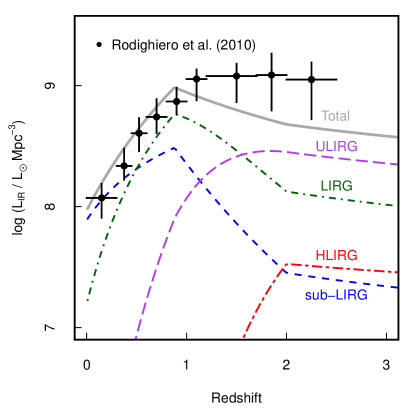
Figure 4.— Model of the evolution of the infrared luminosity density, figure adapted from Figure 12 of Béthermin et al. (2011). Breaking down the total contribution into sub-LIRG ($L_{\rm IR}<10^{11}L_{\odot}$), LIRG ($L_{\rm IR}=10^{11-12}L_{\odot}$), ULIRG ($L_{\rm IR}=10^{12-13}L_{\odot}$) and HLIRG ($L_{\rm IR}>10^{13}L_{\odot}$) clearly shows how the dominance changes from low-luminosity spiral galaxies in the local Universe, through LIRGs at the peak of the luminosity density and to ULIRGs at $z>2$. We use the model of Béthermin et al. as a basis for predicting the number density of star-forming galaxies across cosmic time. The points show the measurements of Rodighiero et al. (2010) which are based on Herschel PACS observations of the GOODS-N field. This figure also illustrates the basic form of the model: rapid evolution in both space density and characteristic luminosity to $z\sim 0.9$, followed by two phases of negative evolution to high-z.

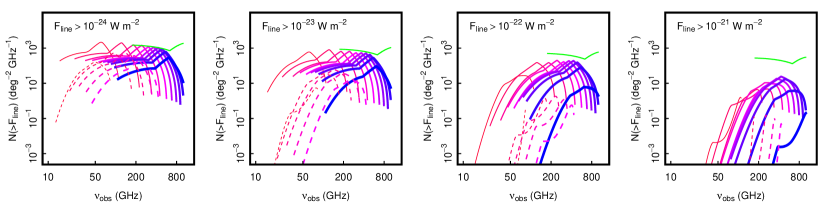
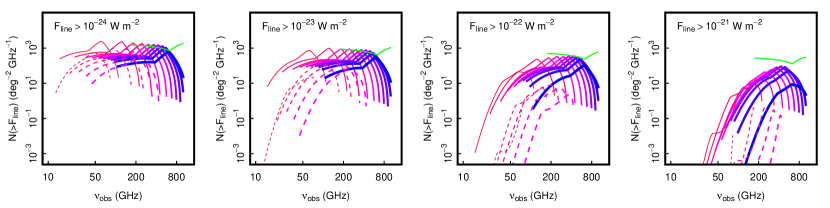
Figure 5.— Counts of galaxies with CO $J_{\rm up}\leq 10$ (solid lines, blue/thick to red/thin for increasing J), HCN $J_{\rm up}\leq 5$ (dashed lines blue/thick to red/thin for increasing J), [C ii] (green line) and $F_{\rm line}$$>$$10^{-24}$–$10^{-21}$ W m^-2 as a function of observing frequency for the virial (top row) and super-virial SLED models (bottom row). We calculated the integrated counts for each line in a sliding 8 GHz wide window, and therefore quote the counts as the average per unit bandpass. The sharp cut-offs at the highest frequencies of each line correspond to $z=0$, and the predictions terminate at frequencies corresponding to $z=10$ in this figure. The distinctive shape of the counts when presented in this way is simply a reflection of the form of the evolution of the IR luminosity function, which has a peak of activity at $z\sim 1$–$2$, followed by weak negative evolution to high-$z$ (see §4).

3.6.  [C i](${}^{3}P_{1}$$\rightarrow^{3}$$P_{0}$) and HCN lines: a new promising avenue towards total gas mass and the star formation mode

The submillimeter lines of atomic carbon, and especially  [C i](${}^{3}P_{1}$$\rightarrow^{3}$$P_{0}$) at 492 GHz have been proposed as powerful alternatives to the  CO J($1$$\rightarrow$$0$) or  CO J($2$$\rightarrow$$1$) lines as total molecular gas mass tracers (Papadopoulos et al. 2004), and have been shown to work to that effect in local LIRGs (Papadopoulos & Greve 2004). The  [C i](${}^{3}P_{1}$$\rightarrow^{3}$$P_{0}$) line may actually be a better tracer of total molecular gas mass than  CO J($1$$\rightarrow$$0$) (Papadopoulos et al. 2004), taking advantage of the positive k-correction with respect to the  CO J($1$$\rightarrow$$0$) line (while the  CO J($4$$\rightarrow$$3$) line at similar frequency to  [C i](${}^{3}P_{1}$$\rightarrow^{3}$$P_{0}$) is a poor total molecular gas mass tracer as it is tied to the star-forming gas phase). Moreover  [C i](${}^{3}P_{1}$$\rightarrow^{3}$$P_{0}$) is optically thin (thus it does not need ‘$X$’ factors to trace mass), has a simple partition function, is easily excitable for the bulk of the H₂ gas mass in galaxies, and of course remains accessible to ALMA for a much wider range of redshifts than  CO J($1$$\rightarrow$$0$) or  CO J($2$$\rightarrow$$1$) (Figure 2). When combined with a tracer of the dense, star-forming gas phase, combinations of, e.g.  HCN J($1$$\rightarrow$$0$) and  [C i](${}^{3}P_{1}$$\rightarrow^{3}$$P_{0}$) could be a powerful tracer of the star formation ‘mode’ of a galaxy, as traced by $M_{\rm dense}({\rm H}_{2})/M_{\rm total}({\rm H}_{2})$. We discuss the prospect of practical surveys of the star formation mode in an accompanying Paper II (Papadopoulos & Geach 2012).

4. Galaxy number counts model

In order to use the line emission model to predict the number counts in a blind molecular line survey, we require a framework for the evolution of the abundance of galaxies as a function of infrared luminosities (i.e. the SFR history traced by the evolution of the infrared luminosity density). This can then be used to derive the corresponding evolution of $M_{\rm dense}({\rm H_{2}})$, and thus the emergent molecular line emission.

We use the ‘backwards evolution’ parametric model of Béthermin et al. (2011), which is a phenomenological model of the evolution of the bolometric luminosity function, based on the philosophy of Lagache et al. (2003), but updated to fit the latest empirical results from large area infrared and sub-mm surveys, including recent results from Herschel. Béthermin et al. (2011) employ a three-step evolution of the IR luminosity function, which evolves as $(1+z)^{Q}$ in $\phi_{\star}$ and $L_{\star}$, with two redshift breaks (at $z=0.89$ and $z=2$) where the exponents of the evolution coefficients change. In summary, the model can be described as a steep rise in the IR luminosity density out to the first break, followed by a rapid negative evolution to $z=2$ (i.e. there is a ‘burst’ of activity at $z\sim 1$–$2$), followed by weak negative evolution to high-$z$. The model is only empirically constrained to $z\sim 3$, and so we caution the reader that extrapolations to higher redshifts, as we present here, are inherently uncertain. We examine the impact of an order-of-magnitude change in the infrared luminosity density evolution at $z>3$ on our predicted counts in §5.1.1, and we acknowledge that any predictions we make for the abundance of gas reservoirs at very high redshifts are rather speculative; this was, in part, our motivation for a ‘minimal’ ISM model for the number counts.

The infrared luminosity density evolution model is successful at re-producing the differential counts across the full range of typical bandpasses, 24–850$\mu$m, as well as the observed evolution of the infrared luminosity function. The evolution of the infrared luminosity density broken into contributions from sub-LIRG ($L_{\rm IR}<10^{11}L_{\odot}$), LIRG ($L_{\rm IR}=10^{11-12}L_{\odot}$), ULIRG ($L_{\rm IR}=10^{12-13}L_{\odot}$) and HLIRG ($L_{\rm IR}>10^{13}L_{\odot}$) classes is shown in Figure 4, compared to the latest measurements of the total infrared luminosity density from Herschel (Rodighiero et al. 2010). Beyond $z\sim 1$ the model slightly under-predicts the luminosity density (although the observational constraints become more uncertain at this epoch), indicating that the model could be considered a conservative estimate of the galaxy counts at high-$z$.

Table 2Predicted number counts of molecular emission lines

Band	$\nu_{\rm obs}$	FoVa		rmsc	$\log F_{\rm 1\,hour}$	$\log F_{\rm opt}$	$N(>$$F_{\rm 1\,hour})$	$N(>$$F_{\rm opt})$	1hr rate		Optimal rate		Serendipitous
	GHz	arcmin2		$\mu$Jy $\surd$hr	W m-2	W m-2	deg-2	deg-2	hour-1		hour-1		10 hre
Virial SLED model
MeerKATb	10	55.	44	38	$-$22.7	$-$23.4	$<$1	92	0.	011	0.	046	0.39
SKA Kb	18	11.	16	1	$-$23.8	$-$22.8	2215	122	6.	867	35.	282	14.93
ALMA Band 3	103	0.	83	77	$-$21.4	$-$21.5	174	231	0.	040	0.	041	0.28
ALMA Band 4	147	0.	40	77	$-$21.2	$-$20.0	629	33	0.	070	1.	099	0.24
ALMA Band 5	163	0.	24	86	$-$21.2	$-$20.0	761	69	0.	050	0.	881	0.15
ALMA Band 6	212	0.	14	75	$-$21.1	$-$21.1	946	1033	0.	037	0.	034	0.10
ALMA Band 7	278	0.	08	87	$-$20.9	$-$21.0	911	1137	0.	020	0.	015	0.05
ALMA Band 8	406	0.	04	288	$-$20.2	$-$21.0	383	1216	…		…		…
ALMA Band 9	668	0.	02	721	$-$19.6	$-$21.0	265	1026	…		…		…
ALMA Band 10	854	0.	01	1526	$-$19.2	$-$20.0	357	922	…		…		…
Super-virial SLED model
MeerKATb	10	55.	44	38	$-$22.7	$-$23.3	1	91	0.	029	0.	079	0.75
SKA Kb	18	11.	16	1	$-$23.8	$-$22.7	3164	135	9.	811	70.	894	21.34
ALMA Band 3	103	0.	83	77	$-$21.4	$-$20.1	623	$<$1	0.	144	0.	040	0.66
ALMA Band 4	147	0.	40	77	$-$21.2	$-$20.0	1341	34	0.	150	1.	122	0.46
ALMA Band 5	163	0.	24	86	$-$21.2	$-$20.0	1730	74	0.	115	0.	946	0.31
ALMA Band 6	212	0.	14	75	$-$21.1	$-$20.5	2195	483	0.	086	0.	336	0.20
ALMA Band 7	278	0.	08	87	$-$20.9	$-$20.3	2176	576	0.	048	0.	181	0.11
ALMA Band 8	406	0.	04	288	$-$20.2	$-$20.3	615	703	0.	007	0.	006	0.02
ALMA Band 9	668	0.	02	721	$-$19.6	$-$20.2	283	566	…		…		…
ALMA Band 10	854	0.	01	1526	$-$19.2	$-$20.0	359	940	…		…		…
aassuming field-of-view is equivalent to full width at half maximum of primary beam
bcounts per 4 GHz window
c1$\sigma$ noise in 300 km s-1 channel
dtime required to detect integrated 300 km s-1 line at 5$\sigma$
enumber of sources detected at $>$5$\sigma$ in 300 km s-1 channels in a 10 hour integration, per field-of-view in a 4 or 8 GHz bandwidth
‘…’ indicate the counts are effectively zero for practical purposes ($<$$10^{-3}$ hr-1)

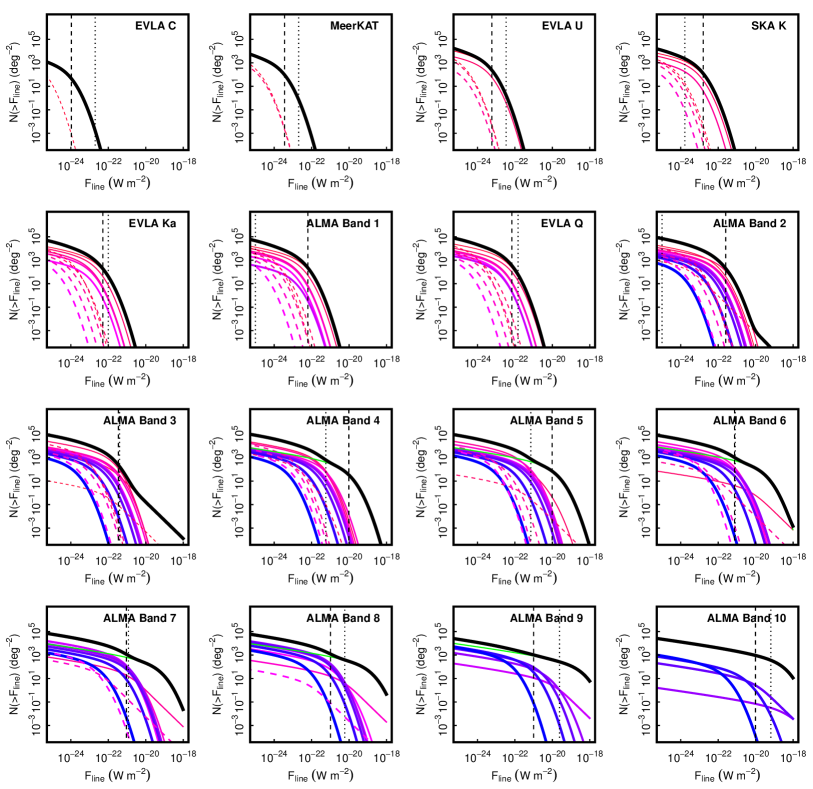
Figure 6.— Integrated number counts in our virial SLED model of CO $J_{\rm up}\leq 10$, HCN $J_{\rm up}\leq 5$ and [C ii] lines in 8 GHz wide bands at the central frequencies of the submm–cm bands (although Bands 1 and 2 are currently hypothetical, pending development). The dashed vertical line indicates where the slope of the counts rolls through $N\propto F^{-2}$, thus indicating the flux limit corresponding to an ‘optimal’ survey at a given frequency (Blain et al. 2000) and the vertical dotted line indicates the 5$\sigma$ depth for a 1 hour integration (this is unknown for ALMA Band 1 and 2).

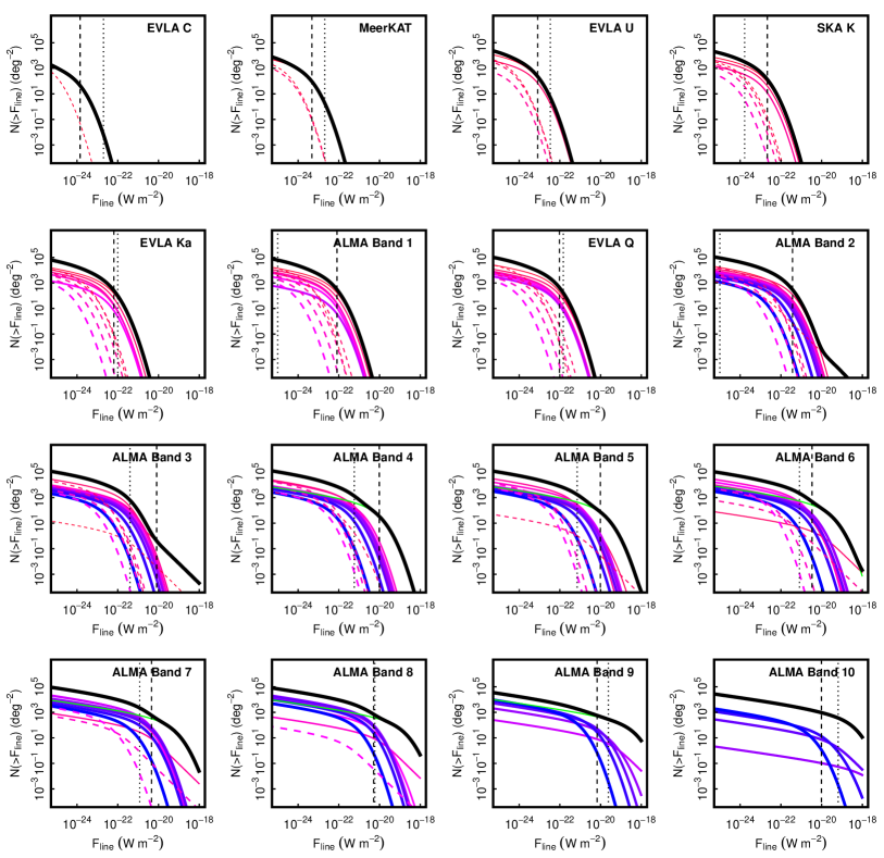
Figure 7.— Integrated number counts in our super-virial SLED model, caption as Figure 6.

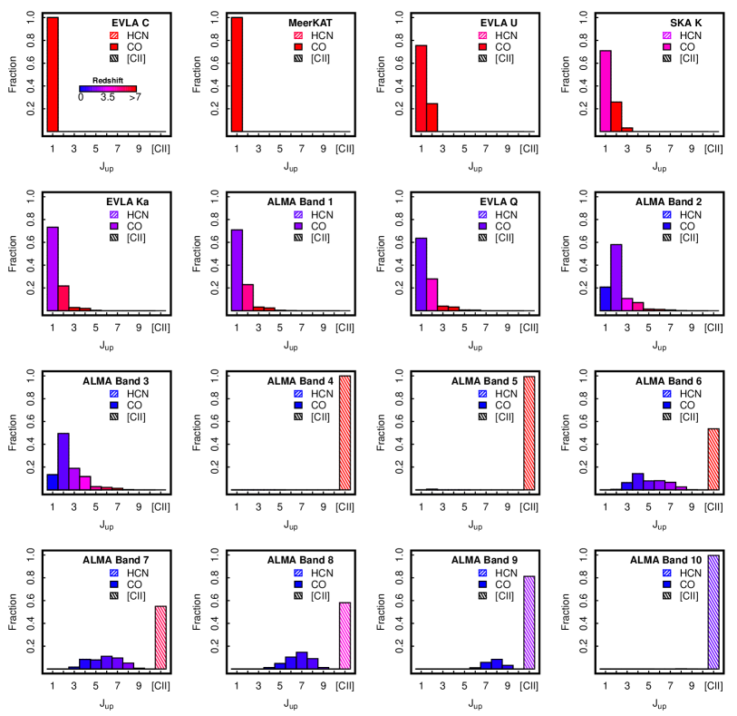
Figure 8.— Break-down of line species detected at the optimal flux limit of each band in the virial model (Fig. 6). Bars are colored by the average redshift of each line, clearly indicating the transition from the dominance of low-J/high-z detections at low frequencies (accessible with MeerKAT, JVLA and MeerKAT, etc.) through a more diverse yield of mid-J/medium-z lines and [C ii] dominance in the ALMA bands. HCN emitters always represent a tiny fraction of detections in optimal surveys.

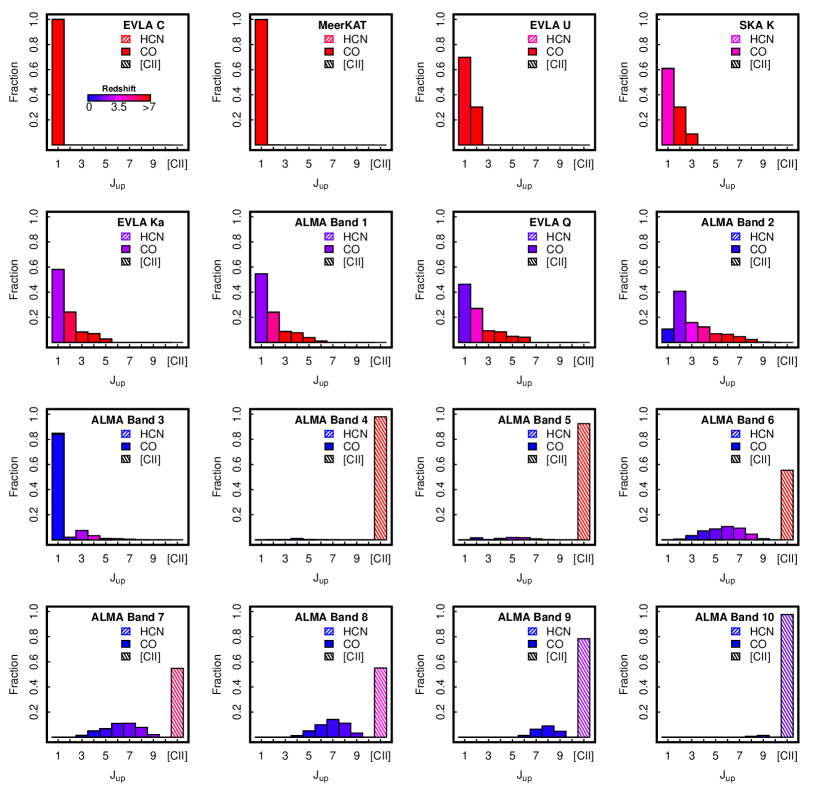
Figure 9.— Break-down of line species detected at the optimal flux limit of each band in the super-virial model (Fig. 7). Caption as Figure 8.

5. Results

5.1. Minimal integral number counts in a line flux limited survey

The model of infrared number counts provides the framework on which to predict the number counts of molecular lines emitted by star-forming galaxies, since $L_{\rm IR}\propto M_{\rm dense}({\rm H_{2}})$. We apply the minimal emergent model of CO emission presented in §3 to predict $L_{\rm IR}$ for a given line of integrated flux $F_{\rm line}$ seen at observed frequency $\nu_{\rm obs}$. The $L_{\rm IR}(z)$ model can then be integrated to predict the lower limit to the number counts of objects detected in a line flux limited survey across the full mm–cm regime.

In Figure 5 we plot the minimal number counts across $20<\nu_{\rm obs}<1200$ GHz for [C ii] , HCN and CO $J_{\rm up}\leq 10$ line emitting galaxies with $F_{\rm line}>10^{-24}$–$10^{-21}$ W m^-2, averaged over an 8 GHz sliding window. Care will have to be taken to correctly identify single lines; the most robust strategy would be to detect two or more molecular lines for an accurate redshift identification. The shape of the counts of the individual lines reflects the evolution of the underlying luminosity density described in §4.

This burst of activity at $z\sim 1$ results in a corresponding peak in the line counts, which is probably artificially sharp in the present model; in reality we might expect a smoother turn-over (this can be mimicked by averaging the counts over a wider bandwidth). Nevertheless, this demonstrates the power a molecular line survey could have as a probe of the evolution of the galaxy population, as the yield of line emitters in a spectral survey over sufficiently wide frequency range ($>$100 GHz) will be a clean and sensitive tracer of the history of galaxy evolution that is complementary to previous studies that have focused on the evolution of the SFR and stellar mass functions.

It will not be possible to fully sample the frequency range shown in Figure 2. Line searches from the ground are strictly restricted to the frequency windows dictated by the atmospheric transmission (the most significant for evolutionary surveys being the telluric feature at $\sim$60 GHz), and the availability of receivers capable of detecting the radiation transmitted through such windows. In the following sections we examine the number counts expected in practical blind surveys conducted by the latest arrays with the sensitivity capable of performing them: ALMA, SKA and its pathfinder MeerKAT. JVLA will not be powerful enough to perform a blind survey, although we examine the number counts in the standard radio bands. We consider the detection-rate of molecular emission lines in two types of observing campaigns:

1. Individual pointings of one hour integrations searching for $\geq 5\sigma$ detections of lines in 300 km s^-1 ($\Delta\nu=\nu/10^{3}$ GHz) bins (i.e. an integrated line detection where information about the line profile is discarded) across a set bandwidth. This strategy could be used for a controlled (i.e. flux limited) survey for a particular line species.

2. Individual pointings that reach a line flux limit corresponding to the the knee of the integrated counts where $N(>F)\propto F^{-2}$, thus optimizing the detection rate of sources for a fixed observing time, again for detections in 300 km s^-1 channels (see Blain et al. 2000 and Carilli & Blain 2002). This strategy could be used for a simple ‘redshift search’, where one aims to simply identify large numbers of galaxies at high-$z$, or identify unique classes of object that are unlikely to be found by any other means.

We note that that may be other routes to blind redshift surveys; for example, sensitive Fourier Transform Spectrometers (FTSs) that take advantage of the large fields of view of future submm telecopes (e.g. CCAT potentially has a usable field-of-view of 1^∘). These could also be used for blind tomographic surveys of [C ii] in the submm atmospheric windows (Figure 2) in a similar manner to narrowband surveys of emission line galaxies in the OIR bands.

5.1.1 Atacama Large Millimeter Array

ALMA covers the frequency range 80–900 GHz, which will possibly be extended down to 40 GHz with the addition of Bands 1 and 2, which would allow coverage of low-$J$ CO and HCN transitions beyond $z\sim 1$ (Figure 2). At completion, ALMA will consist of $\sim$50 12 m single feed dishes (on baselines of up to 15 km), and we consider this as our model of ‘full power’ ALMA. The field-of-view (as defined by the FWHM of the primary beam) across Bands 3–10 is $\sim$0.01–0.8 arcmin², scaling as $\nu^{-2}$ and the ALMA receivers can observe up to 8 GHz of instantaneous bandwidth (dual polarization), made up of two 4 GHz-wide side-bands, separated by a gap of 8 GHz. In this work, for simplicity, we treat the instantaneous bandwidth as a continuous block.

The typical observing frequency (chosen to be close to the peak atmospheric transmission in that band), field-of-view and sensitivity (in 300 km s^-1 channels) for Bands 3–10 is given in Table 2. For the latter, we assume full-power ALMA and average weather conditions. The limiting (5$\sigma$) line fluxes for both the 1 hour single-shot and optimal integration modes are given and for each case we list the total surface density of CO $J_{\rm up}\leq 10$, HCN $J_{\rm up}\leq 5$ and [C ii] line emitters in an 8 GHz band. The detection rates are given by the time required to reach the corresponding 1$\sigma$ channel sensitivity, combined with the field-of-view. Two versions of the counts are given, corresponding to the ‘virial’ and ‘super-virial’ models for the dense gas phase (§3.1). Both models assume $\xi_{\rm SF}=0.25$, a conservative estimate for the star formation ‘mode’ and thus the contribution of the quiescent gas phase (§3.2).

Figure 6 and 7 show the integral counts $N(>F_{\rm line})$, split into the individal line species for the two models, clearly demonstrating the progression toward high-$J$/low-$z$ lines with increasing frequency, and the dominance of [C ii] in the number counts in ALMA Bands 4–10 (cut-off at lower frequencies as the line moves to very high redshifts). Figures 8 and 9 show the relative distribution of line species that would be detected when operating at the optimal flux limit, again highlighting the dominance of [C ii] in Bands 4–10, corresponding to redshifts of $0.5\lesssim z\lesssim 10$. As expected, HCN forms a negligible contribution to the line counts. Due to the dominance of [C ii] the virial and super-virial models predict similar yields of line emitters in the ALMA Bands, but there are subtle differences in the molecular line yields, as shown in Figures 8 & 9, and we again note that in reality the detection rate of CO lines will be higher, due to the minimalist approach we take. Similarly, other bright far-infrared lines of nitrogen and oxygen will contribute (Coppin et al. 2012 in prep).

We re-iterate that these counts should be considered lower limits to the expected yield in a blind survey. Nevertheless – as is not surprising – even when operating at the optimal flux limit which should give the most efficient detection rate for a fixed observing time, the small fields-of-view at all ALMA frequencies imply significant observational investments would be required to perform efficient blind molecular line surveys using ALMA alone. Clearly the high-frequency Bands $\geq$7 are impractical for blind surveys, given the precipitous decline in field-of-view and sensitivity beyond 300 GHz. Nevertheless, although challenging, blind (optimal) surveys in Band 4 and 5 could be useful for detecting very high-$z$ galaxies close to the epoch of re-ionization via their [C ii] emission, and intermediate redshift CO emitters.

As an example of the potential reward of a practical observing campaign, consider a 100 hour survey at a fixed frequency tuning in ALMA Band 4. Operating at the optimal depth limit, this survey would yield $\sim$100 [C ii] emitters (which would be ULIRG/HLIRG-class galaxies at the corresponding line flux limit) at $z\sim 12$. This is probably optimistic; it goes without saying that, at this high redshift, our model of the infrared luminosity density is highly uncertain – it is almost certainly overestimated because it simply extrapolates the slow decline in space density and characteristic luminosity in the number counts model. Indeed we currently know of no galaxies beyond $z>10$, and so there are literally no constraints, other than what can be gleaned from the shape of the far-infrared background (which the Béthermin et al. model successfully re-produces). Therefore, the observed abundance of [C ii] emitters close to the epoch of re-ionisation could be an extremely valuable probe of the history of re-ionisation. As an example of the impact of the form of the early evolution of the infrared luminosity density on the detection rate, if we modify the evolution of the Béthermin et al. model such that infrared luminosity density at $z=10$ is an order of magnitude lower ($\sim$$10^{7}L_{\odot}$ Mpc^-3, cf. Figure 4), then the same ‘optimal’ blind survey would expect detections at a rate of one galaxy per ten hours of observation in Band 4.

What are the blind detection prospects for a putative population of CO-dark, but $L_{\rm[CII]}/L_{\rm IR}$-boosted metal-poor systems we discussed in section §3.3.1? We naively assume that the space density evolution of such systems follows that of LBGs. For the parameterisation of the evolving co-moving number density we use the latest estimates of Bouwens et al. (2011), who constrain the rest-frame ultra-violet luminosity function at $z\sim 7$ and $z\sim 8$ via an application of the Lyman Break drop-out technique in very deep Hubble Space Telescope infrared and optical imaging. Modelling the LBG luminosity function as a Schechter function, Bouwens et al. (2011) fit linear evolutions of the characteristic luminosity $M^{\star}$, density normalisation $\phi^{\star}$ and faint end slope $\alpha$ that maximize the likelihood of re-producing the formal luminosity function fits at $z\sim 4$, $5$, $6$, $7$ and $8$. We take this model and assume $\log\,(L_{\rm IR}/L_{\odot})=\log\,(L_{\rm bol}/L_{\odot})=11.67-0.58(M_{\rm UV,AB}+21)$ (Bouwens et al. 2009) to estimate the co-moving space density of [C ii] -bright galaxies in the ALMA bands. Applying the same optimal survey strategy as above, this model suggests that a blind survey in Bands 4–6 would detect $\sim$2–7 galaxies per hour at redshifts of $z\sim 8$–$12$. Again, we caution that this estimate relies on extrapolation of the evolution of the LBG luminosity function beyond current observational constraints, and the high-z LBG luminosity function might not necessarily reflect that of a population of metal-poor galaxies in the $L_{\rm[CII]}/L_{\rm IR}=10^{-2}$ class. However, again, this highlights the discovery potential for blind surveys at submm-to-mm wavelengths.

More realistically, ALMA will be routinely used in synergy with wide-field sub-millimeter and radio continuum surveys (JCMT/SCUBA–2, LMT, CCAT, MeerKAT, ASKAP, etc.), which will detect star-forming galaxies out to $z\sim 10$ (taking advantage of the negative k-correction in the sub-mm bands for instance) that can be targeted for redshift identification. In this case our model can be used to estimate the minimum line flux (and therefore exposure time required) for redshift searches as a function of frequency (e.g. Figure 3). In many cases the required flux limits can be achieved in a matter of minutes with full-power ALMA, although a scan in frequency will be required for the detection of several emission lines. Wide bandwidth submm direct detection spectrographs (e.g. Z-Spectrometer) might be more practical for such a targeted search, where several bright far-infrared and CO lines could be detected simultaneously (Figure 2).

Finally, we note that an alternative application of this model is to predict the number of serendipitous line detections in routine deep (e.g. $\sim$10 hr) ALMA observations. Indeed, we can ask whether such data-cubes could be ‘harvested’ for line emitters in a semi-blind sense; exploiting the more commonplace deep, pointed observations of some extragalactic source. In Table 2 we list the number of serendipitous detections that would be expected per field-of-view in a 10 hour integration in each band. In Band 3, one would expect $>$0.3–0.7 serendipitously detected sources per 10 hour cube, with detection rates naturally falling off with increasing frequency, and declining sensitivity and field-of-view. Therefore, long after ALMA comes into full operation, one could envision hunting for serendipitously detected high-z line emitters in archival data.

5.1.2 Square Kilometer Array and MeerKAT

Phase 3 of the SKA will culminate in an array of 1250 15 m single-feed dishes; the current design plan is to include high-band coverage to $\sim$30 GHz, where the sensitivity will be $\sim$14 $\mu$Jy $\surd$min  (in a 30 MHz [300 km s^-1] bin, dual polarization; S. Rawlings, 2011, private communication). The field-of-view at 30 GHz will be $\sim$7 square arcminutes. However, SKA’s high-frequency capability will only be available towards the completion of the telescope, which is likely to be towards the end of the next decade (and is therefore subject to design change); construction will commence with the low frequency receivers.

One a shorter timescale, one of SKA’s main pathfinders, the Extended Karoo Array Telescope (MeerKAT) will have a high-band receiver covering 8–15 GHz (again, to be constructed in Phase 3 of the project. The other main SKA pathfinder located in Western Australia – ASKAP – will not cover frequencies beyond 2 GHz and is therefore unsuitable for molecular surveys). MeerKAT will consist of 64 13.5 m single-feed dishes on baselines up to 20 km. As shown in Figure 2, SKA/MeerKAT operating in the radio K/Ka bands will be sensitive to  CO J($1$$\rightarrow$$0$) at $z\gtrsim 3$, and thus will be vital for discovering the molecular gas reservoirs fuelling galaxies in the very early Universe, close to the epoch of re-ionization, $z\sim 6$–$10$ (see Heywood et al. 2011).

In Table 2 we present the flux limits and number counts for the two observing strategies, assuming 4 GHz windows (MeerKAT and SKA are not likely to have receivers capable of observing more than 4 GHz of bandwidth). The power of SKA’s incredible sensitivity is clear here; in the K band even our conservative estimates predict that $\sim$30–70 $z>3$  CO J($1$$\rightarrow$$0$) – CO J($3$$\rightarrow$$2$) line emitters could be detected every hour; at the optimal limit, the galaxies would be in the ULIRG luminosity class (again CO emitters dominate the detections). Figures 6–9 show the integral counts and line distribution, which shows how SKA will open-up the $z>3$ Universe to low-J CO exploration.

There is a clear synergy with ALMA here, since SKA will not be able to measure the mid-to-high-J line emission in the galaxies it detects. In this case, pointed observations of SKA detections with ALMA would be the natural way to obtain robust redshifts and allow construction of the SLED of these high-z galaxies. Armed with at least two lines for each galaxy, each tracing different components of the gas reservoir, it would be possible to perform another important survey – the star formation ‘mode’ of galaxies. This is discussed in more detail in a follow-up work, Papadopoulos & Geach (2012, Paper II).

6. Semi-blind redshift surveys

Even when ALMA is at full capacity, blind molecular line searches will require risky observational investments, albeit with the potential for rich reward. Nevertheless, blind redshift surveys with ALMA are not out of the realms of possibility, and the reward for such an endeavour could be vast. Blind, high-redshift low-J CO surveys with SKA will be highly practical, given the sensitivity of the instrument and the reasonable field-of-view. Nevertheless, future redshift surveys in the submm-to-cm regime will likely target large samples of galaxies pre-selected by their submm or radio continuum emission; we call these semi-blind redshift surveys.

Our emergent model predicts the minimum CO, HCN and [C ii] line flux for a galaxy with a given $L_{\rm IR}$ (Figure 3), and can therefore be used to help design a semi-blind redshift survey by providing conservative estimates for the exposure time required to detect a galaxy with some estimated $L_{\rm IR}$. A semi-blind survey would have to perform a redshift search at the position of each targeted galaxy, scanning in frequency until several emission lines are detected (the CO ladder is spaced at intervals of $\Delta\nu\sim$$115/(1+z)$ GHz for example). Wide-band grating spectrometers (e.g. Z-Spectrometer [Bradford et al. 2004] and ZEUS [Ferkinhoff et al. 2010]) deployed in a multi-object capacity on ground-based telescopes will be ideal for this purpose in the shorter wavelength submm windows (Figure 2).

Large-area sub-millimeter and radio continuum surveys during the next decade will be able to supply thousands of targets for such a semi-blind survey. In the short term, SCUBA–2 on the JCMT will be mapping $\sim$10 deg² $S_{\rm 850}\sim$1.2 mJy (1$\sigma$) depths, although this limit still corresponds to rather luminous ($\sim$ULIRG-class) systems at $z\sim 2$. Similarly Herschel has recently mapped large areas of sky in the 250–500$\mu$m sub-mm bands (Eales et al. 2010; Oliver et al. 2010), but these are relatively shallow surveys suffering from significant confusion issues that, at redshifts beyond $z\sim 1$, are generally only tracing the most luminous galaxies, and not probing into the $L^{\star}$ regime. Finally powerful radio galaxies at high redshifts provide excellent beacons for such molecular line semi-blind redshift surveys as they mark the centers of deep potential wells where multiple gas-rich systems converge, forming the massive galaxy clusters found in the present cosmic epoch (e.g. De Breuck et al. 2004; Miley & De Breuck 2008).

In the near future, much larger single dish sub-millimeter telescopes such as the LMT and CCAT will perform more sensitive, very wide area sub-mm surveys, detecting the majority of the star formation rate budget out to $z\sim 3$. Offering similar promise is the imminent advent of all-sky sensitive radio surveys during the next decade. For example, another SKA pathfinder, the Australian SKA Pathfinder (ASKAP), will be performing a 1.3 GHz radio continuum survey called ‘EMU’ (Evolutionary Map of the Universe). This will be mapping the entire sky south of $\delta<+30^{\circ}$ to rms$\sim$10$\mu$Jy sensitivity (Norris et al. 2011), detecting most of the star-forming galaxies that exist out to $z\sim 1$. One of the most critical aspects of semi-blind surveys will be to properly understand the selection biases arising from a, say, (sub)mm continuum flux limited or stellar mass selected sample, highlighting the need for a truly blind survey.

7. Summary: fortune favours the brave

We have presented a conservative model of the number counts of galaxies detected in a blind molecular line survey in the sub-mm/mm/cm regime. Our model calculates the ‘emergent’ CO, HCN and [C ii] $\lambda$158$\mu$m emission of star-forming galaxies, and is rooted in the latest models of star formation feedback and empirical data on the HCN SLED (tracing the dense gas phase) in local star-forming galaxies. The normalization of the emergent CO SLED is given by the star formation rate, which in this case is taken to be the infrared luminosity of a galaxy. Thus, our model describes the minimum molecular line emission expected for star-forming galaxies based solely on the luminosity of their actively star-forming reservoirs. This could be used to design follow-up spectroscopic surveys for an unbiased $L_{\rm IR}$ limited survey.

Coupled with an up-to-date model for the evolution of the infrared luminosity density that successfully re-produces the observed number counts of galaxies over a wide range of the infrared wavebands (Béthermin et al. 2011), we make predictions of the lower limit of integrated number counts of line-emitting galaxies across a range of observed frequencies and bandpasses pertinent to the main facilities capable of performing a molecular redshift survey (ALMA, SKA and its pathfinders). We consider ambitious blind redshift surveys, working at the optimal flux limit set by the predicted knee in the galaxy number counts, and discarding information about the shape of the spectral line (i.e. binning to a spectral resolution of 1000, i.e. $\sim$300 km s^-1). Such blind surveys can reveal insight into:

The epoch of re-ionization: The sensitive ALMA bands could potentially detect ULIRG-class [C ii] emitters close to the epoch of re-ionisation, $z\gtrsim 10$, at a rate of up to one per hour (although this is highly sensitive to the star formation history of the Universe at this early time). Nevertheless, should such extreme systems exist at this epoch, a blind ALMA survey would be capable of finding them, and their abundance would provide valuable insight into the star formation and chemical history of the Universe close to the era when the first stars ignited. In our minimal model, [C ii] emitters dominate blind (optimal) surveys with ALMA, however mid-J CO emitters would also be detected at lower rates, but with increasing yields for deeper (but sub-optimal) surveys.

CO-dark galaxies: We also examine the possibility of detecting [C ii] luminous, but CO-dark gas reservoirs in metal-poor galaxies at high-z with ALMA. Assuming such a population exists with a similar space density to Lyman Break Galaxies, blind surveys with ALMA could detect systems at $z\sim 8$–$12$ with optimal rates of $\sim$2–7 per hour.

Efficient blind surveys of low-J CO emitters at $z\gtrsim 3$:  The SKA will represent a sea-change in the sensitivity of radio/cm-wave surveys, with SKA Phase 3 (offering access to the radio K band) providing access to low-J CO emission at $z>3$. We predict that an optimal redshift survey could detect $\sim$30–70 ULIRG-class CO emitters per hour. While our model is based on the abundance of star-forming galaxies, blind SKA surveys could also detect outliers from the standard Schmidt-Kennicutt relation. In a follow-up work, Paper II (Papadopoulos & Geach 2012), we consider the detectability of ‘pre-starburst’ galaxies, representing a brief gas-rich phase preceding the onset of an episode of intense star formation where the host galaxy is extremely difficult to detect in any other waveband.

The coming decade and the years beyond will be an exciting time for extragalactic astronomy: we will routinely detect molecular emission from high-redshift galaxies, breaking through the sensitivity floor that has limited the majority of current studies to the most luminous or fortuitously gravitationally lensed galaxies. This work presents a simple, empirically-based model to aid in the design of redshift surveys (both blind and semi-blind). Although we promote ambitious observations, with – arguably – speculative results, we are motivated by the rich spoils: totally new and, in some cases, unique insights into the physics of galaxy formation that could be the reward for such efforts.

References

- Author et al. (2012) Aalto S., Booth R. S., Black J. M., & Johansson L. E. B. 1995, A&A, 300, 369
- Author et al. (2012) Allen R. J., Le Bourlot J., Lequeux J., Pineau des Forets G., & Roueff E. 1995, ApJ, 444, 157
- Author et al. (2012) Andrews B. H., & Thompson T. A. 2011, ApJ, 727, 97
- Author et al. (2012) Baker A., Tacconi L. J., Genzel R., Lehnert M. D., & Lutz D. 2004, ApJ, 604, 125
- Author et al. (2010) Béthermin, M., Dole, H., Lagache, G., Le Borgne, D., Penin, A., 2011, A&A, 529, 4
- Author et al. (2012) Blain A. W., Frayer D. T., Bock J. J., Scoville N. Z., 2000, MNRAS, 313, 559
- Author et al. (2012) Bolatto A. D, Jackson J. M., & Ingalls J. G. 1999, ApJ, 513, 275
- Authoer et al. (2012) Bouwens R. J., et al., 2009, ApJ, 705, 936
- Authoer et al. (2012) Bouwens R. J., et al., 2011, ApJ, 737, 90
- Author et al. (2012) Bradford C., et al. 2004, Millimeter and Submillimeter Detectors for Astronomy II, Eds: Zmuidzinas, J., Holland, W., Withington, S., Proceedings of the SPIE, Vol 5498, pp. 257
- Author et al. (2012) Braine J. & Combes F. 1992, A&A, 264, 433
- Author et al. (2012) Brauher J. R., Dale, D. A., Helou, G., 2008, ApJS, 178, 280
- Author et al. (2012) Brown R. L. & Vanden Bout P. A. 1991, AJ, 102, 1956
- Author et al. (2012) Bryant P M., & Scoville N. Z. 1996, ApJ, 457, 678
- Author et al. (2012) Carilli C. L., Blain A. W., 2002, ApJ, 569, 605
- Author et al. (2012) Combes F., Maoli R., Omont A., 1999, A&A, 345, 369
- Author et al. (2010) Coppin et al. 2007, ApJ, 665, 936
- Author et al. (2012) Daddi E., Bournaud F., Walter F. et al. 2010, ApJ, 713, 686
- Author et al. (2012) Danielson A. L. R. Swinbank A. M., Smail I. et al. 2011, MNRAS, 410, 1687
- Author et al. (2012) Dannerbauer H., Daddi E., Riechers D. A., Walter F., Carilli C. L., Dickinson M., Elbaz D., & Morrison, G. E. 2009, ApJ, 698, L178
- Author et al. (2012) De Breuck, C., et al. 2004, A&A, 424, 1
- Author et al. (2012) De Breuck, C. Downes D., Neri R., van Breugel W., Reuland M., Omont A., & Ivison R. 2005, A&A, 430, L1
- Author et al. (2012) Eales, S., et al. 2010, PASP, 122, 499
- Author et al. (2012) Gao Y., & Solomon P. M. 2004, ApJ, 606, 271
- Author et al. (2012) Greve T. R., Bertoldi F., Smail I., et al. 2005, MNRAS, 359, 1165
- Author et al. (2012) Greve, T. R., Papadopoulos, P. P., Gao, Y., Radford, S. J. E., 2009, ApJ, 692, 1432
- Author et al. (2012) Ferkinhoff, C., Nikola, T., Parshley, S. C., Stacey, G. J., Irwin, K. D., Cho, H.-M., Halpern, M., 2010, Millimeter, Submillimeter and Far-Infrared Detectors and Instrumentation for Astronomy V., Eds: Holland, W. S., Zmuidzinas, J., Proceedings of the SPIE, Vol 7741, pp 77410Y-77410Y-14
- Author et al. (2012) Feruglio C., Maiolino R., Piconcelli E., Menci N., Aussel H., Lamastra A., & Fiore F. 2010, A&A, 518, L155
- Author et al. (2012) Fixsen D. J., Bennett C. L., & Mather J. C. 1999, ApJ, 526, 207
- Author et al. (2012) Frayer D. T., Ivison R. J., Scoville N. Z., Yun M., Evans A. S., Smail I., Blain A. W., & Kneib J.-P. 1998, ApJ, 506, L7
- Author et al. (2012) Frayer D. T., Ivison R. J., Scoville N. Z., Evans A. S., Yun M. S., Smail I., Barger A. J., Blain A. W., & Kneib J.-P. 1999, ApJ, 514, L13
- Author et al. (2012) Heywood, I., et al. 2011, Astronomy with megastructures: Joint science with the E-ELT and SKA, Eds: Hook, I., Rigopoulou, D., Rawlings, S. & Karastergiou, A., arXiv1103.0862
- Author et al. (2012) Israel F. P., Tilanus R. P. J., & Baas F. 1998, A&A, 339, 398
- Author et al. (2012) Jackson J. M., Paglione T. A. D., Carlstrom J. E., & Nguyen-Q-Rieu 1995, ApJ, 438, 695
- Author et al. (2012) Juneau S., Narayanan D., Moustakas J., Shirley Y. L., Bussmann R. S., Kennicutt R. C. Jr., & Vanden Bout P. A. 2009, ApJ, 707, 1217
- Author et al. (2012) Kennicutt, R. C. Jr., 1998, ApJ, 498, 541
- Author et al. (2012) Krips, M., Neri, R., García-Burillo, S., Martín, S., Combes, F., Graciá-Carpio, J., Eckart, A., 2008, APJ, 677, 262
- Author et al. (2012) Krumholz M., & McKee C. F. 2005, ApJ, 630, 250
- Author et al. (2012) Lagache G., Dole H., Puget J.-L., 2003, MNRAS, 338, 555
- Author et al. (2012) Loinard L., Allen R. J., & Lequeux J. 1995, A&A, 301, 68
- Author et al. (2012) Loinard L., Allen R. J., & Lequeux J. 1996, A&A, 310, 93
- Author et al. (2012) Loinard L., Allen R. J. 1998, ApJ, 499, 227
- Author et al. (2012) Luhman M. L., Satyapal S., Fischer J., Wolfire M. G., Sturm E., Dudley C. C., Lutz D., Genzel R., 2003, ApJ, 594, 758
- Author et al. (2012) Lupu, R. E. et al., 2011, 2010arXiv1009.5983
- Author et al. (2012) Madden S. C., Poglitsch A., Geis N., Stacey G. J., & Townes C. H., 1997, ApJ, 483, 200
- Author et al. (2012) Malhotra S., et al., 2001, ApJ, 561, 766
- Author et al. (2012) Maiolino R., et al., 2009, A&A, 500, L1
- Author et al. (2012) Mao R. Q., Schulz A., Henkel C., Mauersberger R., Muders D., & Dinh-V-Trung 2011, ApJ, 724, 1336
- Author et al. (2012) Mauersberger R., Henkel C. Walsh W., & Schulz A. 1999, A&A, 341, 256
- Author et al. (2012) Meijerink R., & Spaans M. 2005, A&A, 436, 397
- Author et al. (2012) Miley G. & De Breuck C. 2008, The Astronomy and Astrophysics Review, Volume 15, Issue 2, pp. 67
- Author et al. (2012) Narayanan D., Krumholz M., Ostriker E. C., & Hernquist L. 2011, MNRAS, 418, 664
- Author et al. (2012) Nieten C., Dumke M., Beck R., & Wielebinski R. 1999, A&A, 347, L5
- Author et al. (2012) Nguyen-Q-Rieu, Nakai N., & Jackson J. M. 1989, A&A, 220, 57
- Author et al. (2012) Norris, R. P., et al., 2011, PASA, 28, 215
- Author et al. (2012) Oliver, S. J., 2010, A&A, 518, 21
- Author et al. (2012) Pak S. et al. 1998, ApJ, 498, 735
- Author et al. (2012) Papadopoulos, Thi, & Viti, 2002, ApJ, 579, 270
- Author et al. (2012) Papadopoulos P. P., & Greve T. R. 2004, ApJ, 615, L29
- Author et al. (2012) Papadopoulos P. P., Isaak K. G., & van der Werf P. P. 2007, ApJ, 668, 815
- Author et al. (2012) Papadopoulos P. P. 2010, ApJ, 720, 226
- Author et al. (2012) Papadopoulos P. P. & Pelupessy F. I. 2010, ApJ, 717, 1037
- Author et al. (2012) Papadopoulos P. P. & Seaquist E. R. 1999, ApJ, 516, 114
- Author et al. (2012) Papadopoulos, P. P. et al. 2012 ApJ, 751, 10
- Author et al. (2012) Paglione T. A. D., Tosaki T., & Jackson J. M. 1995, 454, L117
- Author et al. (2012) Paglione T. A. D., Jackson J. M., & Ishizuki S. 1997, ApJ, 484, 656
- Author et al. (2012) Pelupessy F. I., Papadopoulos, Padeli P.; van der Werf, P., 2006, ApJ, 645, 1024
- Author et al. (2012) Penzias A. A., Jefferts K. B., & Wilson R. W. 1971, ApJ, 165, 53
- Author et al. (2012) Penzias A. A., Solomon P. M., Jefferts K. B., & Wilson R. W. 1972, ApJ, 174, L43
- Author et al. (2012) Rodighiero G., et al., 2010, A&A, 515, 8
- Author et al. (2012) Rickard L. J., Palmer P., Morris M., Zuckerman B. & Turner B. E. 1975, ApJ, 199, L75
- Author et al. (2012) Sakamoto K., Aalto S., Wilner, D. J. et al. 2009, ApJ, 700, 104
- Author et al. (2012) Scoville N. Z. 2004, in The Neutral ISM in Starburst Galaxies, Astronomical Society of the Pacific Conference Series, Vol 320, pg., 253
- Author et al. (2012) Solomon P. M., Downes D., Radford S. J. E., & Barrett J. W. 1997, ApJ, 478, 144
- Author et al. (2012) Solomon P. M., Downes D., & Radford S. J. E. 1992a, ApJ, 387, L55
- Author et al. (2012) Solomon P. M., Radford S. J. E., & Downes D. 1992b, Nature, 356, 318
- Author et al. (2012) Solomon P. M., Vanden Bout, P. A. 2005, ARA&A, 43, 677
- Author et al. (2012) Stacey G. J., et al. 2010, ApJ, 724, 957
- Author et al. (2012) Swinbank A. M., et al. 2011, ApJ, 742, 11
- Author et al. (2012) Thompson T. A., Quataert E., & Murray N. 2005, ApJ, 630, 167
- Author et al. (2012) Thompson T. A. 2009, in The Starburst-AGN connection, Astronomical Society of the Pacific Conference Series, Vol 408, pg. 128
- Author et al. (2012) Walter F., Bertoldi F., Carilli C. et al. 2003, Nature, 424, 406
- Author et al. (2012) Walter F., Carilli C., Bertoldi F., Menten K., Cox P., Lo K. Y., Fan X., & Strauss M. A. 2004, ApJ, 615, L17
- Author et al. (2012) Walter F., & Carilli C. 2008, Ap&SS, 313, 313
- Author et al. (2012) Wang J., Zhiuy Z., & Yong S. 2011, MNRAS, 416, L21
- Author et al. (2012) Weiss A., Downes D., Walter F., & Henkel C. 2007, ASP Conference Series, Vol 375, pg. 25
- Author et al. (2012) Wilson R. W., Jefferts K. B. & Penzias A. A. 1970, ApJ, 161, L43
- Author et al. (2012) Wilson C. D. 1997, ApJ, 487, L49
- Author et al. (2012) Wu J., Evans N. J. II, Gao Y., Solomon P. M., Shirley Y. L., & Vanden Bout P. A. 2005, ApJ, 635, L173
- Author et al. (2012) Yao L., Seaquist E. R. Kuno N., Dunne L. 2003, ApJ, 588, 771
- Author et al. (2012) Young J. S. & Scoville N. Z. 1991, ARA&A 29, 581