Lifetime of Gapped Excitations in Collinear Quantum Antiferromagnet

Abstract

We demonstrate that local modulations of magnetic couplings have a profound effect on the temperature dependence of the relaxation rate of optical magnons in a wide class of antiferromagnets in which gapped excitations coexist with acoustic spin waves. In a two-dimensional collinear antiferromagnet with an easy-plane anisotropy, the disorder-induced relaxation rate of the gapped mode, $\Gamma_{\rm imp}\approx\Gamma_{0}+A\left(T\ln T\right)^{2}$, greatly exceeds the magnon-magnon damping, $\Gamma_{\rm m-m}\approx BT^{5}$, negligible at low temperatures. We measure the lifetime of gapped magnons in a prototype $XY$ antiferromagnet BaNi₂(PO₄)₂ using a high-resolution neutron-resonance spin-echo technique and find experimental data in close accord with the theoretical prediction. Similarly strong effects of disorder in the three-dimensional case and in noncollinear antiferromagnets are discussed.

Introduction.—The recent development of the neutron-resonance spin-echo technique has led to dramatic improvement of the energy resolution in neutron-scattering experiments Bayrakci06 ; Keller06 ; Haug10 ; Nafradi11 . When applied to elementary excitations in magnetic insulators, this technique allows one to measure magnon linewidth with the $\mu$eV accuracy compared to the meV resolution of a typical triple-axis spectrometer. Damping of quasiparticles depends fundamentally on the strength of their interactions with each other and with impurities, information not accessible directly by other measurements. Although theoretical studies of magnon damping in antiferromagnets (AFs) go back to the 1970s HKHH ; Rezende , a comprehensive comparison between theory and experiment is still missing, mainly due to the lack of experimental data.

Magnon-magnon scattering is traditionally viewed as the leading source of temperature-dependent magnon relaxation rates in AFs HKHH ; Rezende . Another common relaxation mechanism in solids is the lattice disorder, which is responsible for a variety of the low-temperature effects, such as residual resistivity of metals Bass and finite linewidth of antiferromagnetic resonances WFW . However, temperature-dependent effects of disorder are usually neglected because of the higher powers of $T$ in impurity-induced relaxation rates compared to leading scattering mechanisms and of the presumed dilute concentration and weakness of disorder. The closest analogy is the resistivity of metals, in which the $T=0$ term is due to lattice imperfections and the temperature-dependent part is due to quasiparticle scattering.

In this work, we demonstrate that scattering on the spatial modulations of magnetic couplings should completely dominate the low-temperature relaxation rate of gapped excitations in a wide class of AFs. Such modulations, produced by random lattice distortions, yield scattering potential for propagating magnons and, at the same time, modify locally their interactions. For an illustration, we consider an example of the two-dimensional (2D) easy-plane AF with one acoustic and one gapped excitation branch. In addition to potential scattering, responsible for a finite damping $\Gamma_{0}\propto n_{i}$ of optical magnons, see Fig. 1(a), there exists an impurity-assisted temperature-dependent scattering of gapped magnons on thermally-excited acoustic spin waves, see Fig. 1(c), which yields $\Gamma_{\rm imp}(T)\!\propto\!n_{i}T^{2}\ln^{2}T$. Despite the presumed smallness of impurity concentration $n_{i}$, at low temperatures this mechanism dominates over the conventional magnon-magnon scattering, Fig. 1(b), which carries a much higher power of temperature: $\Gamma_{\rm mm}\!\propto\!T^{5}$. We have performed resonant neutron spin-echo measurements with a few $\mu$eV resolution on a high-quality sample of BaNi₂(PO₄)₂, a prototype 2D planar AF Regnault . We find that the theory describes very well the experimental data for the linewidth of optical magnons. Similar dominance of the impurity-assisted magnon-magnon scattering should persist in the 3D AFs and is even more pronounced in the noncollinear AFs. We propose further experimental tests of this mechanism.

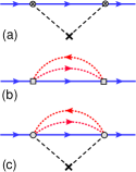
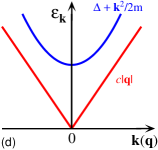
Figure 1: (Color online) (a)-(c) Diagrams representing impurity, magnon-magnon, and impurity-assisted scattering of the optical magnon (solid lines). Dotted lines are acoustic magnons. (d) Schematic energy spectrum of the model (1).

Theory.—We begin with the spin Hamiltonian of a collinear AF with an easy-plane anisotropy induced by the single-ion term $D>0$:

$${\cal H}=\sum_{\langle ij\rangle}J_{ij}\,{\bf S}_{i}\cdot{\bf S}_{j}+D\sum_{i}\left(S^{z}\right)^{2}\,.$$ (1)

Two examples are the nearest-neighbor AFs on square and honeycomb lattices. The latter model, with the non-frustrating third-neighbor exchange, is relevant to the spin-1 antiferromagnet $\rm BaNi_{2}(PO_{4})_{2}$ Regnault discussed below.

As a consequence of broken $XY$ symmetry, excitation spectrum in the ordered antiferromagnetic state possesses acoustic ($\alpha$) and gapped ($\beta$) magnon branches:

$$\varepsilon^{\alpha}_{\bf k}\approx c|{\bf k}|\ ,\qquad\varepsilon^{\beta}_{\bf k}\approx\Delta+\frac{{\bf k}^{2}}{2m}\ ,$$ (2)

see Fig. 1(d) for a sketch. Explicit expressions for $c$, $\Delta$, and $m$ for BaNi₂(PO₄)₂ are provided in suppl .

Defects are present in all crystals. While vacancies and substitutions may be eliminated in some materials, inhomogeneous lattice distortions remain an intrinsic source of disorder, inducing weak random variations $\delta J$ and $\delta D$ of microscopic parameters in the spin Hamiltonian (1) Kohama11 . Both types of randomness have qualitatively the same effect on magnon lifetimes. For example, local modification of the single-ion anisotropy $\delta D(S^{z}_{\ell})^{2}$ generates scattering potential for magnons

$${\cal H}_{2}^{\rm imp}=\sum_{\bf k,k^{\prime}}e^{i({\bf k-k^{\prime}}){\bf R}_{\ell}}\,U_{{\bf k}{\bf k^{\prime}}}\,c_{\bf k^{\prime}}^{\dagger}c_{\bf k}\ ,$$ (3)

where $c_{\bf k}\!=\!\alpha_{\bf k}(\beta_{\bf k})$, $U_{{\bf k}{\bf k^{\prime}}}\!=\!\delta DS\,(u_{\bf k}\!+\!v_{\bf k})(u_{\bf k^{\prime}}\!+\!v_{\bf k^{\prime}})$, and $u_{\bf k},v_{\bf k}$ are the Bogolyubov transformation parameters. For optical magnons at ${\bf k},{\bf k}^{\prime}\to 0$, the momentum dependence is not important, $U_{{\bf k}{\bf k^{\prime}}}\!=\!O(\delta D)$. For bond disorder, all expressions are the same with a substitution $\delta D\!\to\!\delta J$ and an additional phase factor, which depends on bond orientation and disappears after impurity averaging.

For the gapped magnons with ${\bf k}\rightarrow 0$, scattering amplitude in the second Born approximation, Fig. 1(a), averaged over spatial distribution of impurities is Mahan

$$\Gamma^{\rm imp}_{\bf k}\approx\Gamma_{0}\propto n_{i}\overline{U}^{2}_{i}\,\frac{m\,\omega_{\rm max}^{2}}{\Delta^{2}}\,,$$ (4)

where $n_{i}$ is the impurity concentration, $\overline{U}_{i}=O(\delta J,\delta D)$ is the averaged impurity potential, and $\omega_{\rm max}$ is the magnon bandwidth suppl . Thus, in 2D, conventional impurity scattering results in a finite zero-temperature relaxation rate of the gapped magnons.

At low temperatures, the principal scattering channel for optical magnons is due to collisions with the thermally excited acoustic spin waves with $cq\sim T\ll\Delta$. All other processes are either forbidden kinematically or exponentially suppressed. In this case we can consider only $\beta\alpha\rightarrow\beta\alpha$ terms in the magnon-magnon interaction:

$${\cal H}_{4}^{\rm mm}=\sum_{\bf k+q=k^{\prime}+q^{\prime}}V^{\rm mm}_{\bf kq;k^{\prime}q^{\prime}}\beta_{\bf k^{\prime}}^{\dagger}\alpha_{\bf q^{\prime}}^{\dagger}\alpha^{\phantom{{\dagger}}}_{\bf q}\beta^{\phantom{{\dagger}}}_{\bf k}\,,$$ (5)

$${\cal H}_{4}^{\rm imp}=\sum_{\bf kq,k^{\prime}q^{\prime}}e^{i\Delta{\bf k}{\bf R}_{\ell}}\,V^{\rm\,imp}_{\bf k,q;k^{\prime},q^{\prime}}\beta_{\bf k^{\prime}}^{\dagger}\alpha_{\bf q^{\prime}}^{\dagger}\alpha^{\phantom{{\dagger}}}_{\bf q}\beta^{\phantom{{\dagger}}}_{\bf k}\,,\ \ \ \$$ (6)

where the first and the second row correspond to the conventional and to the impurity-assisted magnon-magnon scattering, respectively, with $\Delta{\bf k}\!=\!{\bf k}\!+{\bf q}\!-{\bf q^{\prime}}\!-{\bf k^{\prime}}$. The latter is of the same origin as the conventional impurity scattering in (3) since $\delta D$ and $\delta J$ also modify locally interactions among magnons suppl . In the one-loop approximation, (5) and (6) yield the self-energies of Figs. 1(b) and (c). Applying standard Matsubara technique, relaxation rates can be expressed as

$$\Gamma^{{\rm mm}}_{\bf k}=\pi\sum_{\bf qq^{\prime}}\left|V^{\rm mm}_{\bf kq;k^{\prime}q^{\prime}}\right|^{2}N^{\bf q}_{{\bf k^{\prime}}{\bf q^{\prime}}}\,\delta(\Delta\varepsilon)\ ,$$ (7)

$$\Gamma^{{\rm imp},T}_{\bf k}=\pi n_{i}\sum_{\bf qq^{\prime}k^{\prime}}\left|\bar{V}^{\rm\,imp}_{\bf kq;k^{\prime}q^{\prime}}\right|^{2}N^{\bf q}_{{\bf k^{\prime}}{\bf q^{\prime}}}\,\delta(\Delta\varepsilon)\ ,$$ (8)

where $\Delta\varepsilon=\varepsilon_{\bf k}\!+\varepsilon_{\bf q}\!-\varepsilon_{\bf q^{\prime}}\!-\varepsilon_{\bf k^{\prime}}$, $N^{\bf q}_{{\bf k^{\prime}}{\bf q^{\prime}}}=n_{\bf q}(1+n_{\bf q^{\prime}}\!+n_{\bf k^{\prime}})-n_{\bf q^{\prime}}n_{\bf k^{\prime}}$, and $n_{\bf q}$ is the Bose factor.

There are two important differences between $\Gamma^{{\rm mm}}$ and $\Gamma^{{\rm imp},T}$ in (7) and (8). First, the total momentum is not conserved for impurity scattering. This relaxes kinematic constraints of the 4-magnon scattering processes, but requires instead integration over the extra independent momentum $\bf k^{\prime}$. Second and most crucial, interaction vertices $V^{\rm mm}_{\bf kq;k^{\prime}q^{\prime}}$ and $V^{\rm imp}_{\bf kq;k^{\prime}q^{\prime}}$ show very different long-wavelength behavior as ${\bf q}$, ${\bf q}^{\prime}\rightarrow 0$. We calculate them using the approach similar to HKHH ; Rezende , and find that in the long-wavelength limit magnon-magnon interaction (5) is $V^{\rm mm}_{\bf kq;k^{\prime}q^{\prime}}\propto\sqrt{qq^{\prime}}$, in accordance with the hydrodynamic limit LLIX . However, for the impurity-assisted scattering (6), interaction is $V^{\rm\,imp}_{\bf kq;k^{\prime}q^{\prime}}\propto 1/\sqrt{qq^{\prime}}$. This can be understood as a consequence of an effective long-range potential for acoustic magnons produced by the gaped magnon while in the vicinity of an impurity.

The leading $T$-dependence of $\Gamma^{{\rm mm}}_{{\bf k}\rightarrow 0}$ and $\Gamma^{{\rm\,imp},T}_{{\bf k}\rightarrow 0}$ can be calculated now using (2) and approximating interaction vertices with their long-wavelength expressions. The main contribution to the integrals in (7) and (8) is determined by acoustic magnons with $q,q^{\prime}\!\sim\!T/c$. Then, a straightforward power counting yields

$$\Gamma^{{\rm mm}}_{{\bf k}\rightarrow 0}\approx B\left(\frac{T}{\omega_{max}}\right)^{5},$$ (9)

where $B\sim\omega_{max}$ suppl . Thus, the inverse lifetime of an optical magnon is proportional to $T^{5}$ in 2D. A generalization to higher dimensions gives $\Gamma^{{\rm mm}}\propto T^{2D+1}$. The $T^{7}$-law for the relaxation rate of optical magnons in 3D AFs was previously predicted in Baryakhtar73 . We note that for a given model, the effect of magnon-magnon scattering in (9) can be calculated using microscopic parameters, thus putting strict bounds on its magnitude.

The same calculation for $\Gamma^{{\rm imp},T}_{{\bf k}\rightarrow 0}$ proceeds via the following integral:

$$\Gamma^{{\rm imp},T}_{{\bf k}\rightarrow 0}\approx\frac{n_{i}\overline{U}_{i}^{2}}{8\pi^{2}}\int_{q}\int_{q^{\prime}}n_{\bf q}\left(n_{{\bf q}^{\prime}}+1\right)\int_{0}^{\infty}k^{\prime}\,dk^{\prime}\,\delta\left(\Delta\varepsilon\right),\$$ (10)

where $\int_{q}\!=\!\int_{0}^{\Lambda}dq$ with $\Lambda\!\sim\!\pi/a$, $\Delta\varepsilon\!=\!cq\!-\!cq^{\prime}\!-\!k^{\prime 2}/2m$, and we used the relation between $\bar{V}^{\rm\,imp}_{\bf kq;k^{\prime}q^{\prime}}$ in (6) and $U_{{\bf k}{\bf k^{\prime}}}$ in (3). The naïve power counting in (10) already gives $\Gamma^{{\rm imp},T}\!\propto\!T^{2}$, while a more careful consideration shows further enhancement of the scattering as the integrals formally diverge [logarithmically] in the ${q}\rightarrow 0$ region, demonstrating an important role of the long-wavelength magnons in 2D. This divergence is similar to the one in the problem of finite $T_{N}$ ordering temperature in 2D and is regularized similarly by introducing low-energy cutoff. The cutoff is either due to a 3D-crossover as in the case of some cuprates cuprates , or a weak in-plane anisotropy that induces small gap $\omega_{0}$ in the acoustic branch, the case directly relevant to the current work Regnault ; Ikeda .

Combining (4) and (10) we obtain impurity-induced relaxation rate of gapped magnons

$$\Gamma^{{\rm imp}}\approx\Gamma_{0}+A\biggl{(}\frac{T}{\omega_{max}}\biggr{)}^{2}\left[\biggl{(}\ln{\frac{T}{\omega_{0}}}\biggr{)}^{2}+\frac{\pi^{2}}{3}\right]\,,$$ (11)

where both $\Gamma_{0}$ and $A$ are proportional to $n_{i}$ and to the average strength of disorder $\overline{U}_{i}^{2}$. As a result, the impurity scattering leads to a relaxation rate that carries a significantly lower power of temperature than the magnon-magnon scattering mechanism. Therefore, despite possible smallness of the combined impurity concentration and strength, it should dominate not only the $T=0$ lifetime of the gapped magnon, but also its temperature dependence in the entire low-temperature regime. A qualitative prediction of our consideration is that $\Gamma_{0}$ and $A$ in (10) should be of the same order since both terms are related to disorder. In addition, for samples of the same material of different quality, they must scale with the amount of structural disorder in a correlated way.

In the 3D case, impurity-assisted mechanism (10) gives $\Gamma^{{\rm imp},T}_{3D}\propto T^{9/2}$, still dominating the 3D magnon-magnon relaxation rate $\Gamma^{{\rm mm}}_{3D}\propto T^{7}$ discussed above.

Experiment.—The experimental part of our work is devoted to the neutron spin-echo measurements of the magnon lifetime in $\rm BaNi_{2}(PO_{4})_{2}$. This material is a layered quasi-2D AF with a honeycomb lattice of spin-1 Ni²⁺ ions and Néel temperature $T_{N}\!\approx\!25$ K. A comprehensive review of the physical properties of $\rm BaNi_{2}(PO_{4})_{2}$ is presented in Regnault . Its excitation spectrum has an optical branch with the gap $\Delta\approx 32$ K and an acoustic mode, as is sketched in Fig. 1(d). The fit of the magnon dispersion yields the following microscopic parameters: $J_{1}\!=\!0.38$ meV and $J_{3}\!=\!1.52$ meV are exchanges between first- and third-neighbor spins, and $D\!=\!0.32$ meV is the single-ion anisotropy. The thermodynamic properties of BaNi₂(PO₄)₂ follow the 2D behavior down to $T\!\lesssim\!1$K and a small gap in the acoustic branch, $\omega_{0}\!\approx\!2$K, due to weak in-plane anisotropy is consistent with the value of the ordering temperature Regnault .

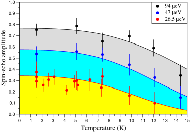
Figure 2: (Color online) Temperature dependence of the polarization (spin-echo amplitude) of the neutron beam $P(T)$ for several representative spin-echo energies.

The spin-echo experiments were performed on the triple-axis spectrometer IN22 (ILL, Grenoble) by using ZETA neutron resonance spin-echo option Martin11 . The incident neutron beam was polarized and the scattered beam analyzed from (111) reflection of $\rm Cu_{2}MnAl$ Heusler alloy focusing devices. We used a fixed-$k_{f}$ configuration, with $k_{f}=2.662$ Å^-1 or $k_{f}=1.97$ Å^-1. Different rf-flipper configurations were used in order to adapt the spin-echo time (energy) $t_{\rm NSE}$ ($\varepsilon_{\rm NSE}=h/t_{\rm NSE}$) to the magnetic excitation lifetimes, typically in the range of $5-50\,$ps ($130-13\,\mu$eV). As for any spin-echo experiment Mezei72 ; Golub87 , the measurement of the neutron polarization (spin-echo amplitude) after the scattering, $P(t_{\rm NSE})$, provides us with a direct access to the correlation function $S({\bf q},t_{\rm NSE})$. For a spin-wave excitation described by a Lorentzian function in energy of half width $\Gamma$, one can show that $P(\varepsilon_{\rm NSE})\!=\!P_{0}(\varepsilon_{\rm NSE})\exp({-\Gamma/\varepsilon_{\rm NSE}})$, in which the prefactor $P_{0}$ depends on the spin-echo resolution.

For our measurements, we have used a $2\;\textrm{cm}^{3}$ single crystal of $\rm BaNi_{2}(PO_{4})_{2}$ oriented with the ${\bf a}^{*}$ and ${\bf c}^{*}$ reciprocal axes in the scattering plane. The spin-echo data were taken at the antiferromagnetic scattering vector ${\bf Q}_{\rm AF}=(1,0,0)$ and the energy transfer $\Delta E=3$ meV corresponding to the bottom of the dispersion curve of the gapped mode Regnault . In determining the spin-echo amplitudes, neutron intensities were corrected for the inelastic background, measured at the scattering vector ${\bf Q}_{\rm AF}$ and the energy transfer $\Delta E=5$ meV. Results of the temperature dependence of spin-echo amplitudes for several representative $\varepsilon_{\rm NSE}$’s are shown in Fig. 2. Solid lines are the fits of the spin-echo amplitudes with $P\!=\!P_{0}e^{-\Gamma/\varepsilon_{NSE}}$ using relaxation rate in the functional form given by (9) and (11), $\Gamma\!=\!\Gamma^{\rm mm}+\Gamma^{\rm imp}$, which we discuss next. Using the full set of $P(T,\varepsilon_{\rm NSE})$ data, experimental results for $\Gamma(T)$ are extracted from the fits of $\ln(P)$ vs $\varepsilon_{\rm NSE}$ at fixed temperatures. These results are presented in our Fig. 3 together with the theoretical fits.

Comparison.—The relaxation rate approaches the constant value of $\Gamma_{0}\!\approx\!25$ $\mu$eV at $T\!\rightarrow\!0$, in agreement with the expectation (4) for the gapped mode in 2D. The low-$T$ dependence of the relaxation rate is following the power law much slower than $T^{5}$. The quality of the free-parameter fit of $\Delta\Gamma\!=\!\Gamma(T)\!-\!\Gamma_{0}$ with just the $T^{5}$ law is not satisfactory for either $\Gamma(T)$ or $P(T)$’s in Figs. 3 and 2, and the magnitude of $\Delta\Gamma$ also requires an unphysically large values of the magnon-magnon scattering parameter $B$ in (9), exceeding theoretical estimates roughly tenfold. On the other hand, $T^{2}\ln^{2}T$ law gives much more satisfactory fits in the low- and intermediate-$T$ regime up to 12 K in both $\Gamma(T)$ and $P(T)$, shown as a separate fit by the dotted line in Fig. 3. The best fit of $\Gamma(T)$, given by solid line, is the sum of the magnon-magnon and impurity-scattering effects from (9) and (11), with the magnon-magnon and impurity-assisted parameters $B\!=\!15$ meV and $A\!=\!90$ $\mu$eV, respectively. The same $\Gamma(T)$ is used in all three curves of $P(T)$ in Fig. 2, the original data from which experimental $\Gamma(T)$ is extracted. Magnon bandwidth $\omega_{max}\!=\!64$ K and the low-energy cutoff $\omega_{0}\!=\!2$ K, equal to the gap in the acoustic branch, were used.

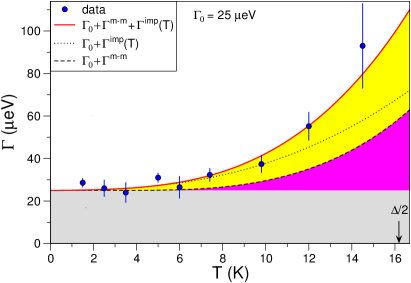
Figure 3: (Color online) Temperature dependence of the relaxation rate $\Gamma$ of the optical magnon with ${\bf k}\approx 0$ in BaNi₂(PO₄)₂. Full line is the best theoretical fit including all contributions with parameters described in the text. Dashed and dotted lines indicate separate contributions of magnon-magnon and impurity-assisted magnon-magnon scattering.

Two remarks are in order concerning the role of the magnon-magnon relaxation rate used in Fig. 3. First, fits of $\Gamma(T)$ in Fig. 3 also include a contribution from scattering off the thermally excited optical magnons, which is given by $\Gamma^{\rm rr}\!=\!C\left(\frac{T}{\Delta}\right)e^{-\Delta/T}$ suppl . Its contribution is roughly equal to that of the $T^{5}$-term (9) at $T\!=\!16$K ($=\!\Delta/2$), but diminishes faster at lower $T$. In the fit of $\Gamma(T)$ we use the value of $C\!=\!260$ $\mu$eV, about three times the theory estimate: $C^{th}\!\approx\!70$ $\mu$eV. Second, the theoretical estimate of the magnon-magnon interaction parameter in $T^{5}$ law (9) is $B^{th}\!\approx\!6$ meV, again factor 2.5 smaller than the one used in the fit ($B\!=\!15$ meV). Altogether, the magnon-magnon contribution to $\Gamma(T)$, shown by the dashed line and the corresponding color shading in Fig. 3, is likely a generous overestimate of its actual role in the relaxation.

Still, the contribution of the impurity-assisted mechanism in $\Gamma(T)$ is very strongly pronounced and is not explicable by the conventional scattering mechanisms. For example, at 12K the impurity scattering accounts for at least 2/3 of the temperature-dependent part of $\Gamma(T)$. The parameter of the impurity-assisted term in (11) used in the fit is $A\!=\!90\mu$eV, which is of the same order with the constant impurity term $\Gamma_{0}$, meeting our expectations outlined above. This is, again, the strong argument that both the constant and the $T$-dependent terms in the relaxation rate must have the same origin, giving further support to the consistency of our explanation of the data.

The values of $A$ and $\Gamma_{0}$ cannot be determined theoretically as the impurity concentration and strength are, generally, unknown. However, another consistency check is possible: the ratio of $\Gamma_{0}$ to a characteristic energy scale of the problem, $\omega_{max}$, should give, according to (4), an estimate of the cumulative measure of disorder concentration and its strength: $n_{\rm imp}(\overline{\delta D}/D)^{2}\!\approx\!\Gamma_{0}/\omega_{max}\!\approx\!5\cdot 10^{-3}$. This translates into a reasonable estimate of the disorder and its strength in BaNi₂(PO₄)₂: modulation of magnetic couplings is equivalent to half of a percent of sites having $\delta D$ ($\delta J$) of order $D$ ($J$). The amount of structural distortion in BaNi₂(PO₄)₂ Larmor12 is consistent with the magnitude of such variations of magnetic couplings, given the strong spin-lattice coupling in this material.

Other systems.—We propose that similar, and even stronger, effects of disorder in the relaxation rate must be present in the 2D noncollinear AFs, in which magnon-magnon interactions acquire the so-called cubic interaction terms ZhCh , absent in the collinear AFs considered above. The self-energies associated with such interaction are the same as in Figs. 1(b) and (c), but with two intermediate lines instead of three. With the long-wavelength behavior of the impurity interaction to follow $\delta V_{3}({\bf k},{\bf q})\!\propto\!1/\sqrt{q}$, as in the considered case, a qualitative consideration similar to (10) leads to:

$$\Gamma^{{\rm imp},T}_{{\bf k}\rightarrow 0}\approx A_{3}\,\left(\frac{T}{\omega_{max}}\right)\,\ln{\frac{T}{\omega_{0}}}\,,$$ (12)

where $A_{3}\!\propto\!n_{\rm imp}(\overline{\delta D}/D)^{2}$, an even lower power of $T$. Since the canting of spins can be induced by the external field, we propose an experimental investigation of the effect of such a field on the relaxation rate. For the 3D noncollinear AFs we predict $\Gamma^{{\rm imp},T}\propto T^{5/2}$.

Recent neutron spin-echo experiment in a Heisenberg-like AF MnF₂ Bayrakci06 have reported significant discrepancies between measured relaxation rates and predictions of the magnon-magnon scattering theory HKHH ; Rezende , precisely in the regime of low-$T$ and small-${\bf k}$ where the theory is assumed to be most reliable. Although the current work concerns the dynamics of strongly gapped excitations and our results are not directly transferable to the case of MnF₂, we have, nevertheless, presented a general case in which the magnon-magnon scattering mechanism is completely overshadowed by impurity scattering, thus suggesting a similar consideration in other systems.

Conclusions.—To conclude, we have presented strong evidence of the general situation in which temperature-dependence of the relaxation rate of a magnetic excitation is completely dominated by the effects induced by simple structural disorder. Our results are strongly supported by the available experimental data. Further theoretical and experimental studies are suggested.

This work was initiated at the Max-Planck Institute for the Physics of Complex Systems during the activities of the Advanced Study Group Program on “Unconventional Magnetism in High Fields,” which we would like to thank for hospitality. The work of A. L. C. was supported by the DOE under Grant No. DE-FG02-04ER46174.

Spin Hamiltonian

Here we briefly outline basic steps and main results of the spin-wave calculations for the energy spectrum and the magnon relaxation rates of the $J_{1}$–$J_{3}$ antiferromagnet on a honeycomb lattice. The harmonic spin-wave analysis of the nearest-neighbor Heisenberg honeycomb-lattice antiferromagnet can be found, for example, in Weihong91sup .

Geometry of exchange bonds of the considered model is schematically shown in Fig. 4. The unit cell of the antiferromagnetic structure coincides with the crystal unit cell and contains two oppositely aligned spins ${\bf S}_{1,i}$ and ${\bf S}_{2,i}$ in positions $(0,0)$ and $\bm{\rho}=(a/\sqrt{3},0)$. The elementary translation vectors are defined as ${\bf a}_{1}=a(\sqrt{3}/2,-1/2)$ and ${\bf a}_{2}=a(0,1)$. The lattice constant in BaNi₂(PO₄)₂ is equal to $a=4.81$ Å. The reciprocal lattice basis is ${\bf b}_{1}=4\pi/(\sqrt{3}a)(1,0)$ and ${\bf b}_{2}=2\pi/(\sqrt{3}a)(1,\sqrt{3})$. The volume of the Brilouin zone is $V_{\rm BZ}=8\pi^{2}/\sqrt{3}a^{2}$.

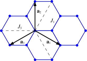
Figure 4: $J_{1}$–$J_{3}$ model in a honeycomb lattice.

The spin Hamiltonian includes Heisenberg exchange interactions between first- and third-neighbor spins together with the single-ion anisotropy:

$$\hat{\cal H} = J_{1}\sum_{i}{\bf S}_{1,i}\cdot({\bf S}_{2,i}+{\bf S}_{2,i-1}+{\bf S}_{2,i+3})$$

$$+ J_{3}\sum_{i}{\bf S}_{1,i}\cdot({\bf S}_{2,i+2}+{\bf S}_{2,i-2}+{\bf S}_{2,i-1+3})$$

$$+ D\sum_{i}\bigl{[}(S_{1,i}^{z})^{2}+(S_{2,i}^{z})^{2}\bigr{]}\ .$$

Here ${\bf S}_{2,i-1}$ denotes spin in the unit cell ${\bf R}_{i}-{\bf a}_{1}$ and so on. The microscopic parameters for BaNi₂(PO₄)₂ ($S=1$) were determined from the magnon dispersion as $J_{1}=0.38$ meV, $J_{3}=1.52$ meV, and $D=0.34$ meV Regnaultsup . The second-neighbor exchange was estimated to be much smaller $J_{2}=0.05$ meV and is neglected in the following.

Applying the Holstein-Primakoff transformation for two antiferromagnetic sublattices and performing the Fourier transformation

$$a_{i}=\frac{1}{N^{1/2}}\sum_{\bf k}e^{i{\bf k}{\bf R}_{i}}a_{\bf k}\,,\quad b_{i}=\frac{1}{N^{1/2}}\sum_{\bf k}e^{i{\bf k}({\bf R}_{i}+\bm{\rho})}b_{\bf k}\,,$$ (14)

we obtain the harmonic part of the boson Hamiltonian

$$\hat{\cal H}_{2} = S\sum_{\bf k}\Bigl{[}(3J_{13}+D)(a^{\dagger}_{\bf k}a_{\bf k}+b^{\dagger}_{\bf k}b_{\bf k})$$

$$- a_{\bf k}b_{-\bf k}F^{*}_{\bf k}+\frac{D}{2}\,(a_{\bf k}a_{-\bf k}+b_{\bf k}b_{-\bf k})+\textrm{h.\,c.}\Bigr{]}\ ,$$

where we use the shorthand notations

$$J_{13}=J_{1}+J_{3}\,,$$ (16)

$$F_{\bf k}=J_{1}\bigl{(}e^{i{\bf k}_{1}}+e^{i{\bf k}_{2}}+e^{i{\bf k}_{3}}\bigr{)}+J_{3}\bigl{(}e^{i{\bf k}_{4}}+e^{i{\bf k}_{5}}+e^{i{\bf k}_{6}}\bigr{)},$$

with ${\bf k}_{n}={\bf k}\cdot{\bf r}_{n}$ and

$${\bf r}_{1}=\frac{a}{\sqrt{3}}(1,0)\,,\quad{\bf r}_{2,3}=\frac{a}{\sqrt{3}}\Bigl{(}-\frac{1}{2},\pm\frac{\sqrt{3}}{2}\Bigr{)}\,,$$

$${\bf r}_{4,5}=\frac{a}{\sqrt{3}}(1,\pm\sqrt{3})\ ,\quad{\bf r}_{6}=\frac{a}{\sqrt{3}}(-2,0)\ .$$ (17)

Diagonalization of the quadratic form (Spin Hamiltonian) with the help of the canonical Bogolyubov transformation yields

$$\hat{\cal H}_{2}=\sum_{\bf k}\Bigl{[}\varepsilon_{\alpha}({\bf k})\alpha^{\dagger}_{\bf k}\alpha_{\bf k}+\varepsilon_{\beta}({\bf k})\beta^{\dagger}_{\bf k}\beta_{\bf k}\Bigr{]}\ ,$$ (18)

where excitation energies are

$$\varepsilon_{\alpha}({\bf k})=S\sqrt{(3J_{13}-|F_{\bf k}|)(3J_{13}+|F_{\bf k}|+2D)}\ ,$$ (19)

$$\varepsilon_{\beta}({\bf k})=S\sqrt{(3J_{13}+|F_{\bf k}|)(3J_{13}-|F_{\bf k}|+2D)}\ .$$ (20)

The first magnon branch is gapless, $\varepsilon_{\alpha}(0)=0$, and reaches the maximum value of

$$\omega^{\alpha}_{\rm max}=S\sqrt{(2J_{3}\!+4J_{1})(4J_{3}\!+2J_{1}+2D)}\approx 5.9\ \textrm{meV}$$ (21)

at ${\bf k}=[q,q]$ with $q\approx 0.25$ in the reciprocal lattice units. The second branch describes optical magnons with a finite energy gap at ${\bf k}=0$

$$\Delta=2S\sqrt{3DJ_{13}}\approx 2.8\ \textrm{meV}\ .$$ (22)

The maximum of the optical branch $\omega^{\beta}_{\rm max}$ is close to (21).

Long-wavelength limit

In the long-wavelength limit $k\to 0$ the energy of the acoustic branch has linear dispersion $\varepsilon_{\alpha}({\bf k})\approx c(ka)$ with the spin-wave velocity

$$c=S\sqrt{2(J_{3}+{\textstyle\frac{1}{4}}J_{1})(3J_{13}+D)}=4.42\ \textrm{meV}\ .$$ (23)

For the optical branch one finds

$$\varepsilon_{\beta}({\bf k})\approx\Delta+\frac{(ka)^{2}}{2m}\,,\ \ m=\frac{(3DJ_{13})^{1/2}}{S(J_{3}\!+{\textstyle\frac{1}{4}}J_{1})(3J_{13}\!-D)}\,,$$ (24)

with $m=0.16$ meV^-1 for BaNi₂(PO₄)₂.

For small $k$ the Bogolyubov transformation can be written explicitly in the following way. First, we transform from the original Holstein-Primakoff bosons $a_{i}$ and $b_{i}$ to their linear combinations:

$$\bar{a}_{i}=\frac{1}{\sqrt{2}}(a_{i}-b_{i})\ ,\quad\bar{b}_{i}=\frac{1}{\sqrt{2}}(a_{i}+b_{i})\ .$$ (25)

The Fourier transformed Hamiltonian (Spin Hamiltonian) takes the following form

$$\hat{\cal H}_{2} = S\sum_{\bf k}\Bigl{[}(3J_{13}+D)(\bar{a}^{\dagger}_{\bf k}\bar{a}_{\bf k}+\bar{b}^{\dagger}_{\bf k}\bar{b}_{\bf k})$$

$$+ \frac{1}{2}(D+|F_{\bf k}|)\,\bar{a}_{\bf k}\bar{a}_{-\bf k}\!+\frac{1}{2}(D-|F_{\bf k}|)\,\bar{b}_{\bf k}\bar{b}_{-\bf k}\!+\textrm{h.\,c.}\Bigr{]}\,.$$

Second, the standard $u$–$v$ transformation is applied separately for $\bar{a}_{\bf k}$ and $\bar{b}_{\bf k}$ bosons. In particular, for the acoustic branch, $\bar{a}_{\bf k}=u_{k}\alpha_{\bf k}+v_{k}\alpha^{\dagger}_{-\bf k}$, we obtain

$$u_{k} \approx \sqrt{\frac{1+d}{2\tilde{c}ka}}\Bigl{(}1+\frac{\tilde{c}ka}{2(1+d)}\Bigr{)}\ ,$$

$$v_{k} \approx -\sqrt{\frac{1+d}{2\tilde{c}ka}}\Bigl{(}1-\frac{\tilde{c}ka}{2(1+d)}\Bigr{)}\ ,$$ (27)

where $d=D/(3J_{13})$ and $\tilde{c}=c/(3J_{13})$. In the case of BaNi₂(PO₄)₂ the two dimensionless constants are $d\approx 0.06$ and $\tilde{c}\approx 0.77$.

Similarly, for optical magnons with $k\to 0$ we obtain $\bar{b}_{\bf k}=u_{\bf k}\beta_{\bf k}+v_{\bf k}\beta^{\dagger}_{-\bf k}$ with

$$u_{0}^{2}+v_{0}^{2}=\frac{1+d}{2\sqrt{d}}\ ,\quad 2u_{0}v_{0}=\frac{1-d}{2\sqrt{d}}\ .$$ (28)

Magnon-magnon interaction

For a collinear antiferromagnet the interaction between spin-waves is described by four-magnon terms in the bosonic Hamiltonian. The four-magnon terms of the exchange origin are expressed as

$$H^{\rm(ex)}_{4} = -\frac{1}{N}\sum_{1+2=3+4}F_{{\bf k}_{3}-{\bf k}_{2}}a_{4}^{\dagger}b_{3}^{\dagger}b_{2}a_{1}$$

$$+ \frac{1}{4N}\sum_{1+2+3=4}F_{{\bf k}_{1}}\Bigl{(}a_{4}^{\dagger}a_{3}a_{2}b_{1}+b_{4}^{\dagger}b_{3}b_{2}a_{1}+\textrm{h.\,c.}\Bigr{)},$$

where $a_{1}$ stands for $a_{{\bf k}_{1}}$ etc. The single-ion anisotropy contributes

$$H^{\rm(an)}_{4} = -\frac{D}{2N}\sum_{1+2=3+4}\bigl{(}a_{4}^{\dagger}a_{3}^{\dagger}a_{2}a_{1}+b_{4}^{\dagger}b_{3}^{\dagger}b_{2}b_{1}\bigr{)}$$

$$- \frac{D}{4N}\sum_{1+2+3=4}\bigl{(}a_{4}^{\dagger}a_{3}a_{2}a_{1}+b_{4}^{\dagger}b_{3}b_{2}b_{1}+\textrm{h.\,c.}\bigr{)}.$$

Performing transformation from $a_{\bf k}$, $b_{\bf k}$ to $\alpha_{\bf k}$, $\beta_{\bf k}$ we obtain various magnon-magnon terms. The scattering of optical ($\beta$) magnons on each other, which will be referred to as the roton-roton interaction, can be straightforwardly written as

$$V^{\rm rr} = -\frac{3J_{13}+D}{N}\sum_{1+2=3+4}\beta_{4}^{\dagger}\beta_{3}^{\dagger}\beta_{2}\beta_{1}\ .$$ (31)

Derivation of the roton-phonon interaction (scattering of the optical magnon on the acoustic one, $\beta$ on $\alpha$) is more involved and we obtain an estimate as

$$V^{\rm rp}=-\frac{3(J_{3}+\frac{1}{4}J_{1})(1+d)^{2}}{4\sqrt{3d}\,\tilde{c}N}\!\!\!\sum_{1+2=3+4}\!\!\!\sqrt{k_{2}k_{3}}\,\beta_{4}^{\dagger}\alpha_{3}^{\dagger}\alpha_{2}\beta_{1}\ .$$ (32)

The individual terms in the magnon-magnon interaction obtained from (Magnon-magnon interaction) and (Magnon-magnon interaction) applying the Bogolyubov transformation are proportional to $u_{\bf q}u_{\bf q^{\prime}}$ and diverge for scattering processes involving acoustic magnons, see (27). However, the leading $\sim{\cal O}(1/\sqrt{qq^{\prime}})$ and the subleading singularity $\sim{\cal O}(1)$ cancel out in their net contribution and $V^{\rm rp}_{\bf kq;k^{\prime}q^{\prime}}\propto\sqrt{qq^{\prime}}$ in agreement with the hydrodynamic approach Baryakhtar73sup ; LLIXsup .

Local modulation of magnetic coupling constants due to structural disorder, etc., will result in independent variations of $J$- and $D$-terms in magnon-magnon interaction in (Magnon-magnon interaction) and (Magnon-magnon interaction). Thus, the resultant impurity-assisted magnon-magnon interaction will retain the same structure as the magnon-magnon interaction, with two important differences. First, the momentum in such a scattering is not conserved, and, second, the variation of $J$ ($\delta J$) is associated only with (Magnon-magnon interaction) and the variation $\delta D$ will contain only (Magnon-magnon interaction) part. Since such variations are independent, it suffices to consider one of them and treat the associated constant as a free parameter. The most important consequence of this consideration is that, in the impurity scattering, there is no cancellation of the individual terms that are proportional to $u_{\bf q}u_{\bf q^{\prime}}\propto 1/\sqrt{qq^{\prime}}$, compared to the case of magnon-magnon scattering in (32) discussed above where such a cancellation does take place. Thus, in the long-wavelength limit, $V^{\rm\,imp}_{\bf kq;k^{\prime}q^{\prime}}\propto 1/\sqrt{qq^{\prime}}$, with a coefficient proportional to the impurity concentration and strength of the disorder.

Relaxation rate of optical magnons

The lowest-order diagram for the magnon self-energy calculated using Matsubara technique is

$$\Sigma({\bf k},i\omega) = \frac{1}{2}\sum_{{\bf q},{\bf q}^{\prime}}\frac{\big{|}V_{\bf k}({\bf q},{\bf q}^{\prime})\big{|}^{2}}{i\omega+\varepsilon_{\bf q}\!-\varepsilon_{\bf q^{\prime}}\!-\varepsilon_{\bf k^{\prime}}}$$

$$\times [n_{\bf q}(n_{\bf q^{\prime}}\!+1)(n_{\bf k^{\prime}}+1)-(n_{\bf q}\!+1)n_{\bf q^{\prime}}n_{\bf k^{\prime}}]$$

with $\bf k^{\prime}=k+q-q^{\prime}$. Then the damping rate is

$$\Gamma_{\bf k} = \frac{\pi}{2}\,\sum_{{\bf q},{\bf q}^{\prime}}\big{|}V_{\bf k}({\bf q},{\bf q}^{\prime})\big{|}^{2}[n_{\bf q}(1\!+n_{\bf q^{\prime}}\!+n_{\bf k^{\prime}})-n_{\bf q^{\prime}}n_{\bf k^{\prime}}]$$ (34)

$$\times \delta(\varepsilon_{\bf k}+\varepsilon_{\bf q}-\varepsilon_{\bf q^{\prime}}-\varepsilon_{\bf k^{\prime}})\,.$$

First, we consider the roton-roton scattering processes. The low-temperature asymptote of (34) in this case is obtained by taking $T\ll\Delta$ and keeping the leading exponentially small occupation factor. Then, for an optical magnon with ${\bf k}=0$ in two dimensions

$$\Gamma_{0}^{\rm rr} = \frac{3V_{\rm rr}^{2}}{64\pi^{2}}\int_{0}^{\infty}q\,dq\int_{0}^{q}q^{\prime}\,dq^{\prime}\int_{0}^{2\pi}d\varphi\;n_{\bf q}$$

$$\times\ \delta\left(\frac{q^{2}}{2m}-\frac{q^{\prime 2}}{2m}-\frac{|{\bf q}-{\bf q^{\prime}}|^{2}}{2m}\right).$$

Performing integration in (Relaxation rate of optical magnons) and using parameters for BaNi₂(PO₄)₂ discussed above we obtain

$$\Gamma_{0}^{\rm rr}=\frac{3(mV_{\rm rr})^{2}T}{64\pi}\,e^{-\Delta/T}\approx 0.035\,\frac{T}{\Delta}\,e^{-\Delta/T}\textrm{[meV]}\ .$$ (36)

Without going into details, there exist another channel of scattering that corresponds to a conversion of two rotons into two high-energy phonons, $\beta\beta\rightarrow\alpha\alpha$, which leads to the decay rate of the optical mode of the same exponential form as in (36) with a numerical coefficient of the same order.

Finally, the the low-temperature asymptote of the roton-phonon scattering in (34) is

$$\Gamma_{0}^{\rm rp} = \frac{3\tilde{V}_{\rm rp}^{2}}{32\pi^{2}}\int_{0}^{\infty}\!q^{2}\,dq\int_{0}^{q}q^{\prime 2}\,dq^{\prime}\int_{0}^{2\pi}\!d\varphi\>n_{\bf q}(n_{\bf q^{\prime}}\!+1)$$ (37)

$$\times \delta\left(cq-cq^{\prime}-\frac{|{\bf q}-{\bf q^{\prime}}|^{2}}{2m}\right),$$

where $V_{\rm rp}=\tilde{V}_{\rm rp}\sqrt{qq^{\prime}}$. Subsequent integration yields

$$\Gamma_{0}^{\rm rp}=\frac{\pi^{3}}{20}\frac{\tilde{V}_{\rm rp}^{2}T^{5}}{c^{6}}\approx 0.18\,\biggl{(}\frac{T}{\Delta}\biggr{)}^{5}\textrm{[meV]}\ .$$ (38)

References

- (1) S. P. Bayrakci, T. Keller, K. Habicht, and B. Keimer, Science 312, 1926 (2006).
- (2) T. Keller, P. Aynajian, K. Habicht, L. Boeri, S. K. Bose, and B. Keimer, Phys. Rev. Lett. 96, 225501 (2006).
- (3) D. Haug, V. Hinkov, P. Bourges, N. B. Christensen, A. Ivanov, T. Keller, C. T. Lin, and B. Keimer, New J. Phys. 12, 105006 (2010).
- (4) B. Náfrádi, T. Keller, H. Manaka, A. Zheludev, and B. Keimer, Phys. Rev. Lett. 106, 177202 (2011).
- (5) A. B. Harris, D. Kumar, B. I. Halperin, and P. C. Hohenberg, Phys. Rev. B 3, 961 (1971).
- (6) S. M. Rezende and R. M. White, Phys. Rev. B 14, 2939 (1976), ibid. 18, 2346 (1978).
- (7) J. Bass, W. P. Pratt, and P. A. Schroeder, Rev. Mod. Phys. 62, 645 (1990); P. L. Taylor, Phys. Rev. 135, A1333 (1964); S. Koshino, Prog. Theor. Phys. 30, 415 (1963).
- (8) R. M. White, R. Freedman, and R. B. Woolsey, Phys. Rev. B 10, 1039 (1974).
- (9) L. P. Regnault and J. Rossat-Mignod, in Magnetic Properties of Layered Transition Metal Compounds, edited by L. J. de Jongh (Kluwer Academic, Dordrecht, 1990), p. 271.
- (10) See Supplemental Material at http://link.aps.org/supplemental for details of theoretical calcualtion in the honeycomb-lattice antiferromagnets.
- (11) Y. Kohama, A. V. Sologubenko, N. R. Dilley, V. S. Zapf, M. Jaime, J. A. Mydosh, A. Paduan-Filho, K. A. Al-Hassanieh, P. Sengupta, S. Gangadharaiah, A. L. Chernyshev, and C. D. Batista, Phys. Rev. Lett. 106, 037203 (2011).
- (12) G. D. Mahan, Many-Particle Physics (Plenum Press, New York, 1990).
- (13) K. Hirakawa and H. Ikeda, in Magnetic Properties of Layered Transition Metal Compounds, edited by L. J. de Jongh (Kluwer Academic, Dordrecht, 1990), p. 231.
- (14) E. M. Lifshitz and L. P. Pitaevskii, Statistical Physics II (Pergamon, Oxford, 1980), p. 133.
- (15) M.A. Kastner, R.J. Birgeneau, G. Shirane, and Y. Endoh, Rev. Mod. Phys. 70, 897 (1998); D. C. Johnston, in Handbook of Magnetic Materials, edited by K. H. J. Buschow (Elsevier Science, North Holland, 1997).
- (16) V. G. Bar’yakhtar and V. L. Sobolev, Fiz. Tverd. Tela (Leningrad) 15, 2651 (1973) [Sov. Phys. Solid State 15, 1764 (1974)].
- (17) N. Martin, L.-P. Regnault, S. Klimko, J. E. Lorenzo, and R. Gähler, Physica B 406, 2333 (2011).
- (18) F. Mezei, Z. Physik 255, 146 (1972).
- (19) R. Golub and R. Gähler, Phys. Lett. A 123, 43 (1987).
- (20) N. Martin, L.-P. Regnault, and S. Klimko, J. Phys.: Conf. Ser. 340, 012012 (2012).
- (21) A. L. Chernyshev and M. E. Zhitomirsky, Phys. Rev. Lett. 97, 207202 (2006).

References

- (1) Z. Weihong, J. Oitmaa, and C. J. Hamer, Phys. Rev. B 44, 11869 (1991).
- (2) L. P. Regnault and J. Rossat-Mignod, in Magnetic Properties of Layered Transition Metal Compounds, edited by L. J. de Jongh (Kluwer Academic, Dordrecht, 1990), p. 271.
- (3) V. G. Bar’yakhtar and V. L. Sobolev, Fiz. Tverd. Tela 15, 2651 (1973) [Sov. Phys. Solid State 15, 1764 (1974)].
- (4) E. M. Lifshitz and L. P. Pitaevskii, Statistical Physics II (Pergamon, Oxford, 1980), p. 133.