A model of competition among more than two languages

Abstract

We extend the Abrams–Strogatz model for competition between two languages [Nature 424, 900 (2003)] to the case of $n(\geq 2)$ competing states (i.e., languages). Although the Abrams–Strogatz model for $n=2$ can be interpreted as modeling either majority preference or minority aversion, the two mechanisms are distinct when $n\geq 3$. We find that the condition for the coexistence of different states is independent of $n$ under the pure majority preference, whereas it depends on $n$ under the pure minority aversion. We also show that the stable coexistence equilibrium and stable monopoly equilibria can be multistable under the minority aversion and not under the majority preference. Furthermore, we obtain the phase diagram of the model when the effects of the majority preference and minority aversion are mixed, under the condition that different states have the same attractiveness. We show that the multistability is a generic property of the model facilitated by large $n$.

1 Introduction

The consensus problem, in which we ask whether the unanimity of one among different competing states (e.g., opinions) is reached, and its mechanisms are of interest in various disciplines including political science, sociology, and statistical physics. In models of consensus formation, it is usually assumed that each individual possesses one of the different states that can flip over time. The flip rate depends on the environment such as the number of the individuals that adopt a different state. Statistical physicists have approached this problem by analyzing a variety of models including the voter model, majority rule models, the bounded confidence model, Axelrod’s model, and the naming game (see sociophys for a review).

A major mechanism that would lead to consensus in a population is preference for the majority. Collective opinion formation under various majority voting rules has been examined for mean-field populations Chen1 ; Galam1986 ; Galam1999 ; Galam2002 ; Krapivsky ; Lambiotte4 ; Mobilia and in different types of networks such as regular lattices Chen2 ; Chen1 ; deOliveira ; Liggett ; Tessone , small-world networks PPLi , heterogeneous networks Lambiotte3 , and networks with community structure Lambiotte1 ; Lambiotte2 . The majority preference may be identified with the aversion to the minority. When there are only two states, they are equivalent because one state is the majority if and only if the other state is the minority. However, the two principles may be distinct when more than two states are assumed Volovik2009EPL . We are concerned with this case in the present study.

Language competition is an example of consensus problems. The model proposed by Abrams and Strogatz (AS model) accounts for extinction of endangered languages Abrams1 . The AS model implements competition between two languages for speakers in a population. The dynamics of the model is based on the majority preference, which is also regarded as the minority aversion because there are just two competing languages.

Several authors found that different languages can stably coexist in variants of the AS model. Two languages can coexist by spatial segregation in a model in which competition dynamics and spatial diffusion are combined Patriarca1 ; Patriarca2 . A Lotka–Volterra variant of the AS model also leads to coexistence Pinasco . Introduction of bilingual individuals also enables coexistence Mira1 ; Mira2 . Castelló and colleagues investigated variants of the AS model with bilingualism on various networks Castello1 ; Castello2 ; Castello3 ; Castello4 . Coexistence also occurs when the attractiveness of languages is dynamically manipulated Chapel or when bilingualism, horizontal (i.e., from adults to adults) and vertical (i.e., from adults to children) transmission of languages, and dynamics of the languages’ attractiveness are combined Minett ; Wang .

In the present work, we extend the AS model to the case of competition among a general number of languages, denoted by $n$. Our model is a mean-field model (i.e., without spatial or network structure), as is the original AS model. Because the AS model has been used for modeling competition of other cultural or social traits such as religion Abrams2 , opinion, and service sectors Li , we use the term “state” instead of “language” in the following. We show that the behavior of the model is essentially different between $n=2$ and $n\geq 3$. In particular, the coexistence of different states and the consensus can be multistable, i.e., the coexistence and consensus equilibria are both stable, only when $n\geq 3$.

2 Model

We extend the AS model to the case of competition among $n(\geq 2)$ states. The dynamics of the fraction of state $i$ ($1\leq i\leq n$) is given by

$$\frac{dx_{i}}{dt}=\sum_{j=1,j\neq i}^{n}x_{j}P_{ji}-x_{i}\sum_{j=1,j\neq i}^{n}P_{ij},$$ (1)

where $x_{i}$ is the fraction of state $i$ in the population, and $P_{ji}$ represents the transition rate from state $j$ to state $i$. Equation (1) respects the conservation law $\sum_{i=1}^{n}x_{i}=1$. The transition rates of the original AS model (i.e., $n=2$) are given by

$$P_{ji}=cs_{i}x_{i}^{a}=cs_{i}(1-x_{j})^{a}\quad\left((i,j)=(1,2),(2,1)\right),$$ (2)

where $a>0$ controls the strength of the frequency-dependent state transition, $s_{i}>0$ is the attractiveness of state $i$, and $\sum_{i=1}^{n}s_{i}=1$ Abrams1 . Because $c$ simply specifies the time scale of the dynamics, we set $c=1$.

Equation (2) allows two interpretations: majority preference because $P_{ji}=s_{i}x_{i}^{a}$ and minority aversion because $P_{ji}=s_{i}(1-x_{j})^{a}$. The two principles lead to the same model when $n=2$. However, the two principles are distinct when $n\geq 3$. Therefore, we redefine $P_{ji}$ to allow for independent manipulation of the two factors. The transition rates of the extended model are defined by

$$P_{ji}=s_{i}x_{i}^{\beta}(1-x_{j})^{a-\beta},$$ (3)

where $\beta(\geq 0)$ and $a-\beta(\geq 0)$ represent the strength of the majority preference and the minority aversion, respectively. When $n=2$, the dynamics given by the substitution of Eq. (3) in Eq. (1) becomes independent of the $\beta$ value.

3 Analysis

3.1 Case of majority preference (i.e., $\beta=a$)

In this section, we set $\beta=a$ to analyze the case in which the majority preference is present and the minority aversion is absent. Substitution of Eq. (3) in Eq. (1) yields

$$\frac{dx_{i}}{dt} = \sum_{j=1,j\neq i}^{n}x_{j}s_{i}x_{i}^{a}-x_{i}\sum_{j=1,j\neq i}^{n}s_{j}x_{j}^{a}$$ (4)

$$= \left(s_{i}x_{i}^{a-1}-\left<sx^{a-1}\right>\right)x_{i},$$

where $\left<\cdot\right>$ represents the average over the population, i.e., the average of a state-dependent variable with weight $x_{i}$ ($1\leq i\leq n$). Equation (4) is a replicator equation Hofbauer1998 in which $s_{i}x_{i}^{a-1}$ and $\left<sx^{a-1}\right>=\sum_{\ell=1}^{n}s_{\ell}x_{\ell}^{a}$ play the role of the fitness for state $i$ and the average fitness in the population, respectively. The dynamics given by Eq. (4) has $n$ trivial equilibria corresponding to the consensus, i.e., the monopoly of a single state, and an interior equilibrium given by

$$x_{i}^{*}=\frac{s_{i}^{\frac{1}{1-a}}}{\sum_{\ell=1}^{n}s_{\ell}^{\frac{1}{1-a}}}\quad(1\leq i\leq n).$$ (5)

$V(\bm{x})\equiv-\left<sx^{a-1}\right>$, where $\bm{x}=(x_{1},\ldots,x_{n})$, is a Lyapunov function of the dynamics given by Eq. (4) because

$$\frac{dV(\bm{x})}{dt} = -\sum_{i=1}^{n}s_{i}ax_{i}^{a-1}\frac{dx_{i}}{dt}$$ (6)

$$= -a\sum_{i=1}^{n}s_{i}x_{i}^{a}\left(s_{i}x_{i}^{a-1}-\left<sx^{a-1}\right>\right)$$

$$= -a\left(\left<(sx^{a-1})^{2}\right>-\left<sx^{a-1}\right>^{2}\right)\leq 0.$$

$V$ has a unique global extremum at $\bm{x}^{*}$, which is minimum for $a<1$ and maximum for $a>1$ (Appendix A). Therefore, the coexistence equilibrium given by Eq. (5) is globally stable for $a<1$ and unstable for $a>1$.

Equation (4) also admits a unique equilibrium for each subset of the $n$ states. When $n=3$, for example, the equilibrium in which states 1 and 2, but not 3, coexist is given by Eq. (5) for $i=1$ and 2, with the denominator replaced by $s_{1}^{\frac{1}{1-a}}+s_{2}^{\frac{1}{1-a}}$, and $x_{3}=0$. In general, there are $\left(n\atop n^{\prime}\right)$ equilibria containing $n^{\prime}$ states. If $2\leq n^{\prime}\leq n-1$, these equilibria are unstable. For $a<1$, the instability immediately follows from the fact that $\bm{x}^{*}$ is the unique global minimum of $V(\bm{x})$. For $a>1$, any equilibrium containing $n^{\prime}$ ($2\leq n^{\prime}\leq n-1$) states is unstable because it realizes the global maximum of the same Lyapunov function restricted to the simplex spanned by the $n^{\prime}$ states.

When $a=1$, we obtain $V(\bm{x})\equiv-\left<s\right>=\sum_{i=1}^{n}s_{i}x_{i}$. Therefore, if $s_{i}>s_{j}$ ($j\neq i$), the consensus of state $i$ is eventually reached. If $s_{i}=s_{i^{\prime}}>s_{j}$ ($j\neq i,i^{\prime}$), for example, the $n-2$ states corresponding to $s_{j}$ ($j\neq i,i^{\prime}$) are eventually eliminated. The dynamics then stops such that states $i$ and $i^{\prime}$ coexist. If all the three $s_{i}$ values are equal, any population is neutrally stable.

Figure 1 represents the dynamics in the two regimes with $n=3$, which we obtained by numerically integrating Eq. (4). For $a<1$, a trajectory starting from anywhere in the interior of the phase space, i.e., $\bm{x}$ that satisfies $x_{1}+x_{2}+x_{3}=1$, $x_{1}$, $x_{2}$, $x_{3}>0$, asymptotically approaches the coexistence equilibrium (Fig. 1a). It should be noted that a point in the triangle in Fig. 1a corresponds to a configuration of the population, i.e., $\bm{x}$. For example, corner $e_{i}$ ($i=1$, 2, or 3) represents the consensus (i.e., $x_{i}=1$ and $x_{j}=0$ ($j\neq i$)), and the normalized Euclidean distance from the point to the edge $e_{2}$–$e_{3}$ of the triangle is equal to the $x_{1}$ value. For $a>1$, a trajectory starting from the interior of the triangle converges to one of the $n$ consensus equilibria, depending on the initial condition (Fig. 1b).

In Fig. 2, a bifurcation diagram in which we plot $x_{1}^{*}$ against $a$ is shown for $s_{1}=0.40$, $s_{2}=0.35$, and $s_{3}=0.25$. As $a$ approaches unity from below, the stable coexistence equilibrium approaches the unstable consensus equilibrium corresponding to the largest $s_{i}$ value ($e_{1}$ in Fig. 1). At $a=1$, the two equilibria collide, and an unstable coexistence equilibrium simultaneously bifurcates from the consensus equilibrium corresponding to the smallest $s_{i}$ value ($e_{3}$ in Fig. 1).

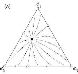
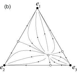
Figure 1: Dynamics of the extended AS model when the majority preference is present and the minority aversion is absent. We set $n=3$, $\beta=a$, $s_{1}=0.40$, $s_{2}=0.35$, and $s_{3}=0.25$. (a) $a=0.5$ and (b) $a=1.4$. Solid and open circles represent stable and unstable equilibria, respectively.

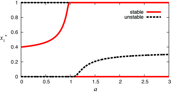
Figure 2: Bifurcation diagram for the extended AS model when the majority preference is present and the minority aversion is absent. The parameter values are equal to those used in Fig. 1 except that we vary $a$.

3.2 Case of minority aversion (i.e., $\beta=0$)

In this section, we set $\beta=0$ to analyze the case in which the majority preference is absent and the minority aversion is present. Substitution of Eq. (3) in Eq. (1) yields

$$\frac{dx_{i}}{dt} = s_{i}\sum_{j=1}^{n}x_{j}(1-x_{j})^{a}-(1-x_{i})^{a}x_{i}$$ (7)

$$= s_{i}\left<(1-x)^{a}\right>-(1-x_{i})^{a}x_{i}.$$

In contrast to the case of the majority preference (Sect. 3.1), the simplex spanned by $n^{\prime}$ ($2\leq n^{\prime}\leq n-1$) states is not invariant under the dynamics given by Eq. (7). Therefore, a state that once gets extinct may reappear. In this section, we numerically analyze Eq. (7) for $n=3$ and $n=4$. For general $n$, we analytically examine the special case in which $s_{i}$ is independent of $i$ in Sect. 3.3.

For $n=3$, the dynamics for various values of $a$ is shown in Fig. 3. We set $s_{1}=0.36$, $s_{2}=0.33$, and $s_{3}=0.31$. When $a$ is small $(a<1)$, there is a unique globally stable coexistence equilibrium in the interior (Fig. 3a). The three consensus equilibria $e_{1}$, $e_{2}$, and $e_{3}$ are unstable. At $a=1$, $e_{1}$, $e_{2}$, and $e_{3}$ change the stability such that they are stable beyond $a=1$ (Appendix B). Simultaneously, a saddle point bifurcates from each consensus equilibrium. The bifurcation occurs simultaneously for the three equilibria at $a=1$ irrespective of the values of $s_{1}$, $s_{2}$, and $s_{3}$. Slightly beyond $a=1$, the three consensus equilibria and the interior coexistence equilibrium are multistable (see Fig. 3b for the results at $a=1.3$). As $a$ increases, the attractive basin of the coexistence equilibrium becomes small, and that of each consensus equilibrium becomes large (see Fig. 3c for the results at $a=1.4$). At $a=a_{{\rm c}1}\approx 1.43$, the coexistence equilibrium that is stable for $a<a_{\rm c1}$ and the unstable interior equilibrium that bifurcates from $e_{i}$ at $a=1$, where $i$ corresponds to the largest $s_{i}$ value ($i=1$ in the present example), collide. This is a saddle-node bifurcation.

Numerically obtained $a_{\rm c1}$ values are shown in Fig. 4a for different values of $s_{1}$, $s_{2}$, and $s_{3}$. A point in the triangle in the figure specifies the values of $s_{1}$, $s_{2}$, and $s_{3}$ under the constraint $s_{1}+s_{2}+s_{3}=1$, $s_{i}>0$ ($1\leq i\leq 3$). It seems that $a_{\rm c1}$ is the largest when $s_{i}=1/3$ ($1\leq i\leq 3$). Figure 4 suggests that heterogeneity in $s_{i}$ makes $a_{\rm c1}$ smaller and hence makes the stable coexistence of the three states difficult. When $s_{i}\approx 1$ and $s_{j}\approx 0$ ($j\neq i$), we obtain $a_{\rm c1}\approx 1$.

When $a$ is slightly larger than $a_{{\rm c}1}$, there are two saddle points in the interior. In this situation, one of the three consensus equilibria, which depends on the initial condition, is eventually reached (Fig. 3d). However, the manner with which the triangular phase space is divided into the three attractive basins is qualitatively different from that in the case of the majority preference (Fig. 1b). In particular, in the present case of the minority aversion, even if $x_{1}$ is initially equal to 0, the consensus of state 1 (i.e., $e_{1}$) can be reached. This behavior never occurs in the case of the majority preference and less likely for a larger $a$ value in the case of the minority aversion (Fig. 3e).

The sizes of the attractive basins of the different equilibria are plotted against $a$ in Fig. 5a. Up to our numerical efforts with various initial conditions, we did not find limit cycles. A discrete jump in the basin size of the coexistence equilibrium is observed at $a_{\rm c1}\approx$ 1.43, reminiscent of the saddle-node bifurcation. Interestingly, the attractive basin of the consensus equilibrium $e_{1}$ is the largest just beyond $a_{\rm c1}$.

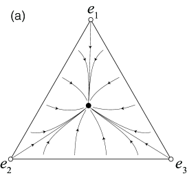
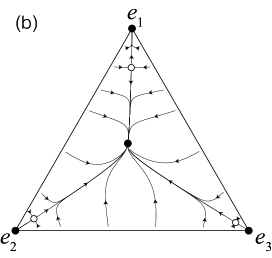
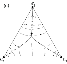
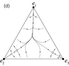
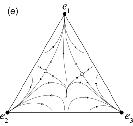
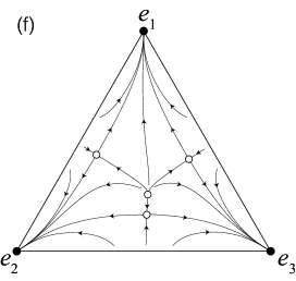
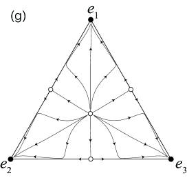
Figure 3: Dynamics of the extended AS model when the majority preference is absent and the minority aversion is present. We set $n=3$, $\beta=0$, $s_{1}=0.36$, $s_{2}=0.33$, and $s_{3}=0.31$. (a) $a=0.9$, (b) $a=1.3$, (c) $a=1.4$, (d) $a=1.5$, (e) $a=2.6$, (f) $a=2.9$, and (g) $a=10.0$.

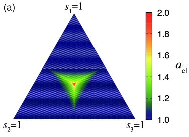
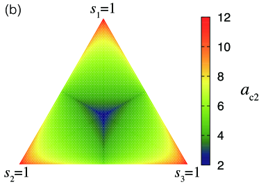
Figure 4: Dependence of (a) $a_{\rm c1}$ and (b) $a_{\rm c2}$ on $s_{1}$, $s_{2}$, and $s_{3}$ when the majority preference is absent and the minority aversion is present. A point in the triangle corresponds to a triplet ($s_{1}$, $s_{2}$, $s_{3}$), where $s_{1}+s_{2}+s_{3}=1$ and $s_{i}\geq 0$ ($1\leq i\leq 3$).

As $a$ increases further, the second saddle-node bifurcation occurs at $a=a_{\rm c2}\approx 2.81$, where an unstable node and a saddle point coappear (Fig. 3f). Logically, the sizes of the attractive basins could be discontinuous at $a=a_{\rm c2}$ because some initial conditions with small $x_{1}$ might be attracted to $e_{1}$ when $a$ is slightly smaller than $a_{\rm c2}$ and to $e_{2}$ or $e_{3}$ when $a$ is slightly larger than $a_{\rm c2}$. However, up to our numerical efforts, we did not observe the discontinuity, as implied by Fig. 5a.

Numerically obtained $a_{\rm c2}$ values are shown in Fig. 4b for different values of $s_{1}$, $s_{2}$, and $s_{3}$. Heterogeneity in $s_{i}$ makes $a_{\rm c2}$ larger. In addition, $a_{\rm c2}$ is equal to $a_{\rm c1}$ when $s_{1}=s_{2}=s_{3}=1/3$. In this symmetric case, the three saddle points simultaneously collide with the stable star node at $a=1$. Beyond $a=1$, the equilibrium that is the stable star node when $a<1$ loses its stability to become an unstable star node. The three saddle points move away from the unstable star node as $a$ increases. This transition can be interpreted as three simultaneously occurring transcritical bifurcations.

The unstable node that emerges at $a=a_{\rm c2}$ approaches $x_{i}^{*}=1/3$ ($1\leq i\leq 3$) in the limit $a\rightarrow\infty$, as shown in Appendix C. The three saddle points approach $(x_{1},x_{2},x_{3})=(1/2,1/2,0),(1/2,0,1/2)$, and $(0,1/2,1/2)$, as shown in Fig. 3g. This is a trivial consequence of the proof given in Appendix C. Therefore, the heterogeneity in $s_{i}$ does not play the role in the limit $a\to\infty$ such that the phase space is symmetrically divided into the three attractive basins corresponding to $e_{1}$, $e_{2}$, and $e_{3}$.

For $n=4$, the relationship between $a$ and the sizes of the attractive basins of the different equilibria is shown in Fig. 5b. The results are qualitatively the same as those for $n=3$ (Fig. 5a).

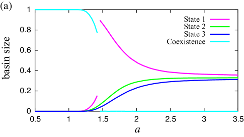
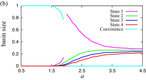
Figure 5: Sizes of the attractive basins for different equilibria when the majority preference is absent and the minority aversion is present. The lines with legend “State $i$” represent the basin size for the consensus equilibrium of state $i$. The lines with legend “Coexistence” represent the basin size for the coexistence equilibrium. (a) $n=3$, $\beta=0$, $s_{1}=0.36$, $s_{2}=0.33$, and $s_{3}=0.31$. (b) $n=4$, $\beta=0$, $s_{1}=0.28$, $s_{2}=0.26$, $s_{3}=0.24$, and $s_{4}=0.22$. We obtain $a_{{\rm c}1}\approx 1.43$ and $a_{{\rm c}2}\approx 2.81$ in (a) and $a_{{\rm c}1}\approx 1.91$ and $a_{{\rm c}2}\approx 3.29$ in (b). We calculate the sizes of the attractive basins as follows. First, we take the initial condition ($x_{1}$, $x_{2}$, $x_{3}$) $=$ ($0.01i$, $0.01j$, $0.01k$), where $i,j,k\geq 1$, $i+j+k=100$, for $n=3$ and ($x_{1}$, $x_{2}$, $x_{3}$, $x_{4}$) = ($0.05i$, $0.05j$, $0.05k$, $0.05\ell$), where $i,j,k,\ell\geq 1$, $i+j+k+\ell=20$, for $n=4$. Second, we run the dynamics starting from each initial condition until the trajectory converges. Third, we count fraction of the initial conditions that converge to each stable equilibrium.

3.3 Symmetric case

In the previous sections, we separately considered the effect of the majority preference (Sect. 3.1) and the minority aversion (Sect. 3.2). In this section, we examine the extended AS model when both effects can be combined. To gain analytical insight into the model, we focus on the symmetric case $s_{i}=s$ ($1\leq i\leq n$). Although normalization $\sum_{i=1}^{n}s_{i}=1$ leads to $s_{i}=1/n$, we set $s=1$ in this section to simplify the notation; $s$ just controls the time scale of the dynamics. Then, Eqs. (1) and (3) are reduced to

$$\frac{dx_{i}}{dt}=x_{i}^{\beta}\sum_{j=1,j\neq i}^{n}x_{j}(1-x_{j})^{a-\beta}-x_{i}(1-x_{i})^{a-\beta}\sum_{j=1,j\neq i}^{n}x_{j}^{\beta}.$$ (8)

Equation (8) implies that, regardless of the parameter values, there exist $n$ trivial consensus equilibria and symmetric coexistence equilibria of $n^{\prime}$ ($2\leq n^{\prime}\leq n$) states given by $x_{i}^{*}=1/n^{\prime}$, where $i$ varies over the $n^{\prime}$ surviving states arbitrarily selected from the $n$ states.

Owing to the conservation law $\sum_{i=1}^{n}x_{i}=1$, the dynamics are ($n-1$)-dimensional. The eigenvalues of the Jacobian matrix of the dynamics at the coexistence equilibrium containing the $n$ states are ($n-1$)-fold and given by $\left(\tfrac{1}{n}\right)^{\beta}\left(1-\tfrac{1}{n}\right)^{a-\beta-1}\left[(n-2)\beta+a-n+1\right]$, as shown in Appendix D. Therefore, the coexistence equilibrium is stable if and only if

$$(n-2)\beta+a-n+1<0.$$ (9)

Similarly, we show in Appendix B that the consensus equilibria are stable if and only if

$$a>1.$$ (10)

Coexistence equilibria of $n^{\prime}$ ($2\leq n^{\prime}\leq n-1$) states are always unstable (Appendix D).

Figure 6 is the phase diagram of the model in which the stable equilibria for given parameter values are indicated. The thin solid and dashed lines separating two phases are given by Eqs. (9) and (10), respectively. A multistable parameter region exists when $n\geq 3$; Eq. (9) is reduced to $a<1$ when $n=2$. When $n\geq 3$, the multistablity occurs except in the case of the pure majority preference (i.e., $\beta=a$). The multistable parameter region enlarges as $n$ increases.

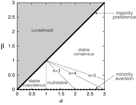
Figure 6: Phase diagram of the extended AS model when all the $s_{i}$ values are equal. The thin solid lines and the thin dashed line are given by Eqs. (9) and (10), respectively.

4 Discussion

We analyzed an extended AS model with $n$ states. We showed that the introduction of the minority aversion as compared to the majority preference changes the behavior of the model with $n\geq 3$ in two main aspects. First, different states stably coexist up to a larger $a$ value with the minority aversion than with the majority preference. Nevertheless, it should be noted that $a$ is the exponent associated with different quantities in the two cases (Eq. (3)). Second, the multistability of the consensus equilibria and the coexistence equilibrium is facilitated by the minority aversion and opposed by the majority preference. We verified that the main results also hold true in the case of more general transition rates than Eq. (3), expressed as $P_{ji}=s_{i}^{\gamma}(1-s_{j})^{1-\gamma}x_{i}^{\beta}(1-x_{j})^{a-\beta}$ (Appendix E).

Volovik and colleagues examined mean-field dynamics of a three-state opinion formation model with minority aversion Volovik2009EPL . Coexistence of at least two states occurs in their model even if a random choice term, equivalent to diffusive coupling, which the authors assumed, is turned off. This is because only the most minor state decreases in the number of individuals and the other two major states are equally strong in their model. In our model, the most major and second major states have different strengths in attracting individuals, and the coexistence equilibrium is stable only for small $a$.

Fu and Wang considered the combined effects of the majority preference and minority avoidance on coevolution of opinions and network structure Fu . They assumed that the majority preference is used for collective opinion formation and the minority avoidance guides network formation. They showed that segregated groups, each composed of individuals with the same opinion, evolve when the minority avoidance is dominantly used. The coexistence of multiple states owing to the segregation has also been shown in spatially extended AS models Patriarca1 ; Patriarca2 . We showed that coexistence of different states is facilitated by the minority aversion, not by the majority preference, and that stable coexistence occurs without segregation, or other spatial or network mechanisms.

Nowak and colleagues analyzed a replicator–mutator equation as a model of language evolution Nowak . They showed that coexistence of different grammars (i.e., states in our terminology) and a consensus-like configuration in which one grammar dominates the others are multistable when a learning parameter takes an intermediate value. If the learning is accurate, the consensus-like configuration becomes monostable. Our model and theirs differ in at least two aspects. First, the control parameter in our model is $a$, that is, the strength of the sum of the majority preference and minority aversion. Second, the stable coexistence in our model requires some minority aversion, whereas their model takes into account the majority preference but not the minority aversion.

Appendix A Unimodality of the Lyapunov function

We denote the Hessian of $V(\bm{x})$ by $H(V)$, which is an $(n-1)\times(n-1)$ matrix owing to the conservation law $\sum_{i=1}^{n}x_{i}=1$. We obtain

$$H_{ij}(V) = \frac{\partial^{2}V(\bm{x})}{\partial x_{i}\partial x_{j}}$$ (11)

$$= \begin{cases}a(1-a)\left(s_{i}x_{i}^{a-2}+s_{n}x_{n}^{a-2}\right)&(1\leq i=j\leq n-1),\\ a(1-a)s_{n}x_{n}^{a-2}&(1\leq i\neq j\leq n-1),\end{cases}$$

where $x_{n}=1-\sum_{i=1}^{n-1}x_{i}$ and $s_{n}=1-\sum_{i=1}^{n-1}s_{i}$. For any $\bm{x}$, $H(V)$ is positive (negative) definite for $a<1$ $(a>1)$ because

$$\bm{y}^{\mathrm{T}}H(V)\bm{y} = \sum_{i=1}^{n-1}a(1-a)s_{i}x_{i}^{a-2}y_{i}^{2}+\sum_{i=1}^{n-1}\sum_{j=1}^{n-1}a(1-a)s_{n}x_{n}^{a-2}y_{i}y_{j}$$ (12)

$$= a(1-a)\left[\sum_{i=1}^{n-1}s_{i}x_{i}^{a-2}y_{i}^{2}+s_{n}x_{n}^{a-2}\left(\sum_{i=1}^{n-1}y_{i}\right)^{2}\right]\gtrless 0\;\;\;\;\;\left(a\lessgtr 1\right),$$

for any $(n-1)$-dimensional nonzero vector $\bm{y}$. Therefore, $V(\bm{x})$ is strictly convex (concave) for $a<1$ ($a>1$) and hence has a unique global extremum at $\bm{x}^{*}$, which realizes the minimum (maximum) of $V(\bm{x})$.

Appendix B Eigenvalues of the Jacobian matrix in the consensus equilibria

On the basis of Eqs. (1) and (3), the $(n-1)\times(n-1)$ Jacobian matrix $(J_{ij})=(\partial\dot{x_{i}}/\partial x_{j})$ ($1\leq i,j\leq n-1$) is represented by

$$J_{ii}=\lim_{\begin{subarray}{c}x_{i}\to x_{i}^{*}\\ x_{k}=x_{k}^{*}\;\;(k\neq i)\end{subarray}}\left(\sum_{j=1,j\neq i}^{n}k_{ji}-l_{in}-\sum_{j=1,j\neq i}^{n}l_{ji}+k_{in}\right)$$ (13)

and

$$J_{ij}=\lim_{\begin{subarray}{c}x_{j}\to x_{j}^{*}\\ x_{k}=x_{k}^{*}\;\;(k\neq j)\end{subarray}}\left(l_{ij}-l_{in}-k_{ij}+k_{in}\right)\quad(i\neq j),$$ (14)

where

$$k_{ji} \equiv \beta s_{i}x_{i}^{\beta-1}x_{j}(1-x_{j})^{a-\beta},$$ (15)

$$l_{ji} \equiv s_{j}(1-x_{i})^{a-\beta-1}[1-(a-\beta+1)x_{i}]x_{j}^{\beta},$$ (16)

and

$$x_{n}=1-\sum_{i=1}^{n-1}x_{i}.$$ (17)

By exploiting symmetry, we examine the Jacobian matrix at the consensus equilibrium given by $x_{i}=0$ ($1\leq i\leq n-1$) and $x_{n}=1$. In this case, Eqs. (13) and (14) are reduced to

$$J_{ii}=as_{i}\lim_{x_{i}\to 0}x_{i}^{a-1}-s_{n}$$ (18)

and

$$J_{ij}=0,$$ (19)

respectively. Therefore, irrespective of the value of $\beta$, the eigenvalues of the Jacobian matrix, denoted by $\lambda_{i}$ ($1\leq i\leq n-1$), are given by

$$\lambda_{i}=J_{ii}=\begin{cases}-s_{n}&(a>1),\\ s_{i}-s_{n}&(a=1),\\ +\infty&(a<1).\end{cases}$$ (20)

Appendix C Coexistence equilibrium when $a\to\infty$

For general $n$, Eq. (7) implies that

$$\frac{(1-x_{i})^{a}x_{i}}{s_{i}}=\left<(1-x)^{a}\right>\quad(1\leq i\leq n)$$ (21)

is satisfied at the equilibrium. In particular, we obtain

$$\frac{(1-x_{i}^{*})^{a}x_{i}^{*}}{s_{i}}=\frac{(1-x_{j}^{*})^{a}x_{j}^{*}}{s_{j}}\quad(i\neq j).$$ (22)

Equation (22) leads to

$$\lim_{a\to\infty}\left(\log(1-x_{i}^{*})+\frac{\log x_{i}^{*}}{a}-\frac{\log s_{i}}{a}\right)=\lim_{a\to\infty}\left(\log(1-x_{j}^{*})+\frac{\log x_{j}^{*}}{a}-\frac{\log s_{j}}{a}\right).$$ (23)

Because the third term on each side of Eq. (23) is negligible, we obtain

$$\lim_{a\to\infty}\frac{1-x_{i}^{*}}{1-x_{j}^{*}}\left(\frac{x_{i}^{*}}{x_{j}^{*}}\right)^{\frac{1}{a}}=1.$$ (24)

The coexistence implies that $x_{i}^{*}$ and $x_{j}^{*}$ do not tend to 0 as $a\to\infty$. Therefore, Eq. (24) leads to $x_{i}^{*}=x_{j}^{*}$ in the limit $a\to\infty$. Therefore, $x_{i}^{*}=1/n$ ($1\leq i\leq n$).

Appendix D Eigenvalues of the Jacobian matrix in the coexistence equilibria in the symmetric case

On the basis of Eq. (8), the $(n-1)\times(n-1)$ Jacobian matrix $(J_{ij})=(\partial\dot{x_{i}}/\partial x_{j})$ is represented by Eqs. (13)–(17) with $s_{i}=1$ $(1\leq i\leq n)$. At the coexistence equilibrium given by $x_{i}^{*}=1/n$ ($1\leq i\leq n$), Eqs. (13) and (14) are reduced to

$$J_{ii}=n(k-l)=\left(\frac{1}{n}\right)^{\beta}\left(1-\frac{1}{n}\right)^{a-\beta-1}\left[(n-2)\beta+a-n+1\right]$$ (25)

and

$$J_{ij}=0,$$ (26)

respectively. Therefore, the eigenvalues of the Jacobian matrix are ($n-1$)-fold degenerate and given by

$$\lambda_{i}=J_{ii}=\left(\frac{1}{n}\right)^{\beta}\left(1-\frac{1}{n}\right)^{a-\beta-1}\left[(n-2)\beta+a-n+1\right]\quad(1\leq i\leq n-1).$$ (27)

By exploiting symmetry, we consider the coexistence equilibrium of $n^{\prime}$ states given by $x_{i}^{*}=0$ ($1\leq i\leq n-n^{\prime}$) and $x_{i}^{*}=1/n^{\prime}$ ($n-n^{\prime}+1\leq i\leq n$). In this case, Eqs. (13) and (14) with $s_{i}=1$ ($1\leq i\leq n$) are reduced to

$$J_{ii} = \begin{cases}\beta\left(1-\frac{1}{n^{\prime}}\right)^{a-\beta}\lim_{x_{i}\to 0}x_{i}^{\beta-1}-\left(\frac{1}{n^{\prime}}\right)^{\beta-1}&(1\leq i\leq n-n^{\prime}),\\ \left(\frac{1}{n^{\prime}}\right)^{\beta}\left(1-\frac{1}{n^{\prime}}\right)^{a-\beta-1}[(n^{\prime}-2)\beta+a-n^{\prime}+1]&(n-n^{\prime}+1\leq i\leq n-1),\end{cases}$$ (28)

$$J_{ij} = \begin{cases}\left(\frac{1}{n^{\prime}}\right)^{\beta+1}\left(1-\frac{1}{n^{\prime}}\right)^{a-\beta-1}[(n^{\prime}-2)\beta+a-n^{\prime}+1]&(n-n^{\prime}+1\leq i\leq n-1\\ \qquad+\left(\frac{1}{n^{\prime}}\right)^{\beta}-\beta\frac{1}{n^{\prime}}\left(1-\frac{1}{n^{\prime}}\right)^{a-\beta}\lim_{x_{j}\to 0}x_{j}^{\beta-1}&\quad\text{and }1\leq j\leq n-n^{\prime}),\\ 0&(\text{otherwise}).\end{cases}$$ (29)

The eigenvalues of the Jacobian matrix are the diagonal entries because the Jacobian matrix is a triangular matrix. Therefore, we obtain

$$\lambda_{i}=J_{ii} = \begin{cases}-\left(\frac{1}{n^{\prime}}\right)^{\beta-1}&(\beta>1),\\ \left(1-\frac{1}{n^{\prime}}\right)^{a-1}-1&(\beta=1),\\ +\infty&(\beta<1),\end{cases}$$ (30)

for $1\leq i\leq n-n^{\prime}$ and

$$\lambda_{i}=J_{ii}=\left(\frac{1}{n^{\prime}}\right)^{\beta}\left(1-\frac{1}{n^{\prime}}\right)^{a-\beta-1}[(n^{\prime}-2)\beta+a-n^{\prime}+1]$$ (31)

for $n-n^{\prime}+1\leq i\leq n-1$. Equations (30) and (31) imply that at least one eigenvalue is positive unless $a=\beta=1$. When $a=\beta=1$, all the eigenvalues are equal to zero.

Appendix E Analysis of a generalized model

Consider a variant of the extended AS model in which the transition rate given by Eq. (3) is replaced by

$$P_{ji}=s_{i}^{\gamma}(1-s_{j})^{1-\gamma}x_{i}^{\beta}(1-x_{j})^{a-\beta},$$ (32)

where $0\leq\gamma\leq 1$. Equation (3) is reproduced with $\gamma=1$. Here, the exponents $\gamma$ and $1-\gamma$ represent the strength of the preference for a strong state and the aversion to a weak state, respectively.

In the case of the majority preference (i.e., $\beta=a$), Eq. (1) with the transition rates given by Eq. (32) has $n$ trivial equilibria corresponding to the consensus and an interior equilibrium given by

$$x_{i}^{*}=\frac{\left(s_{i}^{-\gamma}(1-s_{i})^{1-\gamma}\right)^{\frac{1}{a-1}}}{\sum_{\ell=1}^{n}\left(s_{\ell}^{-\gamma}(1-s_{\ell})^{1-\gamma}\right)^{\frac{1}{a-1}}}.$$ (33)

There also exists a unique equilibrium composed of arbitrarily chosen $n^{\prime}$ states ($2\leq n^{\prime}\leq n-1$). The Lyapunov function is given by

$$V(\bm{x})=-\frac{\left<s^{\gamma}x^{a-1}\right>}{\left<(1-s)^{1-\gamma}\right>^{a}}.$$ (34)

$V(\bm{x})$ is a Lyapunov function because

$$\frac{d\left<s^{\gamma}x^{a-1}\right>}{dt} = \sum_{i=1}^{n}s_{i}^{\gamma}ax_{i}^{a-1}\frac{dx_{i}}{dt}$$ (35)

$$= a\sum_{i=1}^{n}s_{i}^{\gamma}x_{i}^{a-1}\left[s_{i}^{\gamma}x_{i}^{a}\left<(1-s)^{1-\gamma}\right>-(1-s_{i})^{1-\gamma}x_{i}\left<s^{\gamma}x^{a-1}\right>\right]$$

$$= a\left(\left<(s^{\gamma}x^{a-1})^{2}\right>\left<(1-s)^{1-\gamma}\right>-\left<s^{\gamma}x^{a-1}(1-s)^{1-\gamma}\right>\left<s^{\gamma}x^{a-1}\right>\right)$$

and

$$\frac{d\left<(1-s)^{1-\gamma}\right>}{dt} = \sum_{i=1}^{n}(1-s_{i})^{1-\gamma}\frac{dx_{i}}{dt}$$ (36)

$$= \sum_{i=1}^{n}(1-s_{i})^{1-\gamma}\left[s_{i}^{\gamma}x_{i}^{a}\left<(1-s)^{1-\gamma}\right>-(1-s_{i})^{1-\gamma}x_{i}\left<s^{\gamma}x^{a-1}\right>\right]$$

$$= \left<s^{\gamma}x^{a-1}(1-s)^{1-\gamma}\right>\left<(1-s)^{1-\gamma}\right>-\left<(1-s)^{2(1-\gamma)}\right>\left<s^{\gamma}x^{a-1}\right>$$

lead to

$$\frac{dV(\bm{x})}{dt} = -\frac{\frac{d}{dt}\left<s^{\gamma}x^{a-1}\right>}{\left<(1-s)^{1-\gamma}\right>^{a}}+\frac{a\left<s^{\gamma}x^{a-1}\right>\frac{d}{dt}\left<(1-s)^{1-\gamma}\right>}{\left<(1-s)^{1-\gamma}\right>^{a+1}}$$ (37)

$$= -\frac{a\left(\left<A^{2}\right>\left<B\right>^{2}-2\left<AB\right>\left<A\right>\left<B\right>+\left<A\right>^{2}\left<B^{2}\right>\right)}{\left<B\right>^{a+1}}$$

$$= -\frac{a\left<\left(A\left<B\right>-\left<A\right>B\right)^{2}\right>}{\left<B\right>^{a+1}}\;\;\;\;\leq 0,$$

where $A\equiv s^{\gamma}x^{a-1}$ and $B\equiv(1-s)^{1-\gamma}$.

We have no proof of the unimodality of $V(\bm{x})$. However, we numerically verified the unimodality for $n=3$. These results are the same as those obtained in the main text for $\gamma=1$ (Sect. 3.1).

For any $\beta$, the Jacobian matrix $(J_{ij})=(\partial\dot{x_{i}}/\partial x_{j})$ is given by Eqs. (13) and (14), where

$$k_{ji} \equiv \beta s_{i}^{\gamma}(1-s_{j})^{1-\gamma}x_{i}^{\beta-1}x_{j}(1-x_{j})^{a-\beta},$$ (38)

$$l_{ji} \equiv s_{i}^{\gamma}(1-s_{j})^{1-\gamma}(1-x_{j})^{a-\beta-1}[1-(a-\beta+1)x_{j}]x_{i}^{\beta},$$ (39)

and

$$x_{n}=1-\sum_{i=1}^{n-1}x_{i}.$$ (40)

In the consensus equilibrium given by $x_{i}=0$ ($1\leq i\leq n-1$) and $x_{n}=1$, Eqs. (13) and (14) are reduced to

$$J_{ii}=as_{i}^{\gamma}(1-s_{n})^{1-\gamma}\lim_{x_{i}\to 0}x_{i}^{a-1}-s_{n}^{\gamma}(1-s_{i})^{1-\gamma}$$ (41)

and

$$J_{ij}=0,$$ (42)

respectively. Therefore, the eigenvalues of the Jacobian matrix are given by

$$\lambda_{i}=J_{ii}=\begin{cases}-s_{n}^{\gamma}(1-s_{i})^{1-\gamma}&(a>1),\\ s_{i}^{\gamma}(1-s_{n})^{1-\gamma}-s_{n}^{\gamma}(1-s_{i})^{1-\gamma}&(a=1),\\ +\infty&(a<1),\end{cases}$$ (43)

and the consensus equilibrium is stable if $a>1$.

In the case of the minority aversion (i.e., $\beta=0$), when $n=3$, the sizes of the attractive basins for different equilibria for $\gamma=0$ and $\gamma=0.5$ are shown in Figs. 7a and 7b, respectively. The results are qualitatively the same as those for $\gamma=1$ (Fig. 5a).

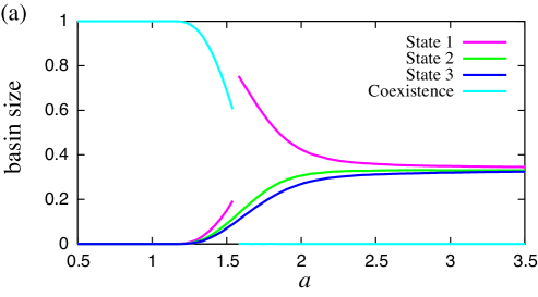
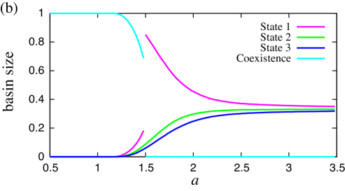
Figure 7: Sizes of the attractive basins for different equilibria when the majority preference is absent and the minority aversion is present in a generalized model. We set (a) $\gamma=0$ and (b) $\gamma=0.5$. We also set $n=3$, $\beta=0$, $s_{1}=0.36$, $s_{2}=0.33$, and $s_{3}=0.31$, the same parameter values as those used for Fig. 5a. We obtain $a_{{\rm c}1}\approx 1.57$ and $a_{{\rm c}2}\approx 2.56$ in (a) and $a_{{\rm c}1}\approx 1.50$ and $a_{{\rm c}2}\approx 2.69$ in (b). The procedure for calculating the basin size is described in the caption of Fig. 5.

References

- (1) Abrams, D.M., Strogatz, S.H.: Modelling the dynamics of language death. Nature 424, 900 (2003)
- (2) Abrams, D.M., Yaple, H.A., Wiener, R.J.: Dynamics of social group competition: Modeling the decline of religious affiliation. Phys. Rev. Lett. 107, 088701 (2011)
- (3) Castellano, C., Fortunato, S., Loreto, V.: Statistical physics of social dynamics. Rev. Mod. Phys. 81, 591–646 (2009)
- (4) Castelló, X., Eguíluz, V.M., San Miguel, M.: Ordering dynamics with two non-excluding options: bilingualism in language competition. New J. Phys. 8, 308 (2006)
- (5) Castelló, X., Toivonen, R., Eguíluz, V.M., Saramäki, J., Kaski, K., San Miguel, M.: Anomalous lifetime distributions and topological traps in ordering dynamics. Europhys. Lett. 79, 66006 (2007)
- (6) Chapel, L., Castelló, X., Bernard, C., Deffuant, G., Eguíluz, V.M., Martin, S., San Miguel, M.: Viability and resilience of languages in competition. PLoS ONE 5, e8681 (2010)
- (7) Chen, P., Redner, S.: Majority rule dynamics in finite dimensions. Phys. Rev. E 71, 036101 (2005)
- (8) Chen, P., Redner, S.: Consensus formation in multi-state majority and plurality models. J. Phys. A 38, 7239–7252 (2005).
- (9) de Oliveira, M.J.: Isotropic majority-vote model on a square lattice. J. Stat. Phys. 66, 273–281 (1992)
- (10) Fu, F., Wang, L.: Coevolutionary dynamics of opinions and networks: From diversity to uniformity. Phys. Rev. E 78, 016104 (2008)
- (11) Galam, S.: Majority rule, hierarchical structures, and democratic totalitarianism: A statistical approach. J. Math. Psych. 30, 426–434 (1986)
- (12) Galam, S.: Application of statistical physics to politics. Physica A 274, 132–139 (1999)
- (13) Galam, S.: Minority opinion spreading in random geometry. Eur. Phys. J. B 25, 403–406 (2002)
- (14) Hofbauer, J., Sigmund, K.: Evolutionary Games and Population Dynamics. Cambridge University Press, Cambridge (1998)
- (15) Krapivsky, P.L., Redner, S.: Dynamics of majority rule in two-state interacting spin systems. Phys. Rev. Lett. 90, 238701 (2003)
- (16) Lambiotte, R., Ausloos, M., Hołyst, J.A.: Majority model on a network with communities. Phys. Rev. E 75, 030101(R) (2007)
- (17) Lambiotte, R.: How does degree heterogeneity affect an order-disorder transition? Europhys. Lett. 78, 68002 (2007)
- (18) Lambiotte, R., Ausloos, M.: Coexistence of opposite opinions in a network with communities. J. Stat. Mech., P08026 (2007)
- (19) Lambiotte, R., Saramäki, J., Blondel, V.D.: Dynamics of latent voters. Phys. Rev. E 79, 046107 (2009)
- (20) Li, C., Hu, Y., Sun, L.: An improved Abrams-Strogatz model based protocol for agent competition and strategy designing. In: Wang, Y., Li, T. (eds.) Foundations of Intelligent Systems. Advances in Intelligent and Soft Computing, vol. 122, pp. 151–158. Springer, Berlin (2012)
- (21) Li, P.-P., Zheng, D.-F., Hui, P.M.: Dynamics of opinion formation in a small-world network. Phys. Rev. E 73, 056128 (2006)
- (22) Liggett, T.M.: Interacting Particle Systems. Springer, New York (1985)
- (23) Minett, J.W., Wang, W.S-Y.: Modelling endangered languages: The effects of bilingualism and social structure. Lingua 118, 19–45 (2008)
- (24) Mira, J., Paredes, Á.: Interlinguistic similarity and language death dynamics. Europhys. Lett. 69, 1031–1034 (2005)
- (25) Mira, J., Seoane, L.F., Nieto, J.J.: The importance of interlinguistic similarity and stable bilingualism when two languages compete. New J. Phys. 13, 033007 (2011)
- (26) Mobilia, M., Redner, S.: Majority versus minority dynamics: Phase transition in an interacting two-state spin system. Phys. Rev. E 68, 046106 (2003)
- (27) Nowak, M.A., Komarova, N.L., Niyogi, P.: Evolution of universal grammar. Science 291, 114–118 (2001)
- (28) Patriarca, M., Leppänen, T.: Modeling language competition. Physica A 338, 296–299 (2004)
- (29) Patriarca, M., Heinsalu, E.: Influence of geography on language competition. Physica A 388, 174–186 (2009)
- (30) Pinasco, J.P., Romanelli, L.: Coexistence of languages is possible. Physica A 361, 355–360 (2006)
- (31) Tessone, C.J., Toral, R., Amengual, P., Wio, H.S., San Miguel, M.: Neighborhood models of minority opinion spreading. Eur. Phys. J. B 39, 535–544 (2004)
- (32) Toivonen, R., Castelló, X., Eguíluz, V.M., Saramäki, J., Kaski, K., San Miguel, M.: Broad lifetime distributions for ordering dynamics in complex networks. Phys. Rev. E 79, 016109 (2009)
- (33) Vazquez, F., Castelló, X., San Miguel, M.: Agent based models of language competition: macroscopic descriptions and order-disorder transitions. J. Stat. Mech., P04007 (2010)
- (34) Volovik, D., Mobilia, M., Redner, S.: Dynamics of strategic three-choice voting. Europhys. Lett. 85, 48003 (2009)
- (35) Wang, W.S-Y., Minett, J.W.: The invasion of language: emergence, change and death. Trends Ecol. Evol. 20, 263–269 (2005)