Microscopically Computing Free-energy Profiles and Transition Path Time of Rare Macromolecular Transitions

Abstract

We introduce a rigorous method to microscopically compute the observables which characterize the thermodynamics and kinetics of rare macromolecular transitions for which it is possible to identify a priori a slow reaction coordinate. In order to sample the ensemble of statistically significant reaction pathways, we define a biased molecular dynamics (MD) in which barrier-crossing transitions are accelerated without introducing any unphysical external force. In contrast to other biased MD methods, in the present approach the systematic errors which are generated in order to accelerate the transition can be analytically calculated and therefore can be corrected for. This allows for a computationally efficient reconstruction of the free-energy profile as a function of the reaction coordinate and for the calculation of the corresponding diffusion coefficient. The transition path time can then be readily evaluated within the Dominant Reaction Pathways (DRP) approach. We illustrate and test this method by characterizing a thermally activated transition on a two-dimensional energy surface and the folding of a small protein fragment within a coarse-grained model.

I Introduction

The recent developments in single-molecule optical- and force- spectroscopy allow to experimentally characterize the thermodynamics and kinetics of many fundamental biomolecular reactions to an unprecedented level of accuracy. For example, pulling experiments based on optical tweezers tweezers or atomic-force microscopy AFM can provide the full free-energy profile of biopolymers as a function of their end-to-end distance reconstr , while the single-molecule Föster Resonance Energy Transfer spectroscopy yields the reaction rate FRET and, very recently, the transition path time (TPT) TPT .

The possibility of measuring these observables poses the challenge to predict their dynamics from microscopic atomistic simulations. Unfortunately, the MD algorithms are very inefficient to this purpose, because they require to simulate time intervals which are exponentially long in the free-energy barrier.

These limitations have motivated the development of alternative theoretical frameworks to investigate the free energy landscape eq1 ; eq2 ; eq3 and reaction kinetics properties neq1 ; neq2 ; neq3 ; neq4 ; neq5 ; neq6 ; neq7 ; neq8 ; neq9 ; neq10 of activated reactions. Some of these methods — such as e.g. the meta-dynamics approach eq1 — involve a suitable choice of a set of reaction coordinates which are used to bias and accelerate the exploration of the energy landscape. By contrast, methods like transition interface sampling neq8 , milestoning neq9 or dynamics Monte Carlo neq10 sample directly the space of reactive pathways, without introducing a bias on the dynamics. On the other hand, these methods are in general computationally quite costly.

In a recent work, a variant of the Dominant Reaction Pathway (DRP) method DRP0 ; DRP1 ; DRP2 has been developed DRPpnas , which generates statistically significant protein folding pathways by combining an accelerated MD algorithm ratchetMD with a path-integral based variational approach. Using the accelerated MD, several hundreds of folding trajectories for single-domain proteins of typical size can be generated in just a few hundreds of CPU hours. The trial paths are then ranked in terms of their statistical weight in the (unbiased) over-damped Langevin dynamics, and the most probable (i.e. least biased) trajectories among them are identified. This way, many of such so-called dominant reaction pathways, each corresponding to a different initial condition, have been computed for a WW protein domain using a realistic force field DRPpnas . These paths were found to agree very well with those obtained by Shaw and co-workers within the same force field, by means of ultra-long MD simulations on the Anton special-purpose machine Anton .

The high efficiency of the DRP method comes from the fact that its computational time does not scale exponentially with the free-energy barriers. By this method it is now possible to atomistically study the dynamics of polypeptides with realistic size and kinetics, and even simulate the folding of complex knotted proteins knotted .

The main limitation of this approach is that, since the accelerated dynamics used to generate the ensemble of reaction pathways breaks microscopic reversibility, it cannot be used to directly compute kinetic and thermodynamic observables. Due to this problem, to date the DRP method has been used only to investigate the reaction mechanism, for example by characterizing the transition state ensemble.

In this work, we overcome this limitation. We devise a rigorous scheme to compute the transition path time and evaluate the potential of mean-force of a previously determined slowly-evolving collective coordinate (CC). The method is based on a new type of accelerated MD algorithm, herby called hindered molecular dynamics (hMD). In contrast to other methods, in the hMD algorithm, no external force is introduced to speed up the reaction. In addition, the effect of the bias on the evolution of a slow reaction coordinate can be rigorously and analytically computed, hence can be corrected for. As a result, it is possible to extract the potential of mean-force and the diffusion coefficient of the reaction coordinate from a set of suitable averages evaluated over the reactive trajectories obtained from the biased dynamics. Once these quantities have been determined, the transition path time can be easily computed employing the DRP formalism.

The paper is organized as follows. In the next section we introduce the hMD dynamics and show how to extract the potential of mean-force and the diffusion constant of a slow reaction coordinate. In section III we discuss how to compute the transition path time in the DRP formalism. Section IV provides two illustrative applications to systems of increasing complexity. Finally, results and conclusions are summarized in section V.

II Computing the potential of mean-force and the diffusion coefficient of a CC from hMD simulations

Let us begin by considering the over-damped Langevin equation which mimics the microscopic dynamics of the molecule in a solvent. In the so-called Ito calculus this equation is defined as:

$$x_{i+1}=x_{i}-(\Delta t/\gamma)\nabla U(x_{i})+\sqrt{2D\Delta t}~{}\eta_{i},$$ (1)

where $\gamma$ is the viscosity, $D=\frac{k_{B}T}{\gamma}$ is the diffusion coefficient, $x_{i}$ is the point in the $3N$-dimensional configuration space visited at the $i-$th time step, $U(x)$ is the potential energy and $\eta(t)$ is a stochastic variable sampled from a Gaussian distribution with with zero average and unitary variance. The high-friction limit which underlies the over-damped Langevin Eq. (1) is appropriate for many systems of biophysical interest. For example, in proteins, the effects of the acceleration affects the dynamics only at time scales smaller than few fractions of ps pitard .

We now introduce the hMD, which is closely related to the ratchet-and-pawl MDratchetMD used to generate trial paths in our previous protein folding DRP calculations DRPpnas . The main difference between the two algorithms is that, in the hMD, no unphysical external force is introduced to disfavor fluctuations in the direction of the reactant. Instead, when the system tries to evolve backwards along a reaction coordinate, the dynamics is slowed down by increasing the viscosity and the decreasing the heat-bath temperature.

Namely, denoting with $z(x)$ a configuration-dependent CC —assumed for definiteness to monotonically increase from the reactant to the product—, the hMD is defined by the following stochastic differential equation:

$$x_{i+1} = \theta\left[z(x_{i+1})-z(x_{i})\right]~{}\left(x_{i}-\frac{\Delta t}{\gamma}\nabla U(x_{i})+\sqrt{2D\Delta t}\eta_{i}\right)$$

$$+ \theta\left[z(x_{i})-z(x_{i+1})\right]~{}\left(x_{i}-\frac{\Delta t}{\xi\gamma}\nabla U(x_{i})+\frac{1}{\xi}\sqrt{2D\Delta t}\eta_{i}\right),$$

where $\xi>1$ is called the hindering coefficient.

By scoring the trajectories generated by the hMD (II) according to the path probability of the unbiased Langevin dynamics (1) one can efficiently obtain an ensemble of statistically representative reaction pathways, see Ref. DRPpnas . Unfortunately, the time intervals of the hMD (II) are not physically meaningful and dominant pathways alone do not allow to compute free-energy differences.

In order to overcome this problem and establish the connection with kinetics and thermodynamics our strategy is to analyze the average time evolution of some slow reaction coordinate $Q$. In general, such a collective variable does not necessarily need to coincide with the biasing variable $z$, but can be related to it by a constant scaling factor, which produces a rescaling of the diffusion coefficient.

In the limit in which the spontaneous time evolution of the CC $Q$ very slow compared to that of all microscopic degrees of freedom, its (unbiased) dynamics can be described by an effective over-damped Langevin equation:

$$Q_{i+1}=Q_{i}-(\Delta t/\gamma_{Q})~{}G^{\prime}(Q_{i})+\sqrt{2k_{B}T\Delta t/\gamma_{Q}}~{}\eta_{i},$$ (3)

where $\gamma_{Q}$ and $D_{Q}=k_{B}T/\gamma_{Q}$ the respectively the viscosity and the diffusion coefficient of the CC. In the following we restrict to the case in which the diffusion constant is assumed to be state independent (white noise). The generalization to colored noise is possible but it requires a careful choice of the stochastic calculus, and will not be considered in this first work.

In an hMD simulation, any time the system evolves towards a smaller value of the $Q$ (hence of $z$), the dynamics is slowed down by the same rescaling of the diffusion coefficient and temperature of the underlying microscopic dynamics. Hence, the equation of motion of $Q$ in a hMD simulation is given by:

$$Q_{i+1}-Q_{i} = \left(-\frac{\Delta t}{\gamma_{Q}}~{}G^{\prime}(Q_{i})+\sqrt{2D_{Q}\Delta t}~{}\eta_{i}\right)$$

$$\cdot \left\{1+\left(\frac{1}{\xi}-1\right)\theta\left[\sqrt{\frac{\Delta t}{2\gamma_{Q}k_{B}T}}~{}G^{\prime}(Q_{i})-\eta_{i}\right]\right\},$$

where the role of the step-function is to hinder the dynamics when the fluctuation would drive the reaction backwards.

From the stochastic differential Eq. (II) it is immediate to compute the probability for the system to evolve from a configuration with CC $Q_{i}$ to one with CC $Q_{i+1}$, in a elementary step $\Delta t$ of hMD simulation:

$$\mathcal{P}(Q_{i+1},\Delta t|Q_{i})=\mathcal{N}~{}\left(\xi e^{\frac{-\xi^{2}(\Delta Q+\frac{\Delta t}{\xi\gamma_{Q}}G^{\prime}(Q_{i}))^{2}}{4D_{Q}\Delta t}}\theta\left[-\Delta Q\right]\right.$$

$$\left.+e^{\frac{-(\Delta Q+\frac{\Delta t}{\gamma_{Q}}G^{\prime}(Q_{i}))^{2}}{4D_{Q}\Delta t}}~{}\theta\left[\Delta Q\right]\right),$$ (5)

where $\Delta Q\equiv Q_{i+1}-Q_{i}$ and $\mathcal{N}=\sqrt{\frac{\gamma_{Q}}{4\pi~{}\Delta t~{}k_{B}T}}$.

Using this equation we compute the average infinitesimal displacement of the CC $Q$ in a time interval $\Delta t$ of hMD, starting from configurations in which the CC takes a value $Q$:

$$\langle\Delta Q(Q)\rangle_{hMD}=\sqrt{\frac{\Delta tk_{B}T}{\pi\gamma_{Q}}}\frac{\xi-1}{\xi}-\frac{\Delta t}{2\gamma_{Q}}G^{\prime}(Q)\frac{1+\xi}{\xi}+\ldots$$ (6)

Similarly, the average square displacement $\langle\Delta Q^{2}(Q)\rangle_{hMD}$ reads:

$$\langle\Delta Q^{2}(Q)\rangle_{hMD} = \frac{\Delta tk_{B}T}{\gamma_{Q}}~{}\frac{1+\xi^{2}}{\xi^{2}}+\ldots$$ (7)

In both equations (6) and (7) the dots denote corrections of order $\Delta t^{3/2}$. If the biasing coordinates is defined in such a way to decrease (rather than increase) from the reactant to the product, the first term in the right-hand-side of Eq. (6) changes sign. The averages in Eq.s (6) and (7) can be efficiently evaluated, hence allowing to determine $\gamma_{Q}$ and $G(Q)$.

III Computing the Transition Path Time

In the previous section we have discussed how it is possible to compute the potential of mean-force $G(Q)$ and the diffusion coefficient $D_{Q}$, by evaluating averages over microscopic trajectories obtained in the hMD. We now show that, once these quantities have been determined, it is possible to restore the correct time scales in the calculated reactive trajectories, by applying the DRP formalism to the stochastic projected dynamics of the CC defined in Eq. (3).

The starting point of the DRP approach is the path integral representation of the conditional probability of going from $Q_{i}$ to $Q_{f}$ in time $t$:

$$\mathcal{P}(Q_{f},t|Q_{i})=e^{-\frac{G(Q_{f})-G(Q_{i})}{2k_{B}T}}~{}\int_{Q_{i}}^{Q_{f}}\mathcal{D}Q~{}e^{-S_{eff}[Q]},$$ (8)

where

$$S_{eff}[Q]=\int_{0}^{t}d\tau\left(\frac{\dot{Q}^{2}}{4D_{Q}}+V_{eff}[Q]\right)$$ (9)

is called the effective action and

$$V_{eff}(Q)=\frac{D_{Q}}{4(k_{B}T)^{2}}(|G^{\prime}(Q)|^{2}-2k_{B}TG^{\prime\prime}(Q))$$ (10)

is called the effective potential. The DRP equations result from analyzing the path integral (8) in saddle-point approximation. The saddle-point paths (called the dominant reaction pathways) are the functional minima of the effective action. Hence, they obey the equation of motion

$$\ddot{Q}=2D_{Q}V^{\prime}_{eff}(Q)~{}$$ (11)

and conserve the effective energy $E_{eff}\equiv\frac{\dot{Q}^{2}}{4D_{Q}}-V_{eff}[Q].$

As discussed in detail Ref.s DRP2 ; DRPfluct the saddle-point paths which are relevant in the description of thermal activation are those which leave the reactant and reach the product with (nearly) vanishing velocity. This observation implies

$$E_{eff}\sim~{}-V_{eff}(Q_{i})~{}\sim\frac{1}{2\gamma}G^{\prime\prime}(Q_{i}),$$ (12)

where we have used the fact the initial configuration $Q_{i}$ is in the vicinity of a free energy minimum. On the other hand, outside the (meta-) stable thermodynamical states, the effective potential is dominated by its force contribution,

$$V_{eff}(Q)\sim 1/(4k_{B}T\gamma_{Q})|G^{\prime}(Q)|^{2}.$$ (13)

Hence, in the transition region $E_{eff}/V_{eff}(Q)\sim o(k_{B}T)$.

The definition of effective energy immediately yields the time at which any given intermediate value $Q$ of the CC, located between the reactant $Q_{R}$ and the product $Q_{P}$, is visited by during a reaction DRP0 ; DRP2 :

$$t(Q)=\int_{Q_{R}}^{Q}\frac{dQ}{\sqrt{4D_{Q}(E_{eff}+V_{eff}[\bar{Q}])}}.$$ (14)

This equation can also be used compute the time at which the microscopic configurations in the dominant trajectories are reached, by imposing $t(x)\simeq t(Q(x))$. In particular, Eq. (14) provides an estimate of the TPT, which is obtained simply by setting $Q=Q_{P}$ and $E_{eff}\sim~{}-V_{eff}(Q_{R})$.

III.1 Transition path time for crossing a harmonic barrier

It is useful to discuss the TPT calculation within the simple harmonic approximation of a single free-energy barrier, which allows for an analytic treatment. In this case, the effective potential $V_{eff}(Q)$ is also a harmonic function and reads

$$V_{eff}(Q)\simeq\frac{\alpha^{2}}{4k_{B}T\gamma_{Q}}\cdot(Q-Q_{TS})^{2}+\frac{\alpha}{2\gamma_{Q}},$$ (15)

where $Q_{TS}$ identifies the transition state and $\alpha\equiv G^{\prime\prime}(Q_{TS})$.

In an harmonic barrier, the transitions which involve overcoming of an energy barrier $\Delta G$ are those initiated by a point $Q_{i}$ such that $|Q_{TS}-Q_{i}|=\sqrt{\frac{2\Delta G}{\alpha}}$. Hence, Eq. (14) immediately gives

$$t_{TPT}=\frac{\gamma}{\alpha}\ln\left[\frac{\left(\sqrt{2\Delta G\alpha}+2\sqrt{k_{B}T[E_{eff}+\frac{\alpha}{2}(1+\frac{\Delta G}{k_{B}T})}]\right)^{2}}{2k_{B}T(\alpha+2E_{eff})}\right]$$ (16)

Finally, retaining only the leading-order in the expansion in powers of the thermal energy $k_{B}T$ and recalling that $E_{eff}/V_{eff}\sim o(k_{B}T)$ we arrive to the final simple result,

$$t_{TPT}=\frac{\gamma}{\alpha}\ln\left[4\Delta G/(k_{B}T)\right],$$ (17)

which is close to the estimate obtained by Szabo, $t_{TPT}\simeq\frac{\gamma}{\alpha}\ln[3\Delta G/(k_{B}T)]$. It should be emphasized however that Eq. (14) generalizes this estimate beyond the harmonic approximation and the leading-order in the low-temperature expansion.

IV Illustrative applications and Validation

For illustration and validation purposes, in the remaining of this work we apply and test our method to characterize two reaction of increasing complexity. We begin by considering a simple two-dimensional toy model which can be straightforwardly implemented and for which analytic solution for the potential of mean-force exist.

Next, we use our method to study a protein folding reaction within a coarse-grained representation of the polypeptide chain. In such a model, the folding reaction can be simulated directly by integrating the equation of motion and the results can be used to assess the accuracy of our method.

IV.1 Diffusion on two-dimensional funneled potential

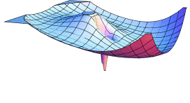
We consider the over-damped Langevin diffusion of a point-particle in the two-dimensional funneled energy surface shown in Fig.1, which is given by the potential:

$$U(x,y) = \frac{-A_{1}\sigma_{1}^{2}}{((x^{2}+y^{2})+\sigma_{1}^{2})^{2}}+\frac{A_{2}\sigma_{1}^{2}}{((x^{2}+y^{2})+\sigma_{2}^{2})}$$

$$+\omega^{2}(x^{2}+y^{2})^{2}+B\sin^{2}\left(\frac{\phi}{2}\right),\quad\phi=\arctan\left(y/x\right),$$

with $A_{1}=20$, $A_{2}=10$, $\sigma_{1}=1$, $\sigma_{2}=5$, $\omega=0.02$ and $B=10.$ As shown in Fig. 1 this model contains a stable state at the origin and meta-stable state at some finite distance from the bottom of the funnel and $\phi\simeq 0$. For $k_{B}T=1$, the barrier-crossing transition from the meta-stable to the stable state is thermally activated. The only slow coarse coordinate in this system is the distance of the particle from the origin, $R=\sqrt{x^{2}+y^{2}}$ and the dominant reaction pathways are straight lines connecting the different initial conditions in the meta-stable state to the origin. By contrast, a typical Langevin trajectory spends a large time in the metastable state, performs a barrier crossing transition and eventually lands in the stable state.

Figure 1: (Color online) The energy surface of the two-dimensional toy model used to validate the method.

The mean first-passage-time through the transition state, obtained from the Langevin simulations is $\langle t_{FPT}\rangle_{MD}=532\pm 40$ (units in which $\gamma\equiv 1$). The mean TPT can be calculated by measuring the length of an ensemble of Langevin trajectories which are started at the edge of the reactant –arbitrarily defined by the condition $R_{R}=5$– and are terminated once the particle reaches the edge of the product– identified by the condition $R_{P}=0.5$. Accumulating statistics only on the trajectories which do not visit the reactant before reaching the product we find $\langle t_{TPT}\rangle_{MD}=2.65\pm 0.02$.

Figure 2: (Color online) Upper panel: $\langle\Delta R^{2}(R)\rangle$ in the toy model, evaluated in hMD (circles) and MD (squares) simulations. Lower panel: $\langle\Delta R(R)\rangle$ in hMD simulations. All quantities are in computer units.

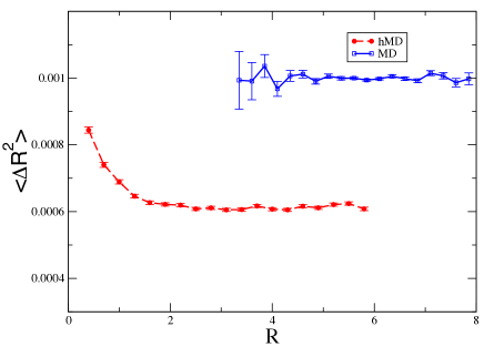
We now use Eq.s (6) and (7) to reconstruct the free energy landscape as a function of the CC $z=R$. This is done by running hMD simulations which bias the dynamics towards smaller and smaller distances from the origin, according to the algorithm given in Eq. (II). With a hindering coefficient $\xi=2$, generating a barrier crossing event requires simulating a time interval of about $0.4$, which is a factor $10^{3}$ times smaller than the mean-first-passage time. hMD trajectories are functionally close to the dominant reaction pathway, i.e. to the straight radial line with $\phi=0$.

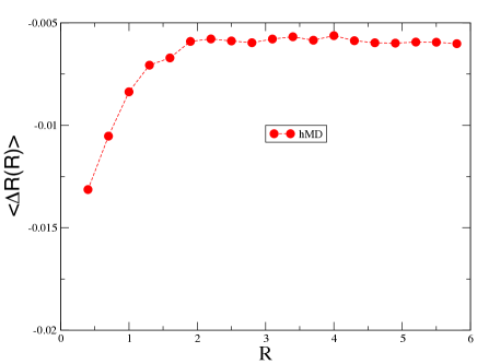
According to our method, the first step towards reconstructing the free-energy surface consists in evaluating the friction coefficient for the CC used in the hMD, by means of Eq. (7). Fig. 2 shows $\langle\Delta R^{2}(R)\rangle$ evaluated in the hMD simulation with an elementary time interval $\Delta t=0.0005$. As predicted by Eq. (7), this curve is flat almost everywhere. A weak dependence on $R$ is observed for $R\lesssim 2$, and is due to the fact that in the high-force region inside the funnel, gradient-dependent corrections to Eq. (7) which are higher order in $\Delta t$ become relevant. From a fit of the flat region, knowing that $\xi=2$, one obtains the correct result $\gamma_{R}\simeq 1$. To assess the validity of this calculation, in Fig. 2 we also show the same average evaluated in standard (i.e. unbiased) MD simulations. According to Einstein’s law this average should be equal $\frac{2\Delta tk_{B}T}{\gamma_{R}}$, which allows to confirm the result obtained from hMD.

Finally, knowing $\xi$ and having determined $\gamma_{R}$, it is possible to use Eq. (6) to extract the mean-force $G^{\prime}(R)$ from the average displacement $\langle\Delta R(R)\rangle$ shown in Fig. 2, hence to reconstruct $G(R)$. The calculated free-energy is shown in Fig. 3, where it is compared with the exact analytic result, $G(R)=U(R)-k_{B}T\log\frac{R}{R_{0}}$, – here, $R_{0}$ is the arbitrary reference point—. The agreement between the two curves is quantitative.

Figure 3: (Color online) Comparison between exact (solid line) and calculated (circles) free-energy profile as a function of the CC $R$. The dotted line represents the potential energy as a function of the coordinate $R$, evaluated along the radial line with polar coordinate $\phi=0$. The dot-dashed line shows the DRP time at which each value of $R$ is assumed.

The TPT estimated using the DRP equation (14), setting the $E_{eff}=-V_{eff}(R_{m})$ –where $R_{m}$ is the minimum free-energy distance in the meta-stable state— gives $t_{TPT}^{DRP}\simeq 3.4$. This number is not far from the average $\langle t_{TPT}\rangle_{MD}=2.65\pm 0.02$, obtained by MD simulations. In contrast, Szabo’s formula, which relies on the harmonic approximation and low-temperature expansion, gives $t_{TPT}^{Sz}=0.8$, which is off by a factor 3. This discrepancy suggest that temperature effects and specific curvature of the energy surface at the transition state can give significant corrections to the TPT.

IV.2 The folding of a poly-petide chain

To further assess the accuracy and computational efficiency of our method, we apply it to study a conformational reaction which resembles most of the difficulties which are encountered in macromolecular systems: the folding of the 16 amino-acid C-terminus of protein GB1, whose native state is shown in the inset of Fig.4.

To allow for a direct comparison with the result of standard MD simulations, we adopt the coarse-grained representation introduced in Ref. DRPlonardi . In such an approach, the explicit degrees of freedom individual amino-acids and the energy function is a sum of pair-wise interactions:

$$U = \frac{1}{2}\sum_{k}k(x_{k+1}-x_{k}|-a)^{2}+\sum_{i<j}4\epsilon\left[A_{ij}\left(\frac{\sigma}{|x_{j}-x_{i}|}\right)^{12}\right.$$ (19)

$$\left.-(G_{ij}+B_{ij})~{}\left(\frac{\sigma}{|x_{j}-x_{i}|}\right)^{6}\right]$$

where $x_{i}$ denotes the position of the $i-$th residue, $a=0.38$ nm, $k=3000~{}\textrm{kJ mo}l^{-1}\textrm{nm}^{-2}$, $\epsilon=5~{}\textrm{kJ mol}^{-1}$, and $\sigma=0.3~{}$nm. $G_{ij}$ is the matrix of native contacts, i.e. $G_{ij}$ is set to $1$ if the distance between the residues $i$ and $j$ in the crystal native conformation is less than $0.65$ nm, and $0$ otherwise (Go-type model, go ). The coefficients $A_{ij}$ and $B_{ij}$ are introduced in order to account for the hydro-philic (-phobic) character of the amino-acids, as in the so-called HP model HPmodel .

Figure 4: (Color online) Potential of mean-force as a function of the fraction of native contacts for the C-terminal of protein GB1 (the native structure shown in the insert).

Namely, we set

• $A_{ij}=1$ and $B_{ij}=1$, for pairs in which both amino-acids are hydrophobic

• $A_{ij}=\frac{2}{3}$ and $B_{ij}=-1$, for pairs in which one of the amino-acids is polar

• $A_{ij}=1$ and $B_{ij}=0$ if one of the residues is GLY, which is hydrophobically neutral.

Such non-native interactions introduce ruggedness in the energy landscape, making simulations more challenging than in the purely native-centric model.

Figure 5: (Color online) The time evolution of the fraction of native contacts $Q$ of the poly-peptide obtained from a long Langevin simulation with reversible folding-unfolding events (upper panel). The lower panel shows in detail the evolution of this variable along a typical folding event. The integration of the (Ito) Langevin equation (1) was performed at the nominal temperature of $T=200$ K, with an integration time step $\Delta t=0.01$ps and a viscosity $\gamma=2000$ amu ps^-1.

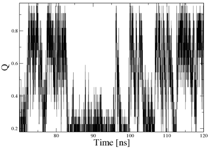
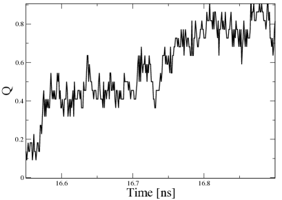
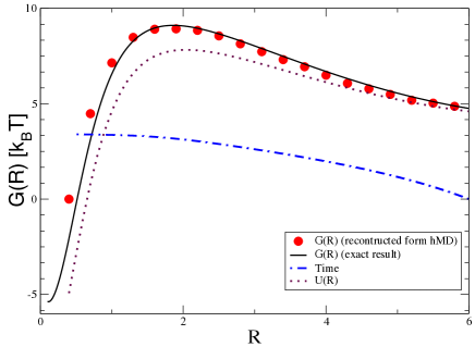
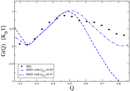
The time evolution for the fraction of native contacts $Q$ (which is a commonly adopted reaction coordinate for protein folding) over a long Langevin trajectory is shown in Fig. 5. The curve shown in the upper panel is compatible with a two-state system, separated by a single low free-energy barrier. This fact is confirmed by the points shown in Fig. 4, which represent the potential of mean-force for this system as a function of $Q$ obtained from a frequency histogram of the same trajectory. The lower panel of Fig. 5 shows the evolution of the fraction of native contacts along a typical folding event. The average transition path time for folding reactions was found to be $\tau^{MD}_{TPT}=(0.50\pm 0.05)$ ns.

Let us now discuss the calculation of the potential of mean-force using the hMD algorithm. We performed 800 independent short hMD simulations with an hindering coefficient of $\xi=3$, starting from the fully stretched configuration. The trajectories were biased using a CC which counts the number of native contacts:

$$z=1-\frac{1}{z_{n}}\sum_{i<j}(C(x_{i},x_{j})-G_{ij})^{2},$$ (20)

where $z_{n}=\sum_{i<j}G_{i,j}$,

$$C(x_{i},x_{j})=\frac{1-(|x_{i}-x_{j}|)/r_{0})^{6}}{1-(|x_{i}-x_{j}|/r_{0})^{10}},$$ (21)

and $r_{0}=0.7$ nm. This biasing biasing CC was shown to be very efficient in guiding ratchet-and-pawl protein folding simulations ratchetMD ; DRPpnas .

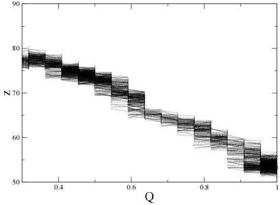
In order to ease the physical interpretation of the results, we choose to reconstruct the free-energy surface as a function of the fraction of native contacts $Q$, rather than of the biasing variable $z$. We recall that, in order for the same hMD procedure to be transferable from the biasing coordinate to a reaction coordinate, the two variables should be directly proportional. Unfortunately, in general, this is not the case for $Q$ and $z$, as it is evident from the fact that the biasing variable can be increased not only by forming a native contact, but also by breaking a non-native contact. However figure 6 shows that, while the linear correlation between $z$ is $Q$ can be violated in general, it is actually respected to good accuracy along the hMD folding trajectories, hence allowing the application of Eq.s (6) and (7).

Figure 6: (Color online) Correlation between the ratchet variable $z$ and the fraction of native contacts $Q$ along the hMD trajectories used to reconstruct the free-energy surface.

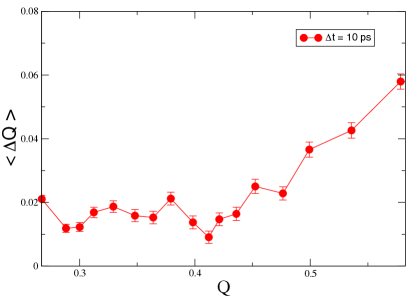
From the ensemble of hMD trajectories we have evaluated the average and average-square displacements of the fraction of native contacts, $\langle\Delta Q(Q)\rangle$ and $\langle\Delta Q^{2}(Q)\rangle$. The most straightforward way to reconstruct $G(Q)$ and compute $\gamma_{Q}$ from these averages consists in using Eq. (7) to fit $\gamma_{Q}$ (hence compute the diffusion coefficient $D_{Q}=k_{B}T/\gamma_{Q}$ ), and then insert this value into Eq. (6) to extract $G^{\prime}(Q)$. However, in the case of the present system, we have observed that higher-order corrections to Eq. (7) introduce some modulation in $\langle\Delta Q^{2}(Q)\rangle$, which spoil the accuracy of an estimate of $\gamma_{Q}$ based on a constant fit. We have therefore developed a different protocol to evaluate $G(Q)$ from the hMD averages, inspired by observation that the hindering of the dynamics should be suppressed once the system crosses the TS. Indeed, beyond this point, the molecule is rapidly and spontaneously relaxing to the product state, hence we expect that the mean displacement $\langle\Delta Q(Q)\rangle$ evaluated in hMD trajectories should undergo a rapid increase at the TS.

Fig. 7 shows the calculated $\langle\Delta Q(Q)\rangle$ —evaluated over the time interval $\Delta t=10$ ps—, which displays a steep increase in the region $0.47\lesssim Q\lesssim 0.50$, which represents our estimate for the location of the TS. Using $G^{\prime}(Q_{TS})=0$, Eq. (6) leads to the estimate $\gamma_{Q}=(3200\pm 1000)$ amu ps^-1. Once this parameter has been fixed, Eq. (6) yields $G^{\prime}(Q)$ in all other points.

Figure 7: (Color online) Average displacement of the fraction of native contacts $\langle\Delta Q\rangle$ evaluated over a time interval $\Delta t=10$ ps in the hMD simulation, as a function of the fraction of native contact $Q$.

The results for the potential of mean-force are reported in Fig. 4 and show that the hMD algorithm is able to identify the two-state character of the reaction kinetics and gives a free-energy barrier to fold which is in very good agreement with the results of MD simulations. On the other hand, the prediction for the free-energy profile is much less accurate in the region from the TS to the native state. This fact is expected, since in the hMD approach the free-energy is obtained by comparing local fluctuations of the velocity in the presence and absence of the hindering. Clearly, beyond the TS the hindering is suppressed and the method becomes inaccurate. This does not represent a problem, since the unfolding free-energy barrier may in principle be calculated by the same algorithm using a different bias which drives the chain from the native to the denatured state.

Figure 8: (Color online) The time at which each value of the CC is visited, computed from the DRP equation (14) using the calculated $G(Q)$ and $\gamma_{Q}$. The dotted line shows the residence time $dt(Q)$, i.e. the integrand of Eq. (14). The initial condition is represented by the point on the left of the plot.

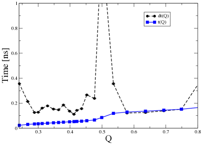
The time at which each value of the CC is visited, computed from the DRP equation (14) using the calculated $G(Q)$ and $\gamma_{Q}$ is shown in Fig. (8). . The dotted line shows the residence time $dt(Q)$, i.e. the integrand of Eq. (14). We note that the residence time is longer in the region around $Q\simeq 0.5$. The same feature is observed in the unbiased Langevin simulations (cfr. the lower panel in Fig.5). The DRP estimate for the total TPT is $\tau_{TPT}\simeq 0.45\pm 0.15$ ns, again in good agreement with the results of the MD simulations, $\tau^{MD}_{TPT}=(0.50\pm 0.05)$ ns. We emphasize that the number of hMD trajectories needed to reconstruct $G(Q)$ and compute $\tau_{TPT}$ is of the same order of those which have been generated in our previous atomistic DRP simulations of protein folding.

V Conclusions

In this work we have introduced an accelerated MD which allows to compute the free-energy profile $G(Q)$ and the diffusion coefficient $D_{Q}$ which describe the stochastic dynamics of a previously determined slow collective variable $Q$. By applying the DRP formalism we have shown that, once $G(Q)$ has been calculated, it is straightforward to obtain an estimate of the TPT, which holds up to logarithmic corrections.

The main advantages of the present method are (i) that the acceleration of the dynamics is not generated by any external force and (ii) that the systematic errors introduced in order to accelerate the overcoming of the free-energy barriers can be analytically computed, hence corrected for.

A few remarks on the limitations of this method are in order. First, we emphasize that it relies on the possibility of identifying a single slow reaction coordinate for the macromolecular system (a list of methods developed to this purpose can be found e.g. in Ref.s RC1 ; RC2 ; RC3 ; RC4 ; RC5 ; RC6 ). If a poorly chosen reaction coordinate is used, the free-energy profile is not expected to capture the correct rate-limiting barrier, and reaction rate calculation will be exponentially inaccurate.

In general, it is not always possible to identify a single slow coarse variable (see e.g. in maze problem maze ). In these cases, our method is expected to miss substantial entropic contributions to the free-energy. Finally, we have found that the free-energy reconstruction is much less accurate in the region connecting the transition state to the product.

All such limitations significant impact on the accuracy of free-energy profile calculations and reaction kinetics. On the other hand, the calculation of the TPT and of the time intervals between consecutive frames in DRP reaction paths are expected to be much more reliable, as the depend only logarithmically on the free-energy.

References

- (1) E.A. Shank, C.Cecconi, J.W. Dill, S. Marqusee and C.Bustamante, Nature 465, 637 (2010).
- (2) W.A. Linke and A. Grützner, Eur. J. Physiol. 456, 101 (2008).
- (3) A. Imparato and L. Peliti, E. Phys. Lett. 69, 643 (2005). A. Imparato, F. Sbrana, and M. Vassalli. E. Phys. Lett. 82, 52006 (2008).
- (4) B. Schuler and W. A. Eaton, Curr. Opin. Struct. Biol. 18, 16 (2008).
- (5) H.S.Chung, K. McHale, J.M. Louis and W.A. Eaton, Science, 335, 981 (2012).
- (6) A. Laio and M. Parrinello, Proc. Natl. Acad. SCI USA 99, 12562 (2002).
- (7) M Chen, M.A. Cuendet and M. E. Tuckerman, J. Chem. Phys. 137 024102 (2010)
- (8) Weinan E, W. Ren, and E. Vanden-Eijnden, Phys. Rev. B 66, 052301 (2002)
- (9) R. Elber, A. Gosh and A. Cardenas, Acc. Chem. Res. 35, 396 (2002).
- (10) P.G. Bolhuis, C. Dellago and D. Chandler, Proc. Natl. Acad. Sci. USA 97, 5877 (2000).
- (11) P. Eastman, N.Gronbech-Jensen, and S. Doniach, J. Chem. Phys. 114, 3823 (2002).
- (12) P. Faccioli, J. Chem. Phys. 133, 164106 (2010).
- (13) Y. Zhao, F.K. Sheong, J. Sun, P. Sander and X. Huang, J. Comput. Chem., doi: 10.1002/jcc.23110 (2012).
- (14) M. E. Johnson and G. Hummer, J. Phys. Chem. B 116, 8573 (2012)
- (15) D. Shirvanyants, F. Ding, D.Tsao, S. Ramachandran and N. V. Dokholyan, J. Phys. Chem. B 116, 8375 (2012).
- (16) D. Moroni, T.S. van Erp, P. G. Bolhuis, Physica A 340, 395 (2004)
- (17) A. K. Faradjian and R. Elber, J. Chem. Phys. 120, 10880 (2004)
- (18) H. Jang and T. B. Woolf, J. Comp. Chem. 27 1136 (2006)
- (19) R. Elber, and D. Shalloway, J. Chem. Phys. 112, 5539 (2000).
- (20) P. Faccioli, M. Sega, F. Pederiva, and H. Orland, Phys. Rev. Lett. 97, 1 (2006).
- (21) M. Sega, P. Faccioli, F. Pederiva, G. Garberoglio, and H. Orland, Phys. Rev. Lett. 99, 1 (2007). S. a Beccara, G. Garberoglio, P. Faccioli and F. Pederiva, J. Chem. Phys. 132 111102 ( 2010).
- (22) S. a Beccara, T. Skrbic, R. Covino and P. Faccioli, Proc. Natl. Acad. Sci. USA 109, 2330 (2012).
- (23) C. Camilloni, R.A. Broglia, and G. Tiana, J. Chem. Phys. 134, 045105 (2011). E. Paci and M. Karplus, J. Mol. Biol. 288 (1999), 441.
- (24) D.E. Shaw et al., Science 330, 341 (2010).
- (25) T. Skrbic, R.Covino, S. a Beccara, C. Micheletti and P. Faccioli, submitted for publication.
- (26) E. Pitard and H. Orland, Europhys. Lett. 41, 467 (1998).
- (27) G. Mazzola, S. a Beccara, P. Faccioli, and H. Orland, J. Chem. Phys. 134, 164109 (2011). P. Faccioli, J. Phys. Chem B112, 13756 (2008).
- (28) P. Faccioli, A. Lonardi and H. Orland, J. Chem. Phys. 133, 045104 (2010).
- (29) N. Go, Annu. Rev. Biophys. Bioeng. 12, 183 (1983).
- (30) K.A. Dill, Biochemistry 24, 1501 (1985).
- (31) W. E, W. Ren, and E. Vanden-Eijnden, Chem. Phys. Lett. 413, 242 (2005).
- (32) B. Peters and B.L. Trout, J. Chem. Phys. 125, 054108 (2006).
- (33) A. Ma, and A. R. Dinner, J. Phys. Chem. B 109, 6769 (2005).
- (34) B. Peters, J. Chem. Phys., 125, 241101 (2006).
- (35) J.D. Chodera, and V.S. Pande, Phys. Rev. Lett., 107, 098102 (2011).
- (36) S. Kirmizialtin, and R. Elber, J. Phys. Chem. A 115, 6137 (2011).
- (37) W. E and E. Vanden-Eijnden, Annu. Rev. Phys. Chem. 61 391 (2010).