Stripe-tetragonal phase transition in the 2D Ising model with dipole interactions: Partition-function zeros approach

Abstract

We have performed multicanonical simulations to study the critical behavior of the two-dimensional Ising model with dipole interactions. This study concerns the thermodynamic phase transitions in the range of the interaction $\delta$ where the phase characterized by striped configurations of width $h=1$ is observed. Controversial results obtained from local update algorithms have been reported for this region, including the claimed existence of a second-order phase transition line that becomes first order above a tricritical point located somewhere between $\delta=0.85$ and 1. Our analysis relies on the complex partition function zeros obtained with high statistics from multicanonical simulations. Finite size scaling relations for the leading partition function zeros yield critical exponents $\nu$ that are clearly consistent with a single second-order phase transition line, thus excluding such tricritical point in that region of the phase diagram. This conclusion is further supported by analysis of the specific heat and susceptibility of the orientational order parameter.

I Introduction

The two-dimensional (2D) Ising model with nearest neighbor ferromagnetic exchange interaction ($J>0$) and dipolar interaction ($g>0$) presents a rich phase diagram because of these competing interactions. This model has been the focus of considerable theoretical interest, and the study of its phase diagram has revealed a variety of unusual magnetic properties. Moreover, at atomic level, it may give some insight into the interactions that form the striped phases observed in a number of ultrathin magnetic films debell_72_2000 ; portmann_422_2003 as a consequence of the reorientation transition of their spins at finite temperatures. The thermodynamic behavior has been investigated by analytical methods and Monte Carlo (MC) simulations, aiming at the determination of its critical behavior as a function of the ratio between the exchange and the dipolar interaction parameters, $\delta=J/g$. The Hamiltonian of this model is written as

$${\cal H}=-\delta\sum_{<i,j>}\sigma_{i}\sigma_{j}+\sum_{i<j}\frac{\sigma_{i}\sigma_{j}}{r_{ij}^{3}}\,.$$ (1)

The variables $\sigma_{i}=\pm 1$ stand for the Ising spins in square lattices $L\times L$ and are supposed to be aligned out of plane. Here, we have adopted the convention cannas_D168_2002 of summing up over all distinct pairs of lattice spins at distances $r_{ij}$ to define the dipolar interaction $g$. The distances $r_{ij}$ are measured in units of lattice.

Analytical methods include some approximations like spin-wave theory and mean-field, kashuba-1993 ; abanov_54_1995 ; macisaac_51_1995 ; grousson-2000 ; biskup_2007 ; rastelli_PRB76_2007 ; giuliani_2006 ; giuliani_2007 ; cannas_75_2007 ; giuliani_2011 but conclusions like the fact that the spontaneous magnetization is zero for all temperatures and that the $T=0$ configurations present patterns classified as regular checkerboards, irregular checkerboards, or stripes of different widths are important. The checkerboard pattern corresponds to the formation of alternate magnetic domains represented by black and white rectangles. Each of these rectangles contain sites with identical spins and are denoted by $<m,n>$, where $m$ and $n$ stand for lattice units rastelli_PRB76_2007 . Regular and irregular checkerboards are defined for $m=n$ and $m\neq n$, respectively. The striped patterns correspond to the formation of magnetic domains displayed in rectangles of size $<m,n>$ but with $n\rightarrow\infty$.

Figure 1: Phase diagram: ($\circ$) data from Ref. rastelli_PRB76_2007 , ($\blacklozenge$) this work. Vertical dotted lines represent the phase boundaries through a sequence of phases characterized by antiferromagnetic (AF) ground state configurations, the $h=1$ and $h=2$ striped phases. The continuous line corresponds to the expected second-order transition except in the narrow $\delta$ range $[0.4152,0.4403]$, and the dashed line $(---)$ refers to a first-order one according to Ref. rastelli_PRB76_2007 and rastelli_73_2006 .

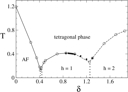
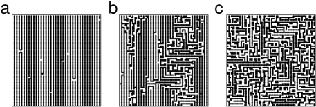
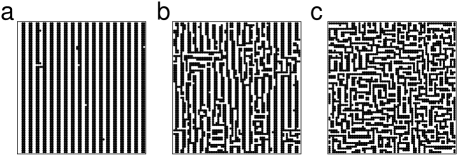
Efforts have been made toward a rigorous theoretical proof for the spontaneous formation of these $T=0$ configurations giuliani_2006 ; giuliani_2007 . The formation of such patterns as a consequence of the long-range character of the dipolar interaction has been confirmed by MC simulations in different regions of the phase diagram $(\delta,T)$. In Fig. 1 we show the phase diagram obtained from MC simulations for the $\delta$ range $[0,1.9]$ where the above described ground-state patterns occur. The particular case $\delta=0$, a pure dipole interaction model, presents a continuous phase transition with critical exponents in agreement with the ones in the universality class of the 2D Ising model rastelli_73_2006 ; macisaac_46_1992 . For $0<\delta<0.4152$, the model presents antiferromagnetic (AF) ground-states characterized by stable regular checkerboard-like spin configurations $<1,1>$. Estimates from the specific heat indicate a continuous thermodynamic phase transition associated with the change from this AF phase to a phase with broken orientational order, the so-called tetragonal phase rastelli_PRB76_2007 . In this phase, the magnetic domains lose their common orientation and try to assume the lattice symmetry. The regular checkerboard configurations change to irregular checkerboard-like configurations $<1,n>$ in the narrow range $0.4152<\delta<0.4403$. In this $\delta$ range, a thermodynamic first-order phase transition seems to take place rastelli_PRB76_2007 . For larger $\delta$ values, the ground state changes to spin configurations characterized by magnetic domains displayed in stripes of alternating spins, whose stripe width $h$ increases with $\delta$ macisaac_51_1995 ; giuliani_2007 . Striped configurations of width $h=1$ and $h=2$ occur for $0.4403<\delta<1.2585$ and $1.2585<\delta<2.1724$, respectively. Figures 2 and 3 contain these magnetic patterns obtained from our simulations for the couplings $\delta=1.20$ and $\delta=1.30$, respectively. In figure 2(a), the low-temperature ($T=0.270$) simulation at $\delta=1.20$ presents stripes of width $h=1$. Our simulations indicate a transition from the striped to the tetragonal phase at $T_{c}=0.311$ (figure 2(b)). The tetragonal phase is depicted in Figure 2(c). Figure 3 presents magnetic patterns from simulations performed at $\delta=1.30$, a region where stripes of width $h=2$ occur.

Figure 2: Spin configurations for $\delta=1.20$ and $L=72$. (a) striped phase: $T=0.270$, $E/N=-0.4638$, $O_{hv}=0.9869$; (b) transition temperature: $T_{c}=0.311$, $E/N=-0.4096$, $O_{hv}=0.5039$; (c) tetragonal phase: $T=0.350$, $E/N=-0.3539$, $O_{hv}=0.0476$.

Figure 3: Spin configurations for $\delta=1.30$ and $L=72$. (a) striped phase: $T=0.290$, $E/N=-0.5058$, $O_{hv}=0.9831$; (b) transition temperature: $T_{c}=0.329$, $E/N=-0.4397$, $O_{hv}=0.5173$; (c) tetragonal phase: $T=0.380$, $E/N=-0.3821$, $O_{hv}=0.0370$.

In addition to the striped and tetragonal phases, a new domain in the phase diagram has been reported for $\delta=2$, the so-called nematic phase in analogy with liquid crystals. In the nematic phase the system still keeps its long-range orientational order but loses the spatial order exponentially. This new domain has been studied by MC simulations, and it has been found between the striped and the tetragonal phases. In this case, we would have two thermodynamic phase transitions: stripe-nematic and nematic-tetragonal transitions. This new phase is located in a region of the $(\delta,T)$ plane that gives origin to a bifurcation of the line that separates the $h=2$ and $h=3$ phases cannas_73_2006 ; rizzi_2010 .

A convincing determination of the thermodynamic phase-transition order is still lacking even for such small $h$ values. In fact, controversial results about the order of the thermodynamic phase transition as a function of $\delta$ have been reported in the literature. In particular, some MC results concerning square lattices for $\delta$ between 0.2 and 2 exhibit a phase diagram with a second-order transition line cannas_D168_2002 ; cannas_68_2003 for the thermodynamic transition between the ordered phases and the tetragonal one. On the other hand, the transition line appears to be first order for a $\delta$ range corresponding to $h\geq 1$ rastelli_PRB76_2007 , with the remark that for $\delta=0.85$ a second-order phase transition takes place with exponents $d\nu=2.0\pm 0.1$, $\alpha=0.09\pm 0.07$, and $\gamma=1.75\pm 0.05$ at the critical temperature $T_{c}=0.41$ rastelli_73_2006 . As usual, $\nu,\alpha$, and $\gamma$ are the correlation length, specific heat, and susceptibility exponents, respectively. For the interaction $\delta=1$, it seems to be first order at $T_{c}=0.40$ rastelli_PRB76_2007 and to present only a weak first-order character at $T_{c}=0.404$ cannas_73_2006 . The above cited results would lead to the existence of two critical lines separated by a tricritical point for $\delta$ somewhere between 0.85 and 1. cannas_75_2007

The controversial results are a consequence of the dipolar term, which produces large autocorrelations in MC time series obtained with local update algorithms cannas_68_2003 ; cannas_78_2008 ; rizzi_2010 . Moreover, simulations have also been hampered because large lattice size simulations are very CPU time consuming due to this term, frustrating any convincing finite size scaling (FSS) analysis. In this paper, we perform extensive multicanonical simulations for determination of the character of the thermodynamic transition from the $h=1$ phase, and to address the existence of a tricritical point. The multicanonical algorithm (MUCA) generates a 1D random walk in the energy space, diminishing the problem of overcoming free energy barriers. We carry out a comprehensive analysis of the character of the phase transition for values of $\delta$ from 0.85 up to 1.30 by means of the complex partition function zeros fisher-1965 ; itzykson . Partition function zeros analysis in the complex temperature plane has been successfully applied to spin models salvador1987 ; alvesB1990 ; alvesB1991 , lattice gauge theories alvesPRL1990 ; alvesB1992 , and protein models alvesPRL2000 ; ferrite2002 . This procedure has allowed us to explore critical aspects by means of FSS relations for the first complex zero, leading to a precise characterization of the phase transition line. The conclusions based on the partition function zeros are further supported by analysis of the specific heat and susceptibility of the orientational order parameter. Analysis of these thermodynamic quantities allows us to calculate the critical exponents $\alpha/\nu$ and $\gamma/\nu$. It is well known that the renormalization-group fixed point picture for $d$-dimensional systems in the $L^{d}$ block geometry characterizes a first-order phase transition by the particular value of the critical exponent $d\nu=1$ fisher-nu ; decker_1988 . This, in turn, gives $\alpha=1$ and $\gamma=1$ for a first-order phase transition, which produce the expected dependence of the thermodynamic quantities on the volume $L^{d}$ and has been supported in a number of Monte Carlo studies fukugita ; alvesB1991 .

Our results rely on data collected from lattice sizes up to $L=72$. We report precise estimates for the infinite volume critical temperatures and critical exponents $\nu$, $\alpha/\nu$, and $\gamma/\nu$ for values of $\delta$ from 0.85 up to 1.20. We have included the interaction $\delta=1.30$ in the $h=2$ phase for comparative purposes. In Sec. II, we briefly review the main aspects of MUCA, and the protocol devised for updating of the multicanonical parameters. In Sec. III, results from FSS relations for the first complex zero, specific heat, and susceptibility are compiled, to produce the estimates for the critical exponents. The final Sec. IV presents a summary and our main conclusions.

II Multicanonical simulations

The multicanonical algorithm berg-fields ; berg-2003 , like other generalized algorithms okamoto-2001 , significantly improves the sampling of configurations. This algorithm assigns a weight $w_{mu}(E)\simeq 1/n(E)$, where $n(E)$ is the density of states and $E={\cal H}(\{\sigma_{i}\})$ is the energy of a state given by the spin configuration $\{\sigma_{i}\}$, with $i=1,...,L^{2}$, as defined in Eq. (1). Therefore, the multicanonical method is expected to produce flat energy histograms $H_{mu}(E)\propto n(E)w_{mu}(E)$ under the following probability condition

$$p(E\rightarrow E^{\prime})=\min\left[1,\frac{w_{mu}(E^{\prime})}{w_{mu}(E)}\right]$$ (2)

for sufficiently long simulation times.

The multicanonical weight $w_{mu}(E)$ is a priori unknown. A numerical estimate of $w_{mu}(E)$ is usually obtained by considering the Boltzmann entropy $S(E)=\ln n(E)$ ($k_{B}=1$), and the following parameterization for the entropy $S(E)=b(E)E-a(E)$, where $a(E)$ and $b(E)$ are called multicanonical parameters. Hence, the multicanonical weight is given by $w_{mu}(E)={\rm exp}[-b(E)E+a(E)]$, with the parameter $a(E)$ related to a multicanonical free energy and $b(E)$ related to the inverse of the microcanonical temperature.

The implementation of MUCA requires energy discretization. An integer label $m$ is introduced to facilitate our histogramming of energy data. This label defines energy bins of size $\varepsilon$, $E_{m}=E_{0}+m\varepsilon$, with $m=0,\cdots,M$. All the energies in the interval $[E_{m},E_{m+1}[$ are in the $m$th energy bin and contribute to the histogram $H_{mu}(E_{m})$. The constant $E_{0}$ is defined as a reference energy just below the ground-state energy. We have verified that $\varepsilon=1$ is a convenient discretization.

The parameters $a(E)$ and $b(E)$ are estimated from $N_{r}$ recursion steps. Each step updates the multicanonical parameters through the following equations berg-fields ,

$$a^{n}(E_{m-1}) = a^{n}(E_{m})+[b^{n}(E_{m-1})-b^{n}(E_{m})]E_{m}~{},$$

$$b^{n}(E_{m}) = b^{n-1}(E_{m})+[\ln\hat{H}^{n-1}_{mu}(E_{m+1})-\ln\hat{H}^{n-1}_{mu}(E_{m})]/\varepsilon~{},$$ (3)

where $n$ ($n=1,\cdots,N_{r}$) labels the recursion steps and $N_{r}$ amounts to how long this update procedure is enforced in order to obtain reliable estimates for $w_{mu}(E)$. The choice $\hat{H}^{n}_{mu}(E_{m})=\max[h_{0},H^{n}_{mu}(E_{m})]$, with $0<h_{0}<1$ for all discretized energies, is a technical choice to avoid $H(E_{m})=0$ berg-fields . It is convenient to compute the above recurrence relations with the initial conditions $a^{0}(E_{m})=0$ and small values for $b^{0}(E_{m})$ if the simulation uses a hot-start initialization. The $n$th recursion step needs the calculation of $H_{mu}(E_{m})$ from the previous weight $\{a^{n-1},b^{n-1}\}$, obtained with $n_{s}$ MC sweeps. Usually, the number $N_{r}$ is defined a posteriori when the multicanonical parameters present some convergence.

To determine the multicanonical parameters, we have devised the following protocol. Each recursion step is implemented after collection of $H_{mu}$ data by sampling configurations between two extremal energies $E^{*}_{-}$ and $E^{*}_{+}$, with $E^{*}_{-}<E^{*}_{+}$. A round trip is defined as the number of sweeps necessary to go from configurations with the lowest reference energy $E^{*}_{-}$ to the ones with a fixed high energy $E^{*}_{+}$ and back. A round-trip walk may also start at any energy between $E^{*}_{-}$ and $E^{*}_{+}$. The multicanonical update procedure Eq. (3) is performed with a variable number of MC sweeps necessary for the attainment of three of such round trips. This number of round trips is chosen to ensure samplings across the energy landscape in a reasonable simulation time. To avoid too long simulation time to achieve the next $(n+1)$th multicanonical recursion, a fixed number of sweeps $n_{s}(n)$ is set as the limiting number of MC updates. Thus, new multicanonical parameters are obtained as soon as one of the following conditions is observed: a) three round trips or b) a number of MC sweeps greater than three times the average number of MC sweeps counted in the previous multicanonical simulations,

$$n_{s}(n)=\frac{3}{n-1}\sum_{i=1}^{n-1}n_{s}(i)\,.$$ (4)

After each multicanonical update, $E^{*}_{-}$ is replaced with the minimum energy among the sampled energies in the previous simulation. This establishes a new (and larger) energy interval where new round trips must occur. This protocol helps us to keep a reasonable number of tunneling events even for large lattice sizes at the price of longer CPU times. A further improvement of the multicanonical weight $w_{mu}^{N_{r}}$ is achieved with an extra MUCA update, which consists of $n_{MC}$ MC sweeps necessary for the performance of 20 round trips. Table I lists only the number of sweeps $n_{MC}$ as a function of the lattice size $L$ for different interactions $\delta$ that are necessary for the accomplishment of this final update. With this final estimate of the multicanonical weight $w_{mu}(E)$, we proceed to data production. Our data production amounts to 16 independent energy time series, each one produced with $n_{MC}$ sweeps. Thus, the data analysis for the smallest lattice size $L=12$ and $\delta=0.89$ relied on $\simeq 1.8\times 10^{5}$ measurements, while in the case of the largest lattice size $L=72$ and $\delta=1.30$ it amounted to $\simeq 1.62\times 10^{8}$ measurements. We can anticipate that the large number of measurements for $\delta=1.30$, compared with the smaller $\delta$ values, is related to the effort of overcoming the free energy barrier as a consequence of a first-order phase transition at this interaction.

We have carried out simulations with periodic boundary conditions to minimize border effects. Thus, all distances $r_{ij}$ must include sites in the infinitely replicated simulation box in both directions. This boundary condition adds an infinite sum over all images of the simulation box because of the dipole term in the Hamiltonian. The infinite sum was computed by means of the Ewald summation technique. This technique splits the infinite sum over all images of the system into two quickly converging sums, namely the direct sum, which is evaluated in the real space, and the reciprocal sum, carried out in the reciprocal space, as well as a self-interaction correction term CompPhysComm.95.1996 ; JChemPhys.106.1997 . We set the Ewald parameter $\alpha$ to 3.5 in all the simulations. This parameter determines the rate of convergence between the two sums.

An important consequence of MUCA data production is the estimation of canonical averages of thermodynamic quantities $A$ over a wide range of temperatures $T=1/\beta$ by using the reweighting technique ferrenberg_61_1988

$$\overline{A(\beta)}=\frac{\sum_{k}\,A_{k}\,[w_{mu}^{N_{r}}(E_{k})]^{-1}\exp{(-\beta E_{k})}}{\sum_{k}[w_{mu}^{N_{r}}(E_{k})]^{-1}\exp{(-\beta E_{k}})}\,.$$ (5)

This contrasts with the Metropolis algorithm, where the reweighting is restricted to a very narrow temperature range around the fixed MC simulation temperature. After reliable estimates for the MUCA weight, one can evaluate the density of states

$$n(E)=H_{mu}(E)w^{-1}_{mu}(E),$$ (6)

from which one can construct the partition function

$$Z(\beta)=\sum_{E}n(E)u^{E},$$ (7)

where $u=e^{-\beta}$. The complex solutions in $u$, $\{{\rm Re}(u),{\rm Im}(u)\}$, describe the critical behavior of the system. These solutions correspond to the so-called Fisher zeros fisher-1965 ; itzykson .

III Results

III.1 Partition function zeros

Let us consider the complex zeros of Eq. (7) ordered according to their increasing imaginary part. For a sufficiently large lattice size $L$, the leading partition function zero $u_{1}^{0}(L)$ can be used to obtain the critical exponent $\nu$ through the FSS relation itzykson ,

$$u_{1}^{0}(L)=u_{c}+AL^{-1/\nu}[1+O(L^{y})]~{},~{}~{}~{}~{}~{}~{}y<0.$$ (8)

This relation shows that the distance from the closest zero $u_{1}^{0}$ to the infinite lattice critical point $u_{c}=e^{-\beta_{c}}$ on Re($u$) scales with the lattice size. If we disconsider finite size corrections, the exponent $\nu$ can be obtained from the linear regression

$$-\,{\rm ln}\,|u_{1}^{0}(L)-u_{c}|=\frac{1}{\nu}\,{\rm ln}(L)+a~{}.$$ (9)

Since the exact critical temperature is unknown, and because the real part of $u$ presents weaker dependence on $L$ as compared to the imaginary part of $u$, it is usual to replace $|u_{1}^{0}-u_{c}|$ with its imaginary part, so as to avoid a multiparameter fit.

With the discretization $\varepsilon$, Eq. (7) becomes a polynomial in $u$ and it can be solved with MATHEMATICA for $L\leq 32$. Larger lattices present huge numbers for the density of states, which makes the scan method in the complex temperature plane the only way of obtaining complex zeros alvesC1997 . The leading complex zeros are presented in Tables II, III, and IV as a function of $L$ for different $\delta$ values.

Now, considering the real part of those zeros, ${\rm Re}\,[\beta_{1}^{0}(L)]=-1/2\,{\rm ln}\{[{\rm Re}\,u_{1}^{0}(L)]^{2}\,+[{\rm Im}\,u_{1}^{0}(L)]^{2}\}$, one can estimate the critical temperatures through the following FSS fit fukugita :

$${\rm Re}\,[\beta_{1}^{0}(L)]=\beta_{c}^{0}+bL^{-1/\nu}~{}.$$ (10)

This fit yields the critical temperatures $T_{c}^{0}$ displayed in Table V, where we have included the exponents $d\nu$.

Figure 4: Finite-size scaling fits of the leading complex zeros for some $\delta$ couplings.

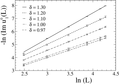
The quality of the linear fits can be stated in terms of the goodness-of-fit of the model recipes . The goodness-of-fit $Q$, $(0\leq Q\leq 1)$ is related to $\chi^{2}$ and, as a general rule, if $Q$ is larger than 0.1, then the fit is believable. The linear fits for evaluation of $\nu$ present $Q$ as large as 0.98 for $\delta\leq 1.10$, $Q=0.70$ for $\delta=1.20$, and a very small $Q$ value $\simeq 10^{-10}$ for $\delta=1.30$. Figure 4 illustrates our linear fits for $\delta\geq 0.97$. The data fit nicely, confirming the linear dependence on ${\rm ln}(L)$. However, the very small $Q$ value for $\delta=1.30$ seems to be a consequence of high statistical precision for these zeros (see Fig. 4), which reveals the presence of some systematic bias. It is known that corrections to FSS relations give a better fit for first-order phase transitions fukugita . However, this would require larger lattice sizes for the attainment of reliable estimates from a multiparameter fit. The asymptotic behavior of $T_{1}^{0}(L)$ is determined with high $Q$ values for all $\delta$ interactions. Data collected in the third column of Table V shows a consistent trend toward $d\nu=1$ as we move on the critical line in the direction of higher $\delta$. The value $d\nu=1$ is only reached for the interaction in the $h=2$ phase. Thus, these results clearly exclude first-order phase transitions from the $h=1$ phase.

Results for $T_{c}^{0}$ are depicted in Fig. 1 with the symbol ($\blacklozenge$). In this figure we also show the values obtained from Ref. rastelli_PRB76_2007 and, in particular, we note that the values for $\delta=0.85$ and 1.3 are surprisingly good as compared to $T_{c}^{0}$, since they are obtained from a single lattice size $L=48$.

III.2 Specific heat and susceptibility

To further characterize the order of the phase transitions, we have studied the specific heat,

$$C_{v}(T)\ =\ \frac{1}{T^{2}N}(\langle E^{2}\rangle-\langle E\rangle^{2})\,,$$ (11)

and the susceptibility

$$\chi(O_{hv})=N\left(\langle O_{hv}^{2}\rangle-\langle O_{hv}\rangle^{2}\right),$$ (12)

associated with the orientational order parameter ibooth_75_1995 ,

$$O_{hv}=\left|\frac{n_{v}-n_{h}}{n_{v}+n_{h}}\right|,$$ (13)

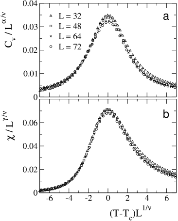
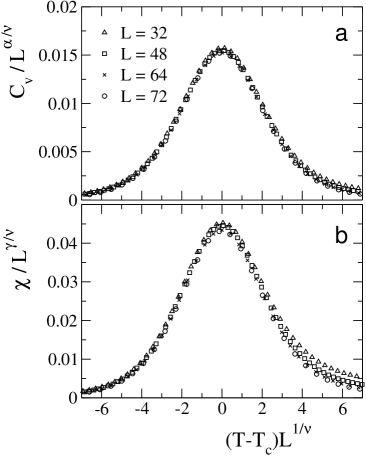
over a (continuous) range of temperatures by reweighting MC data according to Eq. (5). The quantities $n_{h}$ and $n_{v}$ are the number of horizontal and vertical bonds of the nearest neighbor antiparallel spins, respectively. This order parameter is $+1$ in the striped ground state, and it vanishes at high temperatures where orientational symmetry of the striped domain is broken. A very common way of obtaining the critical exponents is through the FSS relations for the maximum of the specific heat

$$C_{v}|_{\rm max}(T_{c}(L),L)\propto L^{\alpha/\nu}\,$$ (14)

and for the maximum of the susceptibility,

$$\chi_{\rm max}(T_{c}(L),L)\propto L^{\gamma/\nu}\,,$$ (15)

where $T_{c}(L)$ is the finite size critical point. Again, an FSS relation like Eq. (10) is applied to the temperatures $T_{c}(L)$, where the maxima of $C_{v}(T,L)$ and $\chi(T,L)$ occur, to yield the infinite volume critical temperature $T_{c}^{C_{v}}$ and $T_{c}^{\chi}$, respectively. Table V summarizes these temperatures and the critical exponents for $C_{v}$ and $\chi$. The temperatures $T_{c}^{C_{v}}$ and $T_{c}^{\chi}$ are then evaluated with $\nu$ obtained from the hyperscaling relation $\alpha=2-d\nu$, with data displayed in the 5th column of table V. The goodness-of-fit of the linear fit for $C_{v}$ is about 0.5 for $\delta\leq 1.20$. Again, it decreases to a very small value $Q\simeq 10^{-5}$ for $\delta=1.30$. The linear fit of $\chi$ presents $Q\simeq 0.8$ for $\delta\leq 1.20$ and also decreases to $10^{-5}$ for $\delta=1.30$.

The critical exponents $\alpha/\nu$ in the 5th column (Table V) clearly exclude any possibility of a first-order phase transition from the $h=1$ phase, while it strongly indicates this possibility at $\delta=1.30$. The statistical error bar exclude the value $\alpha/\nu=2$ at $\delta=1.30$, but the small $Q$ value may indicate the presence of systematic bias. The results from the susceptibility are less prompt to make satisfactory claims about the order of the phase transition only at $\delta=1.2$ and $1.3$. Again, those results may be due to the missed corrections to the FSS relation, as expected at first-order phase transitions. Figures 5 and 6 display the FSS plots for $C_{v}(T_{c}(L),L))$ and $\chi(T_{c}(L),L))$ for $\delta=1.20$ and $1.30$, respectively. These figures have helped us observe how satisfactory the FSS are.

Figure 5: Finite-size scaling plots for the (a) specific heat and (b) susceptibility as a function of the temperature for $\delta=1.20$.

Figure 6: Finite-size scaling plots for the (a) specific heat and (b) susceptibility as a function of the temperature for $\delta=1.30$.

IV Summary and Conclusions

We have performed analysis of the complex partition function zeros from multicanonical simulations. The sampling with this algorithm is known to be efficient when it comes overcoming the free-energy barrier problem in simulations of complex systems as compared to the usual local update algorithms. MUCA is based on a non-Boltzmann weight factor and performs a free one-dimensional random walk in the energy space. A protocol has been devised for the determination of the multicanonical weight factor by ensuring that enough measurements in the energy space are obtained. Moreover, by keeping such control over the number of round trips between the low and high-energy configurations, we were able to determine the number of sweeps that is necessary for exploration of the energy space even for large lattice sizes.

By using FSS relations involving the partition-function zeros obtained with high statistics, precise estimates for the infinite-volume critical temperatures and critical exponents $\nu$ were found for interactions $\delta$ corresponding to the $h=1$ phase. We also included an interaction ($\delta=1.30$) that produces stripes of width $h=2$ for comparative purposes. Analysis of the specific heat and susceptibility of the order-disordered parameter $O_{hv}$ gives further support for a second-order transition critical line from the $h=1$ phase. Infinite volume critical temperatures obtained from $u_{1}^{0}$, maximum of $C_{v}$ and $\chi$, are in full agreement, which help us draw a reliable part of the phase diagram $(\delta,T)$. In conclusion, the study conducted with many $\delta$ interactions strongly indicates the existence of a second-order critical line between the high-temperature tetragonal phase and the low-temperature ordered phase characterized by $h=1$. The first-order character is found in our study only for the interaction $\delta=1.30$. This suggests that the second-order critical line ends at $\delta=1.2585$, and that it becomes first-order beyond this point. We assume that both transition lines are separated by a tricritical point at $\delta=1.2585$, because this point produces a line separating the $h=1$ and $h=2$ phases, and it bifurcates for generation of the tetragonal phase. The precise temperature where this bifurcation happens has not been evaluated in the literature to the best of our knowledge.

$L$$\backslash$$\delta$	0.85	0.89	0.91	0.93	0.95	0.97	1.00	1.10	1.20	1.30
$12$	15 018	11 632	12 032	14 026	10 186	16 893	12 279	24 216	51 171	73 362
$20$	65 278	47 290	52 098	46 969	50 127	78 380	63 333	91 158	226 934	269 598
$32$	181 069	188 620	149 412	105 008	158 214	213 036	179 126	236 436	959 554	1 354 207
$48$	401 195	483 287	380 451	645 854	503 469	484 012	582 030	879 740	2 285 886	3 256 588
$64$	1 028 097	824 022	938 475	751 156	1 104 830	1 300 445	1 296 208	2 281 061	5 579 023	8 159 701
$72$	1 283 737	1 345 861	1 421 650	1 332 818	1 709 722	1 590 101	1 697 157	1 975 543	5 682 748	10 171 715

Table 1: Number of MC sweeps $n_{MC}$ as a function of the lattice size $L$ for different interactions $\delta$. These numbers correspond to 20 round trips observed in the final MUCA update.

	$\delta=0.89$		$\delta=0.91$		$\delta=0.93$
$L$	Re$(u_{1}^{0})$	Im$(u_{1}^{0})$	Re$(u_{1}^{0})$	Im$(u_{1}^{0})$	Re$(u_{1}^{0})$	Im$(u_{1}^{0})$
12	0.0913(37)	0.0401(28)	0.0923(36)	0.0381(29)	0.0907(34)	0.0377(21)
20	0.0911(22)	0.0222(14)	0.0909(24)	0.02117(95)	0.0899(14)	0.0205(13)
32	0.0908(12)	0.01330(55)	0.08967(96)	0.01300(90)	0.0886(11)	0.01237(62)
48	0.09035(67)	0.00842(57)	0.08869(99)	0.00807(51)	0.08776(49)	0.00770(50)
64	0.08932(99)	0.00615(39)	0.08864(64)	0.00598(32)	0.08729(54)	0.00568(39)
72	0.08970(60)	0.00556(39)	0.08857(85)	0.00522(41)	0.08711(64)	0.00502(31)

Table 2: Complex partition function zeros for $\delta=0.89,0.91$, and $0.93$.

	$\delta=0.95$		$\delta=0.97$		$\delta=1.00$
$L$	Re$(u_{1}^{0})$	Im$(u_{1}^{0})$	Re$(u_{1}^{0})$	Im$(u_{1}^{0})$	Re$(u_{1}^{0})$	Im$(u_{1}^{0})$
12	0.0895(31)	0.0358(25)	0.0871(21)	0.0339(16)	0.0844(18)	0.0312(16)
20	0.0886(14)	0.0194(10)	0.0858(11)	0.01841(71)	0.08298(86)	0.01637(41)
32	0.08708(82)	0.01157(76)	0.08497(55)	0.01053(47)	0.08162(62)	0.00916(42)
48	0.08634(51)	0.00728(34)	0.08446(42)	0.00677(41)	0.08124(43)	0.00577(23)
64	0.08580(27)	0.00513(17)	0.08408(28)	0.00479(28)	0.08096(17)	0.00406(25)
72	0.08583(31)	0.00460(25)	0.08391(26)	0.00408(21)	0.08068(15)	0.00353(14)

Table 3: Complex partition function zeros for $\delta=0.95,0.97$, and $1.00$.

	$\delta=1.10$		$\delta=1.20$		$\delta=1.30$
$L$	Re$(u_{1}^{0})$	Im$(u_{1}^{0})$	Re$(u_{1}^{0})$	Im$(u_{1}^{0})$	Re$(u_{1}^{0})$	Im$(u_{1}^{0})$
12	0.0666(14)	0.02223(87)	0.0365(14)	0.01504(51)	0.0515(10)	0.01329(29)
20	0.06579(63)	0.01049(34)	0.03968(82)	0.00687(35)	0.05091(45)	0.004203(34)
32	0.06524(48)	0.00544(21)	0.04006(22)	0.00326(17)	0.04876(14)	0.001745(15)
48	0.06504(21)	0.00312(12)	0.040060(91)	0.001584(91)	0.048100(66)	0.0007782(50)
64	0.06488(10)	0.002070(83)	0.039935(59)	0.000974(49)	0.047899(44)	0.0004346(18)
72	0.06476(11)	0.0017227(77)	0.039934(39)	0.000800(47)	0.047868(29)	0.0003433(11)

Table 4: Complex partition function zeros for $\delta=1.10,1.20$, and $1.30$.

$~{}~{}\delta$	$T_{c}^{0}$	$d\nu$	$T_{c}^{C_{v}}$	$\alpha/\nu$	$T_{c}^{\chi}$	$~{}~{}~{}~{}\gamma/\nu$
$0.85$	0.41189(53)	1.837(76)	0.41240(48)	0.344(16)	0.41200(51)	1.519(19)
$0.89$	0.41168(53)	1.807(70)	0.41104(62)	0.364(20)	0.41100(48)	1.531(27)
$0.91$	0.40887(50)	1.817(68)	0.40992(16)	0.375(19)	0.40964(17)	1.538(22)
$0.93$	0.40681(19)	1.779(61)	0.40685(46)	0.399(20)	0.40682(45)	1.561(24)
$0.95$	0.40435(17)	1.741(53)	0.40475(12)	0.424(20)	0.40475(18)	1.552(24)
$0.97$	0.40108(40)	1.706(46)	0.40124(45)	0.461(19)	0.40130(31)	1.575(20)
$1.00$	0.39499(37)	1.659(37)	0.39521(33)	0.522(17)	0.39527(29)	1.590(23)
$1.10$	0.36429(29)	1.415(25)	0.36441(19)	0.888(21)	0.36456(15)	1.736(21)
$1.20$	0.31102(32)	1.223(21)	0.31126(65)	1.496(28)	0.31073(40)	1.987(29)
$1.30$	0.32929(72)	1.0093(28)	0.32892(15)	2.0183(66)	0.32885(14)	2.3193(82)

Table 5: Critical temperatures and critical exponents from complex partition function zeros, specific heat $C_{v}$, and susceptibility $\chi(O_{hv})$.

References

- (1) K. De’Bell, A. B. MacIsaac, and J. P. Whitehead, Rev. Mod. Phys. 72, 225 (2000).
- (2) O. Portmann, A. Vaterlaus, and D. Pescia, Nature 422, 701 (2003); Phys. Rev. Lett. 96, 047212 (2006).
- (3) P. M. Gleiser, F. A. Tamarit, and S. A. Cannas, Physica D 168-169, 73 (2002).
- (4) A. B. Kashuba and V. L. Pokrovsky, Phys. Rev. B 48, 10335 (1993).
- (5) M. Grousson, G. Tarjus, and P. Viot, Phys. Rev. E 62, 7781 (2000).
- (6) A. Abanov, V. Kalatsky, V. L. Pokrovsky, and W. M. Saslow, Phys. Rev. B 51, (1995) 1023.
- (7) S. A. Pighín and S. A. Cannas, Phys. Rev. B 75, 224433 (2007).
- (8) A. Giuliani, J. L. Lebowitz, and E. H. Lieb, Phys. Rev. B 74, 064420 (2006).
- (9) A. Giuliani, J. L. Lebowitz, and E. H. Lieb, Phys. Rev. B 76, 184426 (2007).
- (10) A. Giuliani, J. L. Lebowitz, and E. H. Lieb, Phys. Rev. B 84, 064205 (2011).
- (11) M. Biskup, L. Chayes, and S. A. Kivelson, Commun. Math. Phys. 274, 217 (2007).
- (12) E. Rastelli, S. Regina, and A. Tassi, Phys. Rev. B 76, 054438 (2007).
- (13) A. B. MacIsaac, J. P. Whitehead, M.C. Robinson, and K. De’Bell, Phys. Rev. B 51, 16033 (1995).
- (14) A. B. MacIsaac, J. P. Whitehead, K. De’Bell, and K. S. Narayanan, Phys. Rev. B 46, 6387 (1992).
- (15) E. Rastelli, S. Regina, and A. Tassi, Phys. Rev. B 73, 144418 (2006).
- (16) S. A. Cannas, M. F. Michelon, D. A. Stariolo, and F. A. Tamarit, Phys. Rev. B 73, 184425 (2006).
- (17) L. G. Rizzi and N. A. Alves, Physica B 405, 1571 (2010).
- (18) P. M. Gleiser, F. A. Tamarit, S. A. Cannas, and M. A. Montemurro, Phys. Rev. B 68, 134401 (2003).
- (19) S. A. Cannas, M. F. Michelon, D. A. Stariolo, and F. A. Tamarit, Phys. Rev. E 78, 051602 (2008).
- (20) M. E. Fisher, in Lectures in Theoretical Physics, University of Colorado Press, Boulder, 1965, Vol. 7c, p. 1.
- (21) C. Itzykson, R. B. Pearson, and J. B. Zuber, Nucl. Phys. B 220 [FS8], 415 (1983).
- (22) G. Bhanot, R. Salvador, S. Black, P. Carter, and R. Toral, Phys. Rev. Lett. 59, 803 (1987).
- (23) N. A. Alves, B. A. Berg, and R. Villanova, Phys. Rev. B 41, 383 (1990).
- (24) N. A. Alves, B. A. Berg, and R. Villanova, Phys. Rev. B 43, 5846 (1991).
- (25) N. A. Alves, B. A. Berg, and S. Sanielevici, Phys. Rev. Lett. 64, 3107 (1990).
- (26) N. A. Alves, B. A. Berg, and S. Sanielevici, Nucl. Phys. B 376, 218 (1992).
- (27) N. A. Alves and U. H. E. Hansmann, Phys. Rev. Lett. 84, 1836 (2000).
- (28) N. A. Alves, J. P. N. Ferrite, and U. H. E. Hansmann, Phys. Rev. E 65, 036110 (2002).
- (29) M. E. Fisher and A. N. Berker, Phys. Rev. B 26, 2507 (1982).
- (30) K. Decker, A. Hasenfratz, and P. Hasenfratz, Nucl. Phys. B 295 [FS21], 21 (1988).
- (31) M. Fukugita, H. Mino, M. Okawa, and A. Ukawa, J. Stat. Phys. 59, 1397 (1990), and references given therein.
- (32) B. A. Berg, in Monte Carlo Methods, Fields Institute Communications Vol. 26, edited by N. Madras (American Mathematical Society, Providence, RI, 2000), p. 1.
- (33) B. A. Berg, Comput. Phys. Commun. 153, 397 (2003).
- (34) A. Mitsutake, Y. Sugita, and Y. Okamoto, Biopolymers 60, 96 (2001).
- (35) A. Y. Toukmaji and J. A. Board Jr., Comput. Phys. Commun. 95, 73 (1996).
- (36) G. T. Gao, X. C. Zeng, and W. Wang, J. Chem. Phys. 106, 3311 (1996).
- (37) A. M. Ferrenberg and R. H. Swendsen, Phys. Rev. Lett. 61, 2635 (1988); 63, 1195 (1989).
- (38) N. A. Alves, J. R. D. Felicio, and U. H. E. Hansmann, Int. J. Mod. Phys. C 8, 1063 (1997).
- (39) W. Press et al., Numerical Recipes, Cambridge University Press, London, 1986.
- (40) I. Booth, A. B. MacIsaac, J. P. Whitehead, and K. De’Bell, Phys. Rev. Lett. 75, 950 (1995).