Distributed Maximum Likelihood for Simultaneous Self-localization and Tracking in Sensor Networks

Abstract

We show that the sensor self-localization problem can be cast as a static parameter estimation problem for Hidden Markov Models and we implement fully decentralized versions of the Recursive Maximum Likelihood and on-line Expectation-Maximization algorithms to localize the sensor network simultaneously with target tracking. For linear Gaussian models, our algorithms can be implemented exactly using a distributed version of the Kalman filter and a novel message passing algorithm. The latter allows each node to compute the local derivatives of the likelihood or the sufficient statistics needed for Expectation-Maximization. In the non-linear case, a solution based on local linearization in the spirit of the Extended Kalman Filter is proposed. In numerical examples we demonstrate that the developed algorithms are able to learn the localization parameters.

Collaborative tracking, sensor localization, target tracking, maximum likelihood, sensor networks

1 Introduction

This paper is concerned with sensor networks that are deployed to perform target tracking. A network is comprised of synchronous sensor-trackers where each node in the network has the processing ability to perform the computations needed for target tracking. A moving target will be simultaneously observed by more than one sensor. If the target is within the field-of-view of a sensor, then that sensor will collect measurements of the target. Traditionally in tracking a centralized architecture is used whereby all the sensors transmit their measurements to a central fusion node, which then combines them and computes the estimate of the target’s trajectory. However, here we are interested in performing collaborative tracking, but without the need for a central fusion node. Loosely speaking, we are interested in developing distributed tracking algorithms for networks whose nodes collaborate by exchanging appropriate messages between neighboring nodes to achieve the same effect as they would by communicating with a central fusion node.

A necessary condition for distributed collaborative tracking is that each node is able to accurately determine the position of its neighboring nodes in its local frame of reference. (More details in Section 2.) This is essentially an instance of the self-localization problem. In this work we solve the self-localization problem in an on-line manner. By on-line we mean that self-localization is performed on-the-fly as the nodes collect measurements of the moving target. In addition, given the absence of a central fusion node collaborative tracking and self-localization have to be performed in a fully decentralized manner, which makes necessary the use of message passing between neighboring nodes.

There is a sizable literature on the self-localization problem. The topic has been independently pursued by researchers working in different application areas, most notably wireless communications [1, 2, 3, 4, 5]. Although all these works tend to be targeted for the application at hand and differ in implementation specifics, they may however be broadly summarized into two categories. Firstly, there are works that rely on direct measurements of distances between neighboring nodes [2, 3, 4, 5]. The latter is usually estimated from the Received Signal Strength (RSS) when each node is equipped with a wireless transceiver. Given such measurements, it is then possible to solve for the geometry of the sensor network but with ambiguities in translation and rotation of the entire network remaining. These ambiguities can be removed if the absolute position of certain nodes, referred to as anchor nodes, are known. Another approach to self-localization utilizes beacon nodes which have either been manually placed at precise locations, or their locations are known using a Global Positioning System (GPS). The un-localized nodes will use the signal broadcast by these beacon nodes to self-localize [1, 6, 7, 8]. We emphasize that in the aforementioned papers self-localization is performed off-line. The exception is [8], where they authors use Maximum Likelihood (ML) and Sequential Monte Carlo (SMC) in a centralized manner.

In this paper we aim to solve the localization problem without the need of a GPS or direct measurements of the distance between neighboring nodes. The method we propose is significantly different. Initially, the nodes do not know the relative locations of other nodes, so they can only behave as independent trackers. As the tracking task is performed on objects that traverse the field of view of the sensors, information is shared between nodes in a way that allows them to self-localize. Even though the target’s true trajectory is not known to the sensors, localization can be achieved in this manner because the same target is being simultaneously measured by the sensors. This simple fact, which with the exception of [9, 10, 11] seems to have been overlooked in the localization literature, is the basis of our solution. However, our work differs from [9, 10] in the application studied as well as the inference scheme. Both [9, 10] formulate the localization as a Bayesian inference problem and approximate the posterior distributions of interest with Gaussians. [10] uses a moment matching method and appears to be centralized in nature. The method in [9] uses instead linearization, is distributed and on-line, but its implementation relies on communication via a junction tree (see [13] for details) and requires an anchor node as pointed out in [14, Section 6.2.3]. In this paper we formulate the sensor localization problem as a static parameter estimation problem for Hidden Markov Models (HMMs) [15, 16] and we estimate these static parameters using a ML approach, which has not been previously developed for the self-localization problem. We implement fully decentralized versions of the two most common on-line ML inference techniques, namely Recursive Maximum Likelihood (RML) [17, 18, 19] and on-line Expectation-Maximization (EM) [20, 21, 22]. A clear advantage of this approach compared to previous alternatives is that it makes an on-line implementation feasible. Finally, [11] is based on the principle shared by our approach and [9, 10]. In [11] the authors exploit the correlation of the measurements made by the various sensors of a hidden spatial process to perform self-localization. However for reasons concerned with the applications being addressed, which is not distributed target tracking, their method is not on-line and is centralized in nature.

In the signal processing literature for sensor networks one may find various related problems. In [23] a distributed EM algorithm was developed to estimate the parameters of a Gaussian mixture used to model the measurements of a sensor network deployed for environmental monitoring (see [24] for an on-line version.) In [25] a similar problem is treated using a distributed gradient method. We emphasize that in each of these papers the measurements correspond to a static source instead of a dynamically evolving target. In addition, a related problem is that of sensor registration, which aims to compensate for systematic biases in the sensors and has been studied by the target tracking community [26, 27]. However, the algorithms devised in [26, 27] are centralized. Yet another related problem is the problem of average consensus [28]. The value of a global static parameter is measured at each node via a linear Gaussian observation model and the aim is to obtain a maximum likelihood estimate in a distributed fashion. Note that all the aforementioned papers, except [9] and [10], do not deal with a distributed localization and tracking task.

The structure of the paper is as follows. We begin with the specification of the statistical model for the localization and tracking problem in Section 2. In Section 3 we show how message passing may be utilized to perform distributed filtering. In Section 4 we derive the distributed RML and on-line EM algorithms. Section 5 presents several numerical examples on small and medium sized networks. In Sections 6 we provide a discussion and a few concluding remarks. The Appendix contains more detailed derivations of the distributed versions of RML and EM.

2 Problem Formulation

We consider the sensor network $(\mathcal{V},\mathcal{E})$ where $\mathcal{V}$ denotes the set of nodes of the network and $\mathcal{E}$ is the set of edges (or communication links between nodes.) We will assume that the sensor network is connected, i.e. for any pair of nodes $i,j\in\mathcal{V}$ there is at least one path from $i$ to $j$. Nodes $i,j\in\mathcal{V}$ are adjacent or neighbors provided the edge $(i,j)\in\mathcal{E}$ exists. Also, we will assume that if $(i,j)\in\mathcal{E}$, then $(j,i)\in\mathcal{E}$ as well. This implies is that communication between nodes is bidirectional. The nodes observe the same physical target at discrete time intervals $n\in\mathbb{N}$. We will assume that all sensor-trackers are synchronized with a common clock and that the edges joining the different nodes in the network correspond to reliable communication links. These links define a neighborhood structure for each node and we will also assume that each sensor can only communicate with its neighboring nodes.

The hidden state, as is standard in target tracking, is defined to comprise of the position and velocity of the target, $X_{n}^{r}=[X_{n}^{r}(1),X_{n}^{r}(2),X_{n}^{r}(3),X_{n}^{r}(4)]^{\text{T}},$ where $X_{n}^{r}(1)$ and $X_{n}^{r}(3)$ is the target’s $x$ and $y$ position while $X_{n}^{r}(2)$ and $X_{n}^{r}(4)$ is the velocity in the $x$ and $y$ direction. Subscript $n$ denotes time while superscript $r$ denotes the coordinate system w.r.t. which these quantities are defined. For generality we assume that each node maintains a local coordinate system (or frame of reference) and regards itself as the origin (or center of) its coordinate system.

As a specific example, consider the following linear Gaussian model:

$$X_{n}^{r}=A_{n}X_{n-1}^{r}+b_{n}^{r}+V_{n},\text{\quad}n\geq 1,$$ (1)

where $V_{n}$ is zero mean Gaussian additive noise with variance $Q_{n}$ and $b_{n}^{r}$ are deterministic inputs. The measurement $Y_{n}^{r}$ made by node $r$ is also defined relative to the local coordinate system at node $r$. For a linear Gaussian observation model the measurement is generated as follows:

$$Y_{n}^{r}=C_{n}^{r}X_{n}^{r}+d_{n}^{r}+W_{n}^{r},\text{\quad}n\geq 1,$$ (2)

where $W_{n}^{r}$ is zero mean Gaussian additive noise with variance $R_{n}^{r}$ and $d_{n}^{r}$ is deterministic. Note that the time varying observation model $\{(C_{n}^{r},d_{n}^{r},R_{n}^{r})\}_{n\geq 1}$ is different for each node. A time-varying state and observation model is retained for an Extended Kalman Filter (EKF) implementation in the non-linear setting to be defined below. It is in this setting that the need for sequences $\{b_{n}^{r}\}_{n\geq 1}$ and $\{d_{n}^{r}\}_{n\geq 1}$ arises. Also, the dimension of the observation vector $Y_{n}^{r}$ need not be the same for different nodes since each node may be equipped with a different sensor type. For example, node $r$ may obtain measurements of the target’s position while node $v$ measures bearing. Alternatively, the state-space model in (1)-(2) can be expressed in the form of a Hidden Markov Model (HMM):

$$X_{n}^{r}|X_{n-1}^{r}=x_{n-1}^{r} \sim f_{n}(.|x_{n-1}^{r}),$$ (3)

$$Y_{n}^{r}|X_{n}^{r}=x_{n}^{r} \sim g_{n}^{r}(.|x_{n}^{r}),$$ (4)

where $f_{n}$ denotes the transition density of the target and $g_{n}^{r}$ the density of the likelihood of the observations at each node $r$.

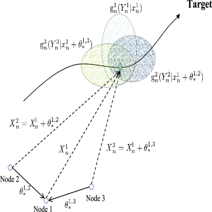
(a) Three node joint tracking example

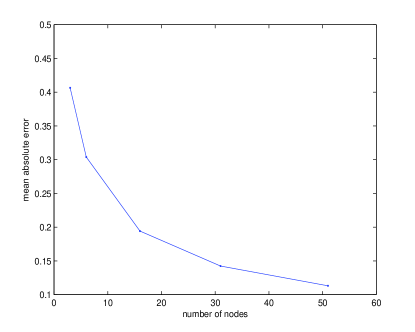
(b) Joint tracking error vs number of nodes

Figure 1: Left: a three node network tracking a target traversing its field of view. The trajectory of the target is shown with the solid line. Each node regards itself as the center of its local coordinate system. At time $n$ a measurement is registered by all three nodes. The ellipses show the support of the observation densities for the three nodes, i.e. the support of $g_{n}^{1}(Y_{n}^{1}|.)$ is defined as all $x_{n}^{1}$ such that $g_{n}^{1}(Y_{n}^{1}|x_{n}^{1})>0$ ; similarly for the rest. The filtering update step at node 1 will clearly benefit from the observations made by nodes 2 and 3. The localization parameters $\theta_{*}^{1,2}$, $\theta_{*}^{1,3}$ are the coordinates of node 1 in the local coordinate systems of node 2 and 3 respectively. While $X_{n}^{r}$ was defined to be the state of the target, which includes its velocity, for this illustration only, $X_{n}^{r}$ is to be understood as the position of the target at time $n$ w.r.t. the coordinate system of node $r$. Right: Average absolute tracking error is plotted against the number of nodes to illustrate the benefit of collaborative tracking. The results are obtained using a centralized implementation with 50 independent runs, $10^{4}$ time steps for a chain sensor network of different length and $A_{n}=B_{n}=Q_{n}=C_{n}^{i}=D_{n}^{i}=R_{n}^{i}=1$, $b_{n}^{i}=d_{n}^{i}=0$.

Figure 1 (a) illustrates a three node setting where a target is being jointly observed and tracked by three sensors. (Only the position of the target is shown.) At node 1, $X_{n}^{1}$ is defined relative to the local coordinate system of node 1 which regards itself as the origin. Similarly for nodes 2 and 3. We define $\theta_{\ast}^{i,j}$ to be the position of node $i$ in the local coordinate system of node $j$. This means that the vector $X_{n}^{i}$ relates to the local coordinate system of node $j$ as follows (see Figure 1):

$$X_{n}^{j}=X_{n}^{i}+\theta_{\ast}^{i,j}.$$

The localization parameters $\{\theta_{\ast}^{i,j}\}_{(i,j)\in\mathcal{E}}$ are static as the nodes are not mobile. We note the following obvious but important relationship: if nodes $i$ and $j$ are connected through intermediate nodes $j_{1},j_{2},\ldots,j_{m}$ then

$$\theta_{\ast}^{i,j}=\theta_{\ast}^{i,j_{1}}+\theta_{\ast}^{j_{1},j_{2}}+\theta_{\ast}^{j_{2},j_{3}}+\ldots+\theta_{\ast}^{j_{m-1},j_{m}}+\theta_{\ast}^{j_{m},j}.$$ (5)

This relationship is exploited to derive the distributed filtering and localization algorithms in the next section. We define $\theta_{\ast}^{i,j}$ so that the dimensions are the same as the target state vector. When the state vector is comprised of the position and velocity of the target, only the first and third components of $\theta_{\ast}^{i,j}$ are relevant while the other two are redundant and set to $\theta_{\ast}^{i,j}(2)=0$ and $\theta_{\ast}^{i,j}(4)=0$. Let

$$\theta_{\ast}\equiv\{\theta_{\ast}^{i,j}\}_{(i,j)\in\mathcal{E}},\quad\theta_{\ast}^{i,i}\equiv 0,$$ (6)

where $\theta_{\ast}^{i,i}$ for all $i\in\mathcal{V}$ is defined to be the zero vector.

Let $Y_{n}$ denote all the measurements received by the network at time $n$, i.e. $Y_{n}\equiv\{Y_{n}^{v}\}_{v\in\mathcal{V}}$. We also denote the sequence $(Y_{1},...,Y_{n})$ by $Y_{1:n}$. In the collaborative or joint filtering problem, each node $r$ computes the local filtering density:

$$p_{\theta_{\ast}}^{r}(x_{n}^{r}|Y_{1:n})\propto p_{\theta_{\ast}}^{r}(Y_{n}|x_{n}^{r})p_{\theta_{\ast}}^{r}(x_{n}^{r}|Y_{1:n-1}),$$ (7)

where $p_{\theta_{\ast}}^{r}(x_{n}^{r}|Y_{1:n-1})$ is the predicted density and is related to the filtering density of the previous time through the following prediction step:

$$p_{\theta_{\ast}}^{r}(x_{n}^{r}|Y_{1:n-1})=\int f_{n}(x_{n}^{r}|x_{n-1}^{r})p_{\theta_{\ast}}^{r}(x_{n-1}^{r}|Y_{1:n-1})dx_{n-1}^{r}.$$ (8)

The likelihood term is

$$p_{\theta_{\ast}}^{r}(Y_{n}|x_{n}^{r})=\prod\limits_{v\in\mathcal{V}}g_{n}^{v}(Y_{n}^{v}|x_{n}^{r}+\theta_{\ast}^{r,v}),$$ (9)

where the superscript on the densities indicate the coordinate system they are defined w.r.t. (and the node the density belongs to) while the subscript makes explicit the dependence on the localization parameters. Let also $\mu_{n|n-1}^{r}$ and $\mu_{n}^{r}$ denote the predicted and filtered mean of the densities $p_{\theta_{*}}^{r}(x_{n}^{r}|Y_{1:n-1})$ and $p_{\theta_{*}}^{r}(x_{n}^{r}|Y_{1:n})$ respectively, where the dependence on $\theta_{*}$ is suppressed in the notation. The prediction step in (8) can be implemented locally at each node without exchange of information, but the update step in (7) incorporates all the measurements of the network. Figure 1 (a) shows the support of the three observation densities as ellipses where the support of $g_{n}^{1}(Y_{n}^{1}|\cdot)$ is defined to be all $x^{1}$ such that $g_{n}^{1}(Y_{n}^{1}|\cdot)>0$; similarly for the rest. The filtering update step at node 1 can only include the observations made by nodes 2 and 3 provided the localization parameters $\theta_{\ast}^{1,2}$ and $\theta_{\ast}^{1,3}$ are known locally to node 1, since the likelihood $p_{\theta_{\ast}}^{1}(Y_{n}|x_{n}^{1})$ defined in (9) is

$$g_{n}^{1}(Y_{n}^{1}|x_{n}^{1})g_{n}^{2}(Y_{n}^{2}|x_{n}^{1}+\theta_{\ast}^{1,2})g_{n}^{3}(Y_{n}^{3}|x_{n}^{1}+\theta_{\ast}^{1,3}).$$

The term joint filtering is used since each sensor benefits from the observation made by all the other sensors. An illustration of the benefit w.r.t. the tracking error is in Figure 1 (b). We will show in Section 3 that it is possible to implement joint filtering in a truly distributed manner, i.e. each node executes a message passing algorithm (with communication limited only to neighboring nodes) that is scalable with the size of the network. However joint filtering hinges on knowledge of the localization parameters $\theta_{\ast}$ which are unknown a priori. In Section 4 we will propose distributed estimation algorithms to learn the localization parameters, which refine the parameter estimates as new data arrive. These proposed algorithms in this context are to the best of our knowledge novel.

2.1 Non-linear Model

Most tracking problems of practical interest are essentially non-linear non-Gaussian filtering problems. SMC methods, also known as Particle Filters, provide very good approximations to the filtering densities [29]. While it is possible to develop SMC methods for the problem presented here, the resulting algorithms require significantly higher computational cost. We refer the interested reader to [14, Chapter 9] for more details. In the interest of execution speed and simplicity, we employ the linearization procedure of the Extended Kalman filter (EKF) when dealing with a non-linear system. Specifically, let the distributed tracking system be given by the following model:

$$X_{n}^{r} =\phi_{n}(X_{n-1}^{r})+V_{n},$$ (10)

$$Y_{n}^{r} =\psi_{n}^{r}(X_{n}^{r})+W_{n}^{r},$$ (11)

where $\phi_{n}:\mathbb{R}^{4}\rightarrow\mathbb{R}^{4}$ and $\psi_{n}^{r}:\mathbb{R}^{4}\rightarrow\mathbb{R}^{d_{y}}$ are smooth continuous functions. At time $n$, each node will linearize its state and observation model about the filtered and predicted mean respectively. Specifically, a given node $r$ will implement:

$$X_{n}^{r}=\phi_{n}(\mu_{n-1}^{r}) +\nabla\phi_{n}(\mu_{n-1}^{r})(X_{n-1}^{r}-\mu_{n-1}^{r})+V_{n},$$ (12)

$$Y_{n}^{r}=\psi_{n}^{r}(\mu_{n|n-1}^{r}) +\nabla\psi_{n}^{r}(\mu_{n|n-1}^{r})(X_{n}^{r}-\mu_{n|n-1}^{r})+W_{n}^{r}.$$ (13)

where for a mapping $f:\mathbb{R}^{d}\rightarrow\mathbb{R}^{d}$, $\nabla f\equiv[\nabla f_{1},\ldots,\nabla f_{d}]^{\text{T}}$. Note that after linearization extra additive terms appear as seen in the setting described by equations (1)-(2).

2.2 Message passing

Assume at time $n$, the estimate of the localization parameters is $\theta_{n}=\{\theta_{n}^{i,j}\}_{(i,j)\in\mathcal{E}}$, with $\theta_{n}^{i,j}$ known to node $j$ only. To perform the prediction and update steps in (7)-(8) locally at each node a naive approach might require each node to access to all localization parameters $\theta_{n}$ and all the different model parameters $\{(C_{n}^{r},d_{n}^{r},R_{n}^{r})\}_{n\geq 1,r\in\mathcal{V}}$ . A scheme that requires all this information to be passed at every node would be inefficient. It would require a prohibitive amount of communication even for relatively few nodes and redundant computations would be performed at the different nodes. The core idea in this paper is to avoid this by storing the parameters in $\theta_{n}$ across the network and perform required computations only at the nodes where the parameters are stored. The results of these computations are then propagated in the network using an efficient message passing scheme.

1:  begin

2:  At $k=1,$ compute:

$$m_{n,1}^{i,j} =F_{n}^{i},$$ (14)

$$\ddot{m}_{n,1}^{i,j} =F_{n}^{i}\theta_{n}^{j,i}.$$ (15)

3:  for $k=2,...,K$ compute:

$$m_{n,k}^{i,j} =F_{n}^{i}+\sum\limits_{p\in\text{ne}(i)\setminus\{j\}}m_{n,k-1}^{p,i},$$ (16)

$$\ddot{m}_{n,k}^{i,j} =m_{n,k}^{i,j}\theta_{n}^{j,i}+\sum\limits_{p\in\text{ne}(i)\setminus\{j\}}\ddot{m}_{n,k-1}^{p,i}.$$ (17)

4:  endfor

5:  end

Algorithm 1 Generic message passing at time $n$

Message passing is an iterative procedure with $k=1,\ldots,K$ iterations for each time $n$ and is steered towards the development of a distributed Kalman filter, whose presentation is postponed for the next section. In Algorithm 1 we define a recursion of messages which are to be communicated between all pairs of neighboring nodes in both directions. Here ne$(i)$ denote the neighbors of node $i$ excluding node $i$ itself. At iteration $k$ the computed messages from node $i$ to $j$ are matrix and vector quantities of appropriate dimensions and are denoted as $m_{n,k}^{i,j}$ and $\ddot{m}_{n,k}^{i,j}$ respectively. The source node is indicated by the first letter of the superscript. Note that during the execution of Algorithm 1 time $n$ remains fixed and iteration $k$ should not be confused with time $n$. Clearly we assume that the sensors have the ability to communicate much faster than collecting measurements. We proceed with a simple (but key) lemma concerning the aggregations of sufficient statistics locally at each node.

Lemma 1

At time $n$, let $\left\{F_{n}^{v}\right\}_{v\in\mathcal{V}}$ be a collection of matrices where $F_{n}^{v}$ is known to node $v$ only, and consider the task of computing $\sum_{v\in\mathcal{V}}F_{n}^{v}$ and $\sum_{v\in\mathcal{V}}F_{n}^{v}\theta_{n}^{r,v}$ at each node $r$ of a network with a tree topology. Using Algorithm 1 and if $K$ is at least as large as the number of edges connecting the two farthest nodes in the network, then $\sum_{v\in\mathcal{V}}F_{n}^{v}=F_{n}^{r}+\sum\limits_{j\in\text{ne}(r)}m_{n,K}^{j,r}$ and $\sum_{v\in\mathcal{V}}F_{n}^{v}\theta_{n}^{r,v}=\sum\limits_{j\in\text{ne}(r)}\ddot{m}_{n,K}^{j,r}$.

(The proof, which uses (5), is omitted.) An additional advantage here is that if the network is very large, in the interest of speed one might be interested in settling with computing the presented sums only for a subset of nodes and thus use a smaller $K$. This also applies when a target traverses the field of view of the sensors swiftly and is visible only by few nodes at each time. Finally, a lower value for $K$ is also useful when cycles are present in order to avoid summing each $F_{n}^{i}$ more than once, albeit summing only over a subset of $\mathcal{V}$.

3 Distributed Joint Filtering

For a linear Gaussian system, the joint filter $p_{\theta}^{r}(x_{n}^{r}|Y_{1:n})$ at node $r$ is a Gaussian distribution with a specific mean vector $\mu_{n}^{r}$ and covariance matrix $\Sigma_{n}^{r}$. The derivation of the Kalman filter to implement $p_{\theta}^{r}(x_{n}^{r}|Y_{1:n})$ is standard upon noting that the measurement model at node $r$ can be written as $Y_{n}=C_{n}X_{n}^{r}+d_{n}+W_{n}$ where the $i$-th block of $Y_{n}$, $Y_{n}^{i}$, satisfies $Y_{n}^{i}=C_{n}^{i}(X_{n}^{r}+\theta^{r,i})+d_{n}^{i}+W_{n}^{i}$. However, there will be “non-local” steps due to the requirement that quantities $\underset{i\in\mathcal{V}}{\sum}(C_{n}^{i})^{\text{T}}(R_{n}^{i})^{-1}C_{n}^{i}$, $\underset{i\in\mathcal{V}}{\sum}(C_{n}^{i})^{\text{T}}(R_{n}^{i})^{-1}Y_{n}^{i}$ and $\underset{i\in\mathcal{V}}{\sum}(C_{n}^{i})^{\text{T}}(R_{n}^{i})^{-1}C_{n}^{i}\theta^{r,i}$ be available locally at node $r$. To solve this problem, we may use Lemma 1 with $F_{n}^{i}=(C_{n}^{i})^{\text{T}}(R_{n}^{i})^{-1}C_{n}^{i}$ and in order to compute $\underset{i\in\mathcal{V}}{\sum}(C_{n}^{i})^{\text{T}}(R_{n}^{i})^{-1}Y_{n}^{i}$ we will define $\dot{m}_{n,k}^{i,j}$ that is an additional message similar to $m_{n,k}^{i,j}$.

Recall that $b_{n}^{i},d_{n}^{i}$ are known local variables that arose due to linearization. Also to aid the development of the distributed on-line localization algorithms in Section 4, we assume that for the time being the localization parameter estimates $\{\theta_{n}\}_{n\geq 1}$ are time-varying and known to the relevant nodes they belong. For the case where that $b_{n}^{i},d_{n}^{i}=0$, we summarize the resulting distributed Kalman filter in Algorithm 2, which is to be implemented at every node of the network. Note that messages (18)-(20) are matrix and vector valued quantities and require a fixed amount of memory regardless of the number of nodes in the network. Also, the same rule for generating and combining messages are implemented at each node. The distributed Kalman filter presented here bears a similar structure to the one found in [30]. However, the message passing scheme is different and due to the application in mind we have extra terms relevant to the localization parameters.

1:  begin

2:  for $n\geq 1$:

3:  Let the localization parameter be $\theta_{n}$ and the set of collected measurements be $Y_{n}=\{Y_{n}^{v}\}_{v\in\mathcal{V}}$. Initialize messages $(m_{n,k}^{i,j},\dot{m}_{n,k}^{i,j},\ddot{m}_{n,k}^{i,j})$ and $(m_{n,k}^{j,i},\dot{m}_{n,k}^{j,i},\ddot{m}_{n,k}^{j,i})$ for all neighboring nodes $(i,j)\in\mathcal{E}$ as:

$$m_{n,1}^{i,j} =(C_{n}^{i})^{\text{T}}(R_{n}^{i})^{-1}C_{n}^{i},$$

$$\dot{m}_{n,1}^{i,j} =(C_{n}^{i})^{\text{T}}(R_{n}^{i})^{-1}Y_{n}^{i},$$

$$\ddot{m}_{n,1}^{i,j} =m_{n}^{i,j}\theta_{n}^{j,i},$$

4:  for $k=2,\ldots,K$ exchange the messages $(m_{n,k}^{i,j},\dot{m}_{n,k}^{i,j},\ddot{m}_{n,k}^{i,j})$ and $(m_{n,k}^{j,i},\dot{m}_{n,k}^{j,i},\ddot{m}_{n,k}^{j,i})$ defined below between all neighboring nodes $(i,j)\in\mathcal{E}$:

$$m_{n,k}^{i,j} =(C_{n}^{i})^{\text{T}}(R_{n}^{i})^{-1}C_{n}^{i}+\sum\limits_{p\in\text{ne}(i)\setminus\{j\}}m_{n,k-1}^{p,i},$$ (18)

$$\dot{m}_{n,k}^{i,j} =(C_{n}^{i})^{\text{T}}(R_{n}^{i})^{-1}Y_{n}^{i}+\sum\limits_{p\in\text{ne}(i)\setminus\{j\}}\dot{m}_{n,k-1}^{p,i},$$ (19)

$$\ddot{m}_{n,k}^{i,j} =m_{n}^{i,j}\theta_{n}^{j,i}+\sum\limits_{p\in\text{ne}(i)\setminus\{j\}}\ddot{m}_{n,k-1}^{p,i},$$ (20)

5:  end for

6:  Update the local filtering densities at each node $r\in\mathcal{V}$:

$$\mu_{n|n-1}^{r} =A_{n}\mu_{n-1}^{r},\quad\Sigma_{n|n-1}^{r}=A_{n}\Sigma_{n-1}^{r}A_{n}^{\text{T}}+Q_{n},$$ (21)

$$M_{n}^{r} =(\Sigma_{n|n-1}^{r})^{-1}+(C_{n}^{r})^{\text{T}}(R_{n}^{r})^{-1}C_{n}^{r}+\sum\limits_{i\in\text{ne}(r)}m_{n}^{i,r}$$ (22)

$$z_{n}^{r} =(\Sigma_{n|n-1}^{r})^{-1}\mu_{n|n-1}^{r}+(C_{n}^{r})^{\text{T}}(R_{n}^{r})^{-1}Y_{n}^{r}$$ (23)

$$+\sum\limits_{i\in\text{ne}(r)}\left(\dot{m}_{n}^{i,r}-\ddot{m}_{n}^{i,r}\right),$$

$$\Sigma_{n}^{r} =(M_{n}^{r})^{-1},\quad\mu_{n}^{r}=\Sigma_{n}^{r}z_{n}^{r},$$ (24)

7:  end for

8:  end

Algorithm 2 Distributed Filtering

In the case $b_{n}^{i},d_{n}^{i}\neq 0$ modifications to Algorithm 2 are as follows: in (21), to the right hand side of $\mu_{n|n-1}^{r}$, the term $b_{n}^{r}$ should be added and all instances of $Y_{n}^{r}$ should be replaced with $Y_{n}^{r}-d_{n}^{r}$. Therefore the assuming $b_{n}^{i},d_{n}^{i}=0$ does not compromise the generality of the approach. A direct application of this modification is the distributed EKF, which is obtained by adding the term $\phi_{n}(\mu_{n-1}^{r})-\nabla\phi_{n}(\mu_{n-1}^{r})\mu_{n-1}^{r}$ to the right hand side of $\mu_{n|n-1}^{r}$ in (21), and replacing all instances of $Y_{n}^{r}$ with $Y_{n}^{r}-\psi_{n}^{r}(\mu_{n|n-1}^{r})+\nabla\psi_{n}^{r}(\mu_{n|n-1}^{r})\mu_{n|n-1}^{r}$. In addition, one needs to replace $A_{n}$ with $\nabla\phi_{n}(\mu_{n-1}^{r})$.

4 Distributed Collaborative Localization

Following the discussion in Section 2 we will treat the sensor localization problem as a static parameter estimation problem for HMMs. The purpose of this section is to develop a fully decentralized implementation of popular Maximum Likelihood (ML) techniques for parameter estimation in HMMs. We will focus on two on-line ML estimation methods: Recursive Maximum Likelihood (RML) and Expectation-Maximization (EM). For the sake of completeness, we have added brief descriptions of these techniques in Section 7 of the appendix.

The core idea in our distributed ML formulation is to store the parameter $\theta_{n}=\{\theta_{n}^{i,j}\}_{(i,j)\in\mathcal{E}}$ across the network. Each node $r$ will use the available data $Y_{1:n}$ from every node to estimate $\theta_{\ast}^{r,j}$, which is the component of $\theta_{*}$ corresponding to edge $(r,j)$. This can be achieved computing at each node $r$ the ML estimate:

$$\widetilde{\theta}_{n}^{r,j}=\arg\max_{\theta^{r,j}\in\mathbb{R}^{4}}\log p_{\theta}^{r}(Y_{1:n}).$$ (25)

Note that each node maximizes its “local” likelihood function although all the data across the network is being used.

On-line parameter estimation techniques like the RML and on-line EM are suitable for sensor localization in surveillance applications because we expect a practically indefinite length of observations to arrive sequentially. For example, objects will persistently traverse the field of view of these sensors, i.e. the departure of old objects would be replenished by the arrival of new ones. A recursive procedure is essential to give a quick up-to-date parameter estimate every time a new set of observations is collected by the network. This is done by allowing every node $r$ to update the estimate of the parameter along edge $(r,j)$, $\theta_{n}^{r,j}$, according to a rule like

$$\theta_{n+1}^{r,j}=G_{n+1}^{r,j}(\theta_{n},Y_{n}),\qquad n\geq 1,$$ (26)

where $G_{n+1}^{r,j}$ is an appropriate function to be defined. Similarly each neighbor $j$ of $r$ will perform a similar update along the same edge only this time it will update $\theta_{n}^{j,r}$. While updating both parameters associated to each edge is redundant, it allows a fully decentralized implementation since no other communication is needed other than the messages defined in Algorithm 1. Alternatively one could assign both parameters of an edge to just one controlling node. For example in the three node network of Figure 1, the parameters of edge $(1,2)$, $\theta_{n}^{1,2}$ and $\theta_{n}^{2,1}$, could be assigned to node $2$, with the latter having at each time $n$ to update $\theta_{n}^{2,1}$ using an expression like (26) and then send $\theta_{n}^{1,2}=-\theta_{n}^{2,1}$ to node $1$.

4.1 Distributed RML

For distributed RML, each node $r$ updates the parameter of edge $(r,j)$ using

$$\theta_{n+1}^{r,j}=\theta_{n}^{r,j}+\gamma_{n+1}^{r}\left[\nabla_{\theta^{r,j}}\log\int p_{\theta}^{r}(Y_{n}|x_{n}^{r})p_{\theta}^{r}(x_{n}^{r}|Y_{1:n-1})dx_{n}^{r}\right]_{\theta=\theta_{n}},$$ (27)

where $\gamma_{n+1}^{r}$ is a step-size that should satisfy $\sum_{n}{\gamma_{n}^{r}}=\infty$ and $\sum_{n}{\left(\gamma_{n}^{r}\right)}^{2}<\infty$.

The gradient in (27) is w.r.t. $\theta^{r,j}$. The local joint predicted density $p_{\theta}^{r}(x_{n}^{r}|Y_{1:n-1})$ at node $r$ was defined in (8) and is a function of $\theta=\{\theta^{i,j}\}_{(i,j)\in\mathcal{E}}$, and likelihood term is given in (9). Also, the gradient is evaluated at $\theta_{n}=\{\theta_{n}^{i,j}\}_{(i,j)\in\mathcal{E}}$ while only $\theta_{n}^{r,j}$ is available locally at node $r$. The remaining values $\theta_{n}$ are stored across the network. All nodes of the network will implement such a local gradient algorithm with respect to the parameter associated to its adjacent edge. We note that (27) in the present form is not an on-line parameter update like (26) as it requires browsing through the entire history of observations. This limitation is removed by defining certain intermediate quantities that facilitate the online evaluation of this gradient in the spirit of [18, 19] (see in the Appendix for more details).

1:   begin

2:   for $n\geq 1$: let the current parameter estimate be $\theta_{n}$. Upon obtaining measurements $Y_{n}=\{Y_{n}^{v}\}_{v\in\mathcal{V}}$ the following filtering and parameter update steps are to be performed.

3:  Filtering step: Perform steps (3-6) in Algorithm 2.

4:  Parameter update: Each node $r\in\mathcal{V}$ of the network will update the following quantities for every edge $(r,j)\in\mathcal{E}$:

$$\dot{\mu}_{n|n-1}^{r,j} =A_{n}\dot{\mu}_{n-1}^{r,j},$$ (28)

$$\dot{z}_{n}^{r,j} =(\Sigma_{n|n-1}^{r})^{-1}\dot{\mu}_{n|n-1}^{r,j}-m_{n,K}^{j,r},$$ (29)

$$\dot{\mu}_{n}^{r,j} =(M_{n}^{r})^{-1}\dot{z}_{n}^{r,j}.$$ (30)

Upon doing so the localization parameter is updated:

$$\theta_{n+1}^{r,j} =\theta_{n}^{r,j}+\gamma_{n+1}^{r}[-(\dot{\mu}_{n|n-1}^{r,j})^{\text{T}}(\Sigma_{n|n-1}^{r})^{-1}\mu_{n|n-1}^{r}$$

$$+(\dot{z}_{n}^{r,j})^{\text{T}}(M_{n}^{r})^{-1}z_{n}^{r}+\dot{m}_{n,K}^{j,r}-\ddot{m}_{n,K}^{j,r}].$$

5:   end for

6:   end

Algorithm 3 Distributed RML

The distributed RML implementation for self-localization and tracking is presented in Algorithm 3, while the derivation of the algorithm is presented in the Appendix. The intermediate quantities (28)-(30) take values in $\mathbb{R}^{4\times 2}$ and may be initialized to zero matrices. For the non-linear model, when an EKF implementation is used for Algorithm 2, then Algorithm 3 remains the same.

4.2 Distributed on-line EM

We begin with a brief description of distributed EM in an off-line context and then present its on-line implementation. Given a batch of $T$ observations, let $p$ be the (off-line) iteration index and $\theta_{p}=\{\theta_{p}^{i,j}\}_{(i,j)\in\mathcal{E}}$ be the current estimate of $\theta_{\ast}$ after $p-1$ distributed EM iterations on the batch of observations $Y_{1:T}$. Each edge controlling node $r$ will execute the following E and M steps to update the estimate of the localization parameter for its edge. For iteration $p=1,2,\ldots$

$$\mbox{(E step) }Q^{r}(\theta_{p},\theta) =\int\log p_{\theta}^{r}(x_{1:T}^{r},Y_{1:T})p_{\theta_{p}}^{r}(x_{1:T}^{r}|Y_{1:T})dx_{1:T}^{r},$$

$$\mbox{(M step)}\qquad\theta_{p+1}^{r,j} =\arg\underset{\theta^{r,j}}{\max}\quad Q^{r}(\theta_{p},(\theta^{r,j},\theta_{p}^{-(r,j)})),$$

where $\theta_{p}^{-(r,j)}=\{\theta_{p}^{e}\}_{e\in\mathcal{E}\backslash(r,j)}$.

To show how the E-step can be computed we write $p_{\theta}^{r}(x_{1:T}^{r},Y_{1:T})$ as,

$$p_{\theta}^{r}(x_{1:T}^{r})p_{\theta}^{r}(Y_{1:T}|x_{1:T}^{r})=\prod\limits_{n=1}^{T}f_{n}(x_{n}^{r}|x_{n-1}^{r})p_{\theta}^{r}(Y_{n}|x_{n}^{r}),$$

where $p_{\theta}^{r}(Y_{n}|x_{n}^{r})$ was defined in (9). Note that $p_{\theta_{p}}^{r}(x_{1:T}^{r}|Y_{1:T})$ is a function of $\theta_{p}=\{\theta_{p}^{i,i^{\prime}}\}_{(i,i^{\prime})\in\mathcal{E}}$ (and not just $\theta_{p}^{r,j}$) and the $\theta$-dependance of $p_{\theta}^{r}(x_{1:T}^{r},Y_{1:T})$ arises through the likelihood term only as $p_{\theta}^{r}(x_{1:T}^{r})$ is $\theta$-independent. This means that in order to compute the E-step, it is sufficient to maintain the smoothed marginals:

$$p_{\theta}^{r}(x_{n}^{r}|Y_{1:T})\propto\int p_{\theta}^{r}(x_{1:T}^{r},Y_{1:T})dx_{1:T\backslash\{n\}}^{r},$$

where $1\leq n\leq T$ and $dx_{1:T\backslash\{n\}}^{r}$ means integration w.r.t. all variables except $x_{n}^{r}$. For linear Gaussian models this smoothed density is also Gaussian, with its mean and covariance denoted by $\mu_{n|T}^{r},\Sigma_{n|T}^{r}$ respectively.

The M-step is solved by setting the derivative of $Q^{r}(\theta_{p},(\theta^{r,j},\theta_{p}^{-(r,j)}))$ w.r.t. $\theta^{r,j}$ to zero. The details are presented in the Appendix and the main result is:

$$\nabla_{\theta^{r,j}}\int\log p_{\theta}^{r}(Y_{n}|x_{n}^{r})p_{\theta_{p}}^{r}(x_{n}^{r}|Y_{1:T})dx_{n}^{r}=\dot{m}_{n,K}^{j,r}-\ddot{m}_{n,K}^{j,r}-(m_{n,K}^{j,r})^{\text{T}}\mu_{n|T}^{r},$$

where $(m_{n,K}^{j,r},\dot{m}_{n,K}^{j,r},\ddot{m}_{n,K}^{j,r}),$ defined in (18)-(20), are propagated with localization parameter $\theta_{p}$ for all observations from time $1$ to $T$. Only $\ddot{m}_{n,K}^{j,r}$ is a function of $\theta^{r,j}$. To perform the M-step, the following equation is solved for $\theta^{r,j}$

$$(\sum_{n=1}^{T}m_{n,K}^{j,r})\theta^{r,j}=\sum_{n=1}^{T}(\dot{m}_{n,K}^{j,r}-(m_{n,K}^{j,r})^{\text{T}}\mu_{n|T}^{r}-\ddot{m}_{n,K}^{j,r}+\ddot{m}_{n,1}^{j,r}).$$ (31)

Note that $\theta^{r,j}$ is a function of quantities available locally to node $r$ only. The M-step can also be written as the following function:

$$\Lambda(\mathcal{S}_{T,1}^{r,j},\mathcal{S}_{T,2}^{r,j},\mathcal{S}_{T,3}^{r,j})=\left(\mathcal{S}_{T,2}^{r,j}\right)^{-1}\left(\mathcal{S}_{T,3}^{r,j}-\mathcal{S}_{T,1}^{r,j}\right),$$

where $\mathcal{S}_{T,1}^{r,j}$, $\mathcal{S}_{T,2}^{r,j}$, $\mathcal{S}_{T,3}^{r,j}$ are three summary statistics of the form:

$$\mathcal{S}_{T,l}^{r,j}=\frac{1}{T}\int\left(\sum_{n=1}^{T}s_{n,l}^{r,j}(x_{n}^{r},Y_{n})\right)p_{\theta_{p}}^{r}(x_{n}^{r}|Y_{1:T})dx_{n}^{r},\>l=1,2,3,$$

with $s_{n,l}^{r,j}$ being defined as follows:

$$s_{n,1}^{r,j}(x_{n}^{r},Y_{n}) = (m_{n,K}^{j,r})^{\text{T}}x_{n}^{r},\qquad s_{n,2}^{r,j}(x_{n}^{r},Y_{n})=m_{n,K}^{j,r},$$

$$\>s_{n,3}^{r,j}(x_{n}^{r},Y_{n}) = \dot{m}_{n,K}^{j,r}-\ddot{m}_{n,K}^{j,r}+\ddot{m}_{n,1}^{j,r}.$$

Note that for this problem $s_{n,2}^{r,j}$ and $s_{n,3}^{r,j}$ are state independent.

An on-line implementation of EM follows by computing recursively running averages for each of the three summary statistics, which we will denote as $\mathcal{S}_{n,1}^{r,j},\mathcal{S}_{n,2}^{r,j},\mathcal{S}_{n,3}^{r,j}$. At each time $n$ these will be used at every node $r$ to update $\theta^{r,j}$ using $\theta_{n+1}^{r,j}=\Lambda(\mathcal{S}_{n,1}^{r,j},\mathcal{S}_{n,2}^{r,j},\mathcal{S}_{n,3}^{r,j})$. Note that $\Lambda$ is the same function for every node. The on-line implementation of distributed EM is found in Algorithm 4. All the steps are performed with quantities available locally at node $r$ using the exchange of messages as detailed in Algorithm 2. The derivation of the recursions for $\mathcal{S}_{n,1}^{r,j}$, $\mathcal{S}_{n,2}^{r,j}$, $\mathcal{S}_{n,3}^{r,j}$ are based on (42)-(43) in the Appendix. Here $\gamma_{n}^{r}$ is a step-size satisfying the same conditions as in RML and $\theta_{0}$ can be initialized arbitrarily, e.g. the zero vector. Finally, it has been reported in [31] that it is usually beneficial for the first few epochs not to perform the M step in (32) and allow a burn-in period for the running averages of the summary statistics to converge.

1:   begin

2:   for $n\geq 1$: let the current parameter estimate be $\theta_{n}$. Upon obtaining measurements $Y_{n}=\{Y_{n}^{v}\}_{v\in\mathcal{V}}$ the following filtering and parameter update steps are to be performed.

3:  Filtering step: Perform steps (3-6) in Algorithm 2. Also compute

$$\tilde{\Sigma}_{n}^{r}=\left(\Sigma_{n-1}^{r}+A_{n}^{\text{T}}Q_{n}^{-1}A_{n}\right)^{-1}.$$

4:  Parameter update: Each node $r\in\mathcal{V}$ of the network will update the following quantities for every edge $(r,j)\in\mathcal{E}$:

$$H_{n}^{r,j} = \gamma_{n}^{r}(m_{n,K}^{j,r})^{\text{T}}+(1-\gamma_{n}^{r})H_{n-1}^{r,j}\left(\tilde{\Sigma}_{n}^{r}\right)^{-1}A_{n}^{\text{T}}Q_{n}^{-1},$$

$$h_{n}^{r,j} = (1-\gamma_{n}^{r})\left(H_{n-1}^{r,j}\left(\tilde{\Sigma}_{n}^{r}\right)^{-1}\left(\Sigma_{n-1}^{r}\right)^{-1}\mu_{n-1}^{r}+h_{n-1}^{r,j}\right),$$

$$\mathcal{S}_{n,1}^{r,j} = H_{n}^{r,j}\mu_{n}^{r}+h_{n}^{r,j}.$$

$$\mathcal{S}_{n,2}^{r,j} = \gamma_{n}^{r}m_{n,K}^{j,r}+\left(1-\gamma_{n}^{r}\right)\mathcal{S}_{n-1,2}^{r,j},$$

$$\mathcal{S}_{n,3}^{r,j} = \gamma_{n}^{r}(\dot{m}_{n,K}^{j,r}-\ddot{m}_{n,K}^{j,r}+\ddot{m}_{n,1}^{j,r})+\left(1-\gamma_{n}^{r}\right)\mathcal{S}_{n-1,3}^{r,j},$$

Upon doing so the localization parameter is updated:

$$\theta_{n+1}^{r,j}=\Lambda(\mathcal{S}_{n,1}^{r,j},\mathcal{S}_{n,2}^{r,j},\mathcal{S}_{n,3}^{r,j}).$$ (32)

5:   end for

6:   end

Algorithm 4 Distributed on-line EM

5 Numerical Examples

The performance of the distributed RML and EM algorithms are studied using a Linear Gaussian and a non-linear model. For both cases the hidden target is given in (1) with $V_{n}=B\widetilde{V}_{n},$ where $\widetilde{V}_{n}$ is zero mean Gaussian additive noise with variance $\widetilde{Q}_{n}$, and

$$A_{n}=\left[\begin{array}[]{cccc}1&\tau&0&0\\ 0&1&0&0\\ 0&0&1&\tau\\ 0&0&0&1\end{array}\right],\quad B=\left[\begin{array}[]{cc}\frac{\tau^{2}}{2}&0\\ \tau&0\\ 0&\frac{\tau^{2}}{2}\\ 0&\tau\end{array}\right],\quad\widetilde{Q}_{n}=\sigma_{x}^{2}I,$$

and $I$ is the identity matrix. For the linear model the observations are given by (2) with

$$C_{n}^{r}=\alpha^{r}\left[\begin{array}[]{cccc}1&0&0&0\\ 0&0&1&0\end{array}\right],\quad R_{n}^{r}=\sigma_{y}^{2}I,$$

where $\alpha^{r}$ are constants different for each node and are assigned randomly from the interval $[0.75,1.25]$. For the non-linear model we will use the bearings-only measurement model. In this model at each node $r$, the observation $Y_{n}^{r}$ is:

$$Y_{n}^{r}=tan^{-1}(X_{n}^{r}(1)/X_{n}^{r}(3))+W_{n}^{r}.$$

with $W_{n}^{r}\overset{i.i.d.}{\sim}\mathcal{N}(0,{0.35}^{2})$. For the remaining parameters we set $\tau=0.01$, $\sigma_{x}$ $=$1 and $\theta_{0}^{r,j}=0$ for all $(r,j)\in\mathcal{E}$ . In Figure 2 we show three different sensor networks for which we will perform numerical experiments.

In Figure 3 we present various convergence plots for each of these networks for $\sigma_{y}=0.5$. We plot both dimensions of the errors $\theta_{\ast}^{r,j}-\theta_{n}^{r,j}$ for three cases:

• in (a) and (d) we use distributed RML and on-line EM respectively for the network of Figure 2(a) and the linear Gaussian model.

• in (b) and (e) we use distributed RML for the bearings only tracking model and the networks of Figures 2(a) and 2(b) respectively. Local linearization as discussed in Sections 2.1, 3 and 4.1 was used to implement the distributed RML algorithm. We remark that we do not apply the online EM to problems where the solution to the M-step cannot be expressed analytically as some function $\Lambda$ of summary statistics.

• in (c) and (f) we use distributed RML and on-line EM for respectively for the network of Figure 2(c) and the linear Gaussian model. In this case we used $K=2$.

All errors converge to zero. Although both methods are theoretically locally optimal when performing the simulations we did not observe significant discrepancies in the errors for different initializations. For both RML and on-line EM we used for $n\leq 10^{3}$ a constant but small step-size, $\gamma_{n}^{r}=\gamma=4\times 10^{-3}$ and $0.025$ respectively. For the subsequent iterations we set $\gamma_{n}^{r}=\gamma(n-10^{3}){}^{-0.8}$ . Note that if the step-size decreases too quickly in the first time steps, these algorithms might converge too slowly. In the plots of Figure 3 one can notice that the distributed RML and EM algorithms require comparable amount of time to converge with the RML being usually faster. For example in Figures 3 (a) and (d) we observe that RML requires around $1000$ iterations to converge whereas on-line EM requires approximately 2000 iterations. We note that the converge rate also depends on the specific network used, the value of $K$ and the simulation parameters.

To investigate this further we varied $K$ and $\frac{\sigma_{x}}{\sigma_{y}}$ and recorded the root mean squared error (RMSE) for $\theta_{n}$ obtained for the network of Figure 2(b) using $50$ independent runs. For the RMSE at time $n$ we will use $\sqrt{\frac{1}{50\left|\mathcal{E}\right|}\sum_{e\in\mathcal{E}}\sum_{m=1}^{50}\left\|\theta_{\ast}^{r,j}-\theta_{n,m}^{r,j}\right\|_{2}^{2}}$, where $\theta_{n,m}^{r,j}$ denotes the estimated parameter at epoch $n$ obtained from the $m$-th run. The results are plotted in Figure 4 for different cases:

• in (a) and (b) for $\frac{\sigma_{x}}{\sigma_{y}}=2$ we show the RMSE for $K=2,4,8,12$. We observe that in every case the RMSE keeps reducing as $n$ increases. Both algorithms behave similarly with the RML performing better and showing quicker convergence. One expects that observations beyond your near immediate neighbors are not necessary to localize adjacent nodes and hence the good performance for small values of $K$.

• in (b) and (c) we show the RMSE for RML and on-line EM respectively when $\frac{\sigma_{x}}{\sigma_{y}}=10,1,0.5,0.1$. We observe that EM seems to be slightly more accurate for lower values of $\frac{\sigma_{x}}{\sigma_{y}}$ with the reverse holding for higher values of the ratio.

In each run the same step-size was used as before except for RML and $\frac{\sigma_{x}}{\sigma_{y}}=10$, where we had to reduce the step size by a factor of $10$.

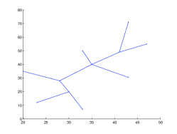
(a) 11 node sensor network

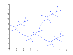
(b) 44 node sensor network

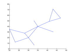
(c) 11 node sensor network with cycles

Figure 2: Various sensor networks of different size and topology.

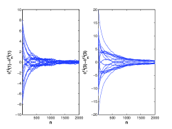
(a) RML for tree network

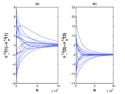
(b) Nonlinear RML for tree network

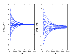
(c) RML for network with cycles

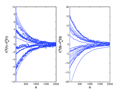
(d) EM for tree network

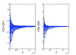
(e) Nonlinear RML for large network

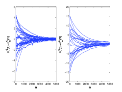
(f) EM for network with cycles

Figure 3: The convergence of the localization parameters’ estimates to $\theta_{\ast}^{r,j}$ is demonstrated using appropriate error plots for various sensor networks. Left: Parameter error after each iteration for each edge of the medium sensor network of Fig. 2(a). In each subfigure left and right columns show the errors in the x- and y- coordinates respectively; (a) is for RML and (d) is for EM. Middle: Same errors when using RML for the nonlinear bearings-only observation model; (b) is for medium sized network of Fig. 2(a) and (e) for the large network of Fig. 2(b). Right: Same errors for network with cycles seen in Fig 2(c); (c) for RML and (f) for EM.

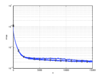
(a) RML for different K

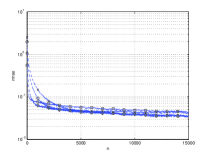
(b) EM for different K

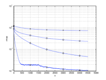
(c) RML for different $\frac{\sigma_{x}}{\sigma_{y}}$

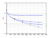
(d) EM for different $\frac{\sigma_{x}}{\sigma_{y}}$

Figure 4: Comparison of distributed RML and on-line EM. (a) (and (b) resp.): RMSE for RML (and on-line EM resp.) against $n$ for $K=$ $2$ ($\square$), $4$ ($\diamond$), $8$ ($\circ$), 12($\times$). (c) (and (d) resp.): RMSE for RML (and on-line EM resp.) for $\frac{\sigma_{x}}{\sigma_{y}}=$ $10$ ($\square$), $1$ ($\diamond$), $0.5$ ($\circ$), $0.1$($\times$).

6 Conclusion

We have presented a method to perform collaborative tracking and self-localization. We exploited the fact that different nodes collect measurements of a common target. This idea has appeared previously in [9, 10], both of which use a Bayesian inference scheme for the localization parameters. We remark that our distributed ML methods appear simpler to implement than these Bayesian schemes as the messages here are nothing more than the appropriate summary statistics for computing the filtering density and performing parameter updates. There is good empirical evidence that the distributed implementations of ML proposed in this paper are stable and do seem to settle at reasonably accurate estimates. A theoretical investigation of the properties of the schemes would be an interesting but challenging extension. Finally, as pointed out by one referee, another interesting extension would be to develop consensus versions of Algorithm 1 in the spirit of gossip algorithms in [32] or the aggregation algorithm of [33] which might be particularly relevant for networks with cycles, which are dealt with here by using an appropriate value for $K$.

7 Maximum likelihood parameter estimation

This section does not pertain to sensor localization specifically but to the general problem of static parameter estimation in HMMs using ML. Thus to avoid confusion with the localization problem a different font is used the notation. Consider a HMM where $\{\mathsf{X}_{n}\}_{n\geq 1}$ is the hidden state-process and $\{\mathsf{Y}_{n}\}_{n\geq 1}$ is the observed process each taking values in taking values in $\mathbb{R}^{d_{x}}$ and $\mathbb{R}^{d_{y}}$ respectively. For the transition density for $\{\mathsf{X}_{n}\}_{n\geq 1}$, we have $\mathsf{X}_{n+1}|\mathsf{X}_{n}=\mathsf{x}_{n}\sim\mathsf{f}(\cdot|\mathsf{x}_{n})$. The observation model, $\mathsf{Y}_{n}|\mathsf{X}_{n}=\mathsf{x}_{n}\sim\mathsf{g}_{\vartheta}(\cdot|\mathsf{x}_{n})$ is parametrized by $\vartheta\in\Theta\>(\subset\mathbb{R}^{d_{\vartheta}})$. The true static parameter generating the sequence of observations is $\vartheta_{\ast}$ and is to be learned from the observed data $\{\mathsf{Y}_{n}\}_{n\geq 1}$. The ML parameter estimate is the maximizing argument of the log-likelihood of the observed data up to time $n$: $\tilde{\vartheta}_{n}=\arg\max_{\vartheta\in\Theta}\log p_{\vartheta}(\mathsf{Y}_{1:n})$. Here $p_{\vartheta}(\mathsf{Y}_{1:n})$ denotes the joint density of $\mathsf{Y}_{1:n}$ and the subscript makes explicit the value of the parameter used to compute this density.

For a long observation sequence we are interested in a recursive parameter estimation procedure in which the data is run through once sequentially. If $\vartheta_{n}$ is the estimate of the model parameter after $n$ observations, a recursive method would update the estimate to $\vartheta_{n+1}$ after receiving the new data $\mathsf{Y}_{n}$. For example, consider the following update scheme:

$$\vartheta_{n+1}=G_{n+1}(\vartheta_{n},\mathsf{Y}_{n}),\qquad n\geq 1.$$ (33)

where $G_{n+1}$ is an appropriate function to be defined. This scheme was originally suggested by [34, 35] when $\{\mathsf{X}_{n}\}_{n\geq 1}$ is not a Markov chain but rather an independent and identically distributed (i.i.d.) sequence.

7.1 Recursive Maximum Likelihood (RML)

To motivate a suitable choice for $G_{n+1}(\vartheta_{n},\mathsf{Y}_{n})$ for estimating the parameters of a HMM, consider the following recursion:

$$\vartheta_{n+1}=\vartheta_{n}+\gamma_{n+1}\left.\nabla\log p_{\vartheta}(\mathsf{Y}_{n}|\mathsf{Y}_{1:n-1})\right|_{\vartheta=\vartheta_{n}}.$$ (34)

where $\{\gamma_{n}\}$ is the step-size sequence that should satisfy the following constraints: $\sum_{n}\gamma_{n}=\infty$ and $\sum_{n}\gamma_{n}^{2}<\infty$. One possible choice would be $\gamma_{n}=n^{-\alpha}$, $0.5<\alpha<1$. Here $p_{\vartheta}(\mathsf{Y}_{n}|\mathsf{Y}_{1:n-1})$ is the conditional density of $\mathsf{Y}_{n}$ given $\mathsf{Y}_{1:n-1}\$ and the subscript makes explicit the value of the parameter used to compute this density. Upon receiving $\mathsf{Y}_{n}$, $\vartheta_{n}$ is updated in the direction of ascent of the conditional density of this new observation. The algorithm in the present form is not suitable for online implementation due to the need to evaluate the gradient of $\log p_{\vartheta}(\mathsf{Y}_{n}|\mathsf{Y}_{1:n-1})$ (w.r.t. $\vartheta$) at $\vartheta=\vartheta_{n}$. Doing so would require browsing through the entire history of observations. This limitation is removed by defining certain intermediate quantities that facilitate the online evaluation of this gradient [18, 19].

In particular, assume that from the previous iteration of the RML, one has computed $p_{n}(\mathsf{x}_{n})\approx\left.p_{\vartheta}(\mathsf{x}_{n}|\mathsf{Y}_{1:n-1})\right|_{\vartheta=\vartheta_{n}}$ and $\dot{p}_{n}(\mathsf{x}_{n})\approx\left.\nabla p_{\vartheta}(\mathsf{x}_{n}|\mathsf{Y}_{1:n-1})\right|_{\vartheta=\vartheta_{n}.}$, where $(p_{n},\dot{p}_{n})$ are approximations of the predicted density and its gradient evaluated at $\vartheta=\vartheta_{n}$. The RML is initialized with an arbitrary value for $\vartheta_{1}$, $p_{1}(\mathsf{x}_{1})=p_{\vartheta_{1}}(\mathsf{x}_{1})$, which is the prior distribution for $\mathsf{X}_{1}$ and $\dot{p}_{1}(\mathsf{x}_{1})=\left.\nabla p_{\vartheta}(\mathsf{x}_{1})\right|_{\vartheta=\vartheta_{1}}$, i.e. the gradient of this prior which could be zero if it does not depend on $\vartheta$. Then the online version of (34), which is the RML procedure of [18, 19], proceeds as follows. Given the new observation $\mathsf{Y}_{n}$, update the parameter:

$$\vartheta_{n+1}=\vartheta_{n}+\gamma_{n+1}\left(\int\mathsf{g}_{\vartheta_{n}}(\mathsf{Y}_{n}|\mathsf{x}_{n})p_{n}(\mathsf{x}_{n})d\mathsf{x}_{n}\right)^{-1}\left(\int\mathsf{\dot{g}}_{\vartheta_{n}}(\mathsf{Y}_{n}|\mathsf{x}_{n})p_{n}(\mathsf{x}_{n})d\mathsf{x}_{n}+\int\mathsf{g}_{\vartheta_{n}}(\mathsf{Y}_{n}|\mathsf{x}_{n})\dot{p}_{n}(\mathsf{x}_{n})d\mathsf{x}_{n}\right)$$ (35)

where $n\geq 1$ and $\mathsf{\dot{g}}_{\vartheta^{\prime}}(\mathsf{y}|\mathsf{x})\equiv\left.\nabla_{\vartheta}\mathsf{g}_{\vartheta}(\mathsf{y}|\mathsf{x})\right|_{\vartheta=\vartheta^{\prime}}$. In (34), the desired gradient is the ratio of the terms $\left.p_{\vartheta}(\mathsf{Y}_{n}|\mathsf{Y}_{1:n-1})\right|_{\vartheta=\vartheta_{n}}$ and $\left.\nabla p_{\vartheta}(\mathsf{Y}_{n}|\mathsf{Y}_{1:n-1})\right|_{\vartheta=\vartheta_{n}}$. This ratio is approximated in the fraction on the right-hand side of (35). After computing (35), one may update $(p_{n},\dot{p}_{n})$ to $(p_{n+1},\dot{p}_{n+1})$ for the next RML iteration. Specific expressions for this update may be found for example in [14, Section 8.2.1] or [18]. The recursive propagation of $(p_{n},\dot{p}_{n})$ implicitly involves the previous values of the parameter, i.e. $\vartheta_{1:n}$, and hence are only approximations to $\left.p_{\vartheta}(\mathsf{x}_{n}|\mathsf{Y}_{1:n-1})\right|_{\vartheta=\vartheta_{n+1}}$, $\left.\nabla p_{\vartheta}(\mathsf{x}_{n}|\mathsf{Y}_{1:n-1})\right|_{\vartheta=\vartheta_{n}}$ respectively. It has been shown in [18] that the solution of RML converges to the true ML estimator without any loss of efficiency. For more details on the convergence of RML for HMMs we refer the reader to [18].

7.2 On-line Expectation-Maximization (EM)

We begin this section with a brief description of Expectation-Maximization (EM) [36] and then present its on-line implementation. EM is an iterative off-line algorithm for learning $\vartheta_{\ast}$, which consists of repeating a two step procedure given a batch of $T$ observations. Let $p$ be the (off-line) iteration index. The first step, the expectation or E-step, computes

$$Q(\vartheta_{p},\vartheta)=\int\log p_{\vartheta}(\mathsf{x}_{1:T},\mathsf{Y}_{1:T})p_{\vartheta_{p}}(\mathsf{x}_{1:T}|\mathsf{Y}_{1:T})d\mathsf{x}_{1:T}.$$ (36)

The second step is the maximization or M-step that updates the parameter $\vartheta_{p}$,

$$\vartheta_{p+1}=\arg\max\quad Q(\vartheta_{p},\vartheta)$$ (37)

Upon the completion of an E and M step, the likelihood surface is ascended, i.e. $p_{\vartheta_{p+1}}(\mathsf{Y}_{1:T})\geq p_{\vartheta_{p}}(\mathsf{Y}_{1:T})$ [36]. When $p_{\theta}(\mathsf{x}_{1:T},\mathsf{Y}_{1:T})$ is in the exponential family, which is the case of linear Gaussian state-space models, this procedure can be implemented exactly. Then the E-step is equivalent to computing a summary statistic of the form

$$\mathcal{S}_{T}^{\vartheta_{p}}=\frac{1}{T}\int\left(\sum_{n=1}^{T}s_{n}\left(\mathsf{x}{}_{n-1:n},\mathsf{Y}_{n}\right)\right)p_{\vartheta_{p}}(\mathsf{x}_{1:T}|\mathsf{Y}_{1:T})d\mathsf{x}_{1:T}.$$ (38)

where $s_{n}:\mathbb{R}^{d_{x}}\times\mathbb{R}^{d_{x}}\times\mathbb{R}^{d_{y}}\rightarrow\mathbb{R}^{\kappa}$. In addition, the maximizing argument of $Q(\vartheta_{p},\vartheta)$ can be characterized in this case explicitly through a suitable function $\Lambda:\mathbb{R}^{\kappa}\rightarrow\Theta$, i.e.

$$\vartheta_{p}=\Lambda\left(\mathcal{S}_{T}^{\vartheta_{p}}\right).$$ (39)

Note that in the usual EM setup one has to compute (38) for every iteration $p$ of the algorithm.

It is also possible to propose an on-line version of the EM algorithm. This was originally proposed for finite state-space and linear Gaussian models in [21, 37, 20] and for exponential family models in [22, 31]. In the online implementation of the EM, running averages of the sufficient statistics are computed [20, 21, 22]. Let $\{\vartheta_{m}\}_{1\leq m\leq n}$ be the sequence of parameter estimates of the online EM algorithm computed sequentially based on $\mathsf{Y}_{1:n-1}$. When $\mathsf{Y}_{n}$ is received, we compute

$$\mathcal{S}_{n}=\gamma_{n}\text{ }\int s_{n}\left(\mathsf{x}{}_{n-1:n}\right)p_{\vartheta_{1:n}}(\mathsf{x}{}_{n-1:n}|\mathsf{Y}_{1:n})d\mathsf{x}{}_{n-1:n}$$

(40)

where the subscript $\vartheta_{1:n}$ on $p_{\vartheta_{1:n}}(\mathsf{x}_{1:T}|\mathsf{Y}_{1:n})$ indicates that the posterior density is being computed sequentially using the parameter $\vartheta_{m}$ at time $m\leq n$. The step sizes $\left\{\gamma_{n}\right\}_{n\geq 1}$ need to satisfy $\sum_{n}\gamma_{n}=\infty$ and $\sum_{n}\gamma_{n}^{2}<\infty$ as in the RML case. For the M-step one uses the same maximization step (39) used in the batch version

$$\vartheta_{n+1}=\Lambda\left(\mathcal{S}_{n}\right).$$ (41)

The recursive calculation of $\mathcal{S}_{n}$ can be achieved by setting $V_{1}\left(\mathsf{x}_{0}\right)=0$ and computing

$$V_{n}\left(\mathsf{x}_{n}\right) = \int\left\{\gamma_{n}\text{ }s_{n}\left(\mathsf{x}_{n-1},\mathsf{x}_{n}\right)+\left(1-\gamma_{n}\right)\text{ }V_{n-1}\left(\mathsf{x}_{n-1}\right)\right\}$$ (42)

$$\times p_{\vartheta_{1:n}}\left(\left.\mathsf{x}_{n-1}\right|\mathsf{Y}_{1:n-1},\mathsf{x}_{n}\right)d\mathsf{x}_{n-1}$$

and

$$\mathcal{S}_{n}=\int V_{n}\left(\mathsf{x}_{n}\right)p_{\vartheta_{1:n}}(\mathsf{x}_{n}|\mathsf{Y}_{1:n})d\mathsf{x}_{n}.$$ (43)

For finite state-space and linear Gaussian models, all the quantities appearing in this algorithm can be calculated exactly [20, 21, 31].

8 Distributed RML derivation

Let $\theta_{n}=\{\theta_{n}^{i,j}\}_{(i,j)\in\mathcal{E}}$ be the estimate of the true parameter $\theta_{\ast}$ given the available data $Y_{1:n-1}$. Consider an arbitrary node $r$ and assume it controls edge $(r,j)$. At time $n$, we assume the following quantities are available: $(\dot{\mu}_{n-1}^{r,j}=\left.\nabla_{\theta^{r,j}}\mu_{n-1}^{r}\right|_{\theta=\theta_{n}},\left.\mu_{n-1}^{r}\right|_{\theta=\theta_{n}},\Sigma_{n-1}^{r})$. The first of these quantities is the derivative of the conditional mean of the hidden state at node $r$ given $Y_{1:n-1}$, i.e. $\left.\nabla_{\theta^{r,j}}\int x_{n-1}^{r}p_{\theta}^{r}(x_{n-1}^{r}|Y_{1:n-1})dx_{n-1}^{r}\right|_{\theta=\theta_{n}}$. This quantity is a function of the localization parameter $\theta_{n}$. $\Sigma_{n-1}^{r}$ is the variance of the distribution $\left.p_{\theta}^{r}(x_{n-1}^{r}|Y_{1:n-1})\right|_{\theta=\theta_{n}}$ and is independent of the localization parameter. The log-likelihood in (27) evaluates to:

$$\log p_{\theta}^{r}(Y_{n}|Y_{1:n-1})=-\frac{1}{2}\underset{i\in\mathcal{V}}{\sum}(Y_{n}^{i}-C_{n}^{i}\theta^{r,i})^{T}R_{n}^{i}{}^{-1}(Y_{n}^{i}-C_{n}^{i}\theta^{r,i})$$

$$-\frac{1}{2}\mu_{n|n-1}^{r}{}^{\text{T}}(\Sigma_{n|n-1}^{r})^{-1}\mu_{n|n-1}^{r}+\frac{1}{2}(z_{n}^{r})^{\text{T}}(M_{n}^{r})^{-1}z_{n}^{r}+const$$

where all $\theta$ independent terms have been lumped together in the term ‘const’. (Refer to Algorithm 2 for the definition of the quantities in this expression.) Differentiating this expression w.r.t. $\theta^{r,j}$ yields

$$\nabla_{\theta^{r,j}}\log p_{\theta}^{r}(Y_{n}|Y_{1:n-1}) =-(\nabla_{\theta^{r,j}}\mu_{n|n-1}^{r})^{\text{T}}(\Sigma_{n|n-1}^{r})^{-1}\mu_{n|n-1}^{r}$$

$$+(\nabla_{\theta^{r,j}}z_{n}^{r})^{\text{T}}(M_{n}^{r})^{-1}z_{n}^{r}+\underset{i\in\mathcal{V}}{\sum}(\nabla_{\theta^{r,j}}\theta^{r,i})^{\text{T}}(C_{n}^{i})^{\text{T}}(R_{n}^{i})^{-1}(Y_{n}^{i}-C_{n}^{i}\theta^{r,i}).$$

(27) requires $\nabla_{\theta^{r,j}}\log p_{\theta}^{r}(Y_{n}|Y_{1:n-1})$ to be evaluated at $\theta=\theta_{n}$. Using the equations (21)-(24) and the assumed knowledge of $(\dot{\mu}_{n-1}^{r,j},\left.\mu_{n-1}^{r}\right|_{\theta=\theta_{n}},\Sigma_{n-1}^{r})$ we can evaluate the derivatives on the right-hand side of this expression:

$$\dot{\mu}_{n|n-1}^{r,j} =\left.\nabla_{\theta^{r,j}}\mu_{n|n-1}^{r}\right|_{\theta=\theta_{n}}=A_{n}\dot{\mu}_{n-1}^{r,j},$$ (44)

$$\dot{z}_{n}^{r,j} =\left.\nabla_{\theta^{r,j}}z_{n}^{r}\right|_{\theta=\theta_{n}}=(\Sigma_{n|n-1}^{r})^{-1}\dot{\mu}_{n|n-1}^{r,j}-\underset{i\in\mathcal{V}}{\sum}(C_{n}^{i})^{\text{T}}(R_{n}^{i})^{-1}C_{n}^{i}\left.\nabla_{\theta^{r,j}}\theta^{r,i}\right|_{\theta=\theta_{n}},$$ (45)

$$\dot{\mu}_{n}^{r,j} =\left.\nabla_{\theta^{r,j}}\mu_{n}^{r}\right|_{\theta=\theta_{n}}=(M_{n}^{r})^{-1}\dot{z}_{n}^{r,j}.$$ (46)

Using property (5) we note that for the set of vertices $i$ for which the path from $r$ to $i$ includes edge $(r,j)$, $\nabla_{\theta^{r,j}}\theta^{r,i}=I$ (the identity matrix) whereas for the rest $\nabla_{\theta^{r,j}}\theta^{r,i}=0$. For all the nodes $i$ for which $\nabla_{\theta^{r,j}}\theta^{r,i}=I$, let them form a sub tree $(\mathcal{V}_{rj}^{\prime},\mathcal{E}_{rj}^{\prime})$ branching out from node $j$ away from node $r$. Then the last sum in the expression for $\left.\nabla_{\theta^{r,j}}\log p_{\theta}^{r}(Y_{n}|Y_{1:n-1})\right|_{\theta=\theta_{n}}$ evaluates to,

$$\underset{i\in\mathcal{V}_{rj}^{\prime}}{\sum}(C_{n}^{i})^{\text{T}}(R_{n}^{i})^{-1}(Y_{n}^{i}-C_{n}^{i}\theta_{n}^{r,i})=\dot{m}_{n,K}^{j,r}-\ddot{m}_{n,K}^{j,r},$$

where messages $(\dot{m}_{n,K}^{j,r},\ddot{m}_{n,K}^{j,r})$ were defined in Algorithms 2. Similarly, we can write the sum in the expression for $\dot{z}_{n}^{r,j}$ as $m_{n,K}^{j,r}$ (again refer to Algorithms 2) to obtain

$$\dot{z}_{n}^{r,j}=(\Sigma_{n|n-1}^{r})^{-1}\dot{\mu}_{n|n-1}^{r,j}-m_{n,K}^{j,r}.$$ (47)

To conclude, the approximations to $(\dot{\mu}_{n}^{r,j}=\left.\nabla_{\theta^{r,j}}\mu_{n}^{r}\right|_{\theta=\theta_{n+1}},\left.\mu_{n}^{r}\right|_{\theta=\theta_{n+1}},\Sigma_{n}^{r})$ for the subsequent RML iteration, i.e. (27) at time $n=n+1,$ are given by

$$\dot{\mu}_{n}^{r,j}=(M_{n}^{r})^{-1}\dot{z}_{n}^{r,j}$$

while $(\left.\mu_{n}^{r}\right|_{\theta=\theta_{n+1}},\Sigma_{n}^{r})$ are given by (21)-(24). The approximation to $\left.\nabla_{\theta^{r,j}}\mu_{n}^{r}\right|_{\theta=\theta_{n+1}}$ follows from differentiating (24). $(\dot{\mu}_{n}^{r,j},\left.\mu_{n}^{r}\right|_{\theta=\theta_{n+1}})$ are only approximations because they are computed using the previous values of the parameters, i.e. $\theta_{1:n}$.

9 Distributed EM derivation

For the off-line EM approach, once a batch of $T$ observations have been obtained, each node $r$ of the network that controls an edge will execute the following E and M step iteration $n$,

$$Q^{r}(\theta_{p},\theta) =\int\log p_{\theta}^{r}(x_{1:T}^{r},Y_{1:T})p_{\theta_{p}}^{r}(x_{1:T}^{r}|Y_{1:T})dx_{1:T}^{r},$$

$$\theta_{p+1}^{r,j} =\arg\underset{\theta^{r,j}\in\Theta}{\max}Q^{r}(\theta_{p},(\theta^{r,j},\{\theta^{e},e\in\mathcal{E}\backslash(r,j)\})),$$

where it is assumed that node $r$ controls edge $(r,j)$. The quantity $p_{\theta_{p}}^{r}(x_{1:T}^{r}|Y_{1:T})$ is the joint distribution of the hidden states at node $r$ given all the observations of the network from time $1$ to $T$ and is given up to a proportionality constant,

$$p_{\theta_{p}}^{r}(x_{1:T}^{r})p_{\theta_{p}}^{r}(Y_{1:T}|x_{1:T}^{r})=\prod\limits_{n=1}^{T}f_{n}(x_{n}^{r}|x_{n-1}^{r})p_{\theta_{p}}^{r}(Y_{n}|x_{n}^{r}),$$

where $p_{\theta_{p}}^{r}(Y_{n}|x_{n}^{r})$ was defined in (9). Note that $p_{\theta_{p}}^{r}(x_{1:T}^{r},Y_{1:T})$ (and hence $p_{\theta_{p}}^{r}(x_{1:T}^{r}|Y_{1:T})$) is a function of $\theta_{p}=\{\theta_{p}^{i,i^{\prime}}\}_{(i,i^{\prime})\in\mathcal{E}}$ and not just $\theta_{p}^{r,j}$. Also, the $\theta$-dependence of $p_{\theta}^{r}(x_{1:T}^{r},Y_{1:T})$ arises through the likelihood term only as $p_{\theta}^{r}(x_{1:T}^{r})$ is $\theta$ independent. Note that

$$\sum_{v\in\mathcal{V}}\log g_{n}^{v}(Y_{n}^{v}|x_{n}^{r}+\theta^{r,v}) =\sum_{v\in\mathcal{V}}c_{n}^{v}-\frac{1}{2}\sum_{v\in\mathcal{V}}(Y_{n}^{v}-C_{n}^{v}\theta^{r,v})^{\text{T}}(R_{n}^{v})^{-1}(Y_{n}^{v}-C_{n}^{v}\theta^{r,v})$$

$$+(x_{n}^{r})^{\text{T}}\sum_{v\in\mathcal{V}}(C_{n}^{v})^{\text{T}}(R_{n}^{v})^{-1}(Y_{n}^{v}-C_{n}^{v}\theta^{r,v})-\frac{1}{2}(x_{n}^{r})^{\text{T}}\left[\sum_{v\in\mathcal{V}}(C_{n}^{v})^{\text{T}}(R_{n}^{v})^{-1}C_{n}^{v}\right]x_{n}^{r}$$

where $c_{n}^{v}$ is a constant independent of $\theta$. Taking the expectation w.r.t. $p_{\theta_{n}}^{r}(x_{n}^{r}|Y_{1:T})$ gives

$$\int\log p_{\theta}^{r}(Y_{n}|x_{n}^{r})p_{\theta_{p}}^{r}(x_{n}^{r}|Y_{1:T})dx_{n}^{r} =-\frac{1}{2}\sum_{v\in\mathcal{V}}\left[(Y_{n}^{v}-C_{n}^{v}\theta^{r,v})^{\text{T}}(R_{n}^{v})^{-1}(Y_{n}^{v}-C_{n}^{v}\theta^{r,v})\right]$$

$$-(\mu_{n|T}^{r})^{\text{T}}\sum_{v\in\mathcal{V}}(C_{n}^{v})^{\text{T}}(R_{n}^{v})^{-1}C_{n}^{v}\theta^{r,v}+\text{const}$$

where all terms independent of $\theta^{r,j}$ have been lumped together as ’const’ and $\mu_{n|T}^{r}$ is the mean of $x_{n}^{r}$ under $p_{\theta_{p}}^{r}(x_{n}^{r}|Y_{1:T})$. Taking the gradient w.r.t. $\theta^{r,j}$ and following the steps in the derivation of the distributed RML we obtain

$$\nabla_{\theta^{r,j}}\int\log p_{\theta}^{r}(Y_{n}|x_{n}^{r})p_{\theta_{p}}^{r}(x_{n}^{r}|Y_{1:T})dx_{n}^{r}=\dot{m}_{n,K}^{j,r}-\ddot{m}_{n,K}^{j,r}-(m_{n,K}^{j,r})^{\text{T}}\mu_{n|T}^{r}$$

where $(m_{n,K}^{j,r},\dot{m}_{n,K}^{j,r},\ddot{m}_{n,K}^{j,r})$ is defined in (18)-(20). Only $\ddot{m}_{n,K}^{j,r}$ is a function of $\theta^{r,j}$. Now to perform the M-step, we solve

$$\left(\sum_{n=1}^{T}m_{n,K}^{j,r}\right)\theta^{r,j}=\sum_{n=1}^{T}\left(\dot{m}_{n,K}^{j,r}-(m_{n,K}^{j,r})^{\text{T}}\mu_{n|T}^{r}-\sum\limits_{j^{\prime}\in\text{ne}(j)\setminus\{r\}}\ddot{m}_{n,K-1}^{j^{\prime},j}\right).$$

Note that $\theta^{r,j}$ can be recovered by standard linear algebra and so far $\theta^{r,j}$ is solved by quantities available locally to node $r$ and $j$. One can use the fact that $\sum\limits_{j^{\prime}\in\text{ne}(j)\setminus\{r\}}\ddot{m}_{n,K-1}^{j^{\prime},j}=\ddot{m}_{n,K}^{j,r}-\ddot{m}_{n,1}^{j,r}$ to so that the M-step can be performed with quantities available locally to node $r$ only. Recall that $\sum_{n=1}^{T}\mu_{n|T}^{r}=\int\left(\sum_{n=1}^{T}x_{n}^{r}\right)p_{\theta_{p}}^{r}(x_{1:T}^{r}|Y_{1:T})dx_{1:T}^{r}.$ This implies directly that three summary statistics are needed for node $r$ to update $\theta^{r,j}$. These should be defined using:

$$s_{n,1}^{r,j}(x_{n}^{r},Y_{n})=(m_{n,K}^{j,r})^{\text{T}}x_{n}^{r},\>s_{n,2}^{r,j}(x_{n}^{r},Y_{n})=m_{n,K}^{j,r},\>s_{n,3}^{r,j}(x_{n}^{r},Y_{n})=\dot{m}_{n,K}^{j,r}-\ddot{m}_{n,K}^{j,r}+\ddot{m}_{n,1}^{j,r},$$

where $s_{n,1}^{r}$, $s_{n,3}^{r}$ are each functions of $x_{n}^{r}$ and $Y_{n}$ via $\mu_{n|T}^{r}$ and $\dot{m}_{n,K}^{j,r}-\ddot{m}_{n,K}^{j,r}+\ddot{m}_{n,1}^{j,r}$ respectively. The summary statistics can be written in the form of (38) as follows:

$$\mathcal{S}_{T,1}^{r,j^{,\theta_{p}}} = \frac{1}{T}\int\left(\sum_{n=1}^{T}(m_{n,K}^{j,r})^{\text{T}}x_{n}^{r}\right)p_{\theta_{p}}^{r}(x_{1:T}^{r}|Y_{1:T})dx_{1:T}^{r},$$

$$\mathcal{S}_{T,2}^{r,j^{\theta_{p}}} = \frac{1}{T}\sum_{n=1}^{T}m_{n,K}^{j,r},\quad\mathcal{S}_{T,3}^{r,j^{\theta_{p}}}=\frac{1}{T}\sum_{n=1}^{T}\left(\dot{m}_{n,K}^{j,r}-\ddot{m}_{n,K}^{j,r}+\ddot{m}_{n,1}^{j,r}\right),$$

and the M-step function becomes $\Lambda(s_{1},s_{2},s_{3})=s_{2}^{-1}\left(s_{3}-s_{1}\right),$ where $s_{1},s_{2},s_{3}$ correspond to each of the three summary statistics. Note that $\Lambda$ is the same function for every node.

We will now proceed to the on-line implementation. Let at time $n$ the estimate of the localization parameter be $\theta_{n}$. Following the description of Section 7.2, for every $r\in\mathcal{V}$ and $(r,j)\in\mathcal{E}$, let $\mathcal{S}_{n,1}^{r,j}$, $\mathcal{S}_{n,2}^{r,j}$, $\mathcal{S}_{n,3}^{r,j}$ be the running averages (w.r.t $n$) for $\mathcal{S}_{T,1}^{r,j^{\theta_{p}}}$, $\mathcal{S}_{T,2}^{r,j^{\theta_{p}}}$ and $\mathcal{S}_{T,3}^{r,j^{\theta_{p}}}$ respectively. The recursions for $\mathcal{S}_{n,2}^{r,j}$, $\mathcal{S}_{n,3}^{r,j}$ are trivial:

$$\mathcal{S}_{n,2}^{r,j}=\gamma_{n}^{r}m_{n,K}^{j,r}+\left(1-\gamma_{n}^{r}\right)\mathcal{S}_{n-1,2}^{r,j},\>\mathcal{S}_{n,3}^{r,j}=\gamma_{n}^{r}(\dot{m}_{n,K}^{j,r}-\ddot{m}_{n,K}^{j,r}+\ddot{m}_{n,1}^{j,r})+\left(1-\gamma_{n}^{r}\right)\mathcal{S}_{n-1,3}^{r,j},$$

where $\left\{\gamma_{n}^{r}\right\}_{n\geq 1}$ needs to satisfy $\sum_{n\geq\text{1}}\gamma_{n}^{r}=\infty$ and $\sum_{n\geq 1}\left(\gamma_{n}^{r}\right)^{2}<\infty$. For $\mathcal{S}_{n,1}^{r,j}$, we will use (42)-(43). We first set $V_{0}^{r,j}\left(x_{0}^{r}\right)=0$ and define the recursion

$$V_{n}^{r,j}\left(x_{n}^{r}\right)=\gamma_{n}^{r}(m_{n,K}^{j,r})^{\text{T}}x_{n}^{r}+\left(1-\gamma_{n}^{r}\right)\int\text{ }V_{n-1}^{r,j}\left(x_{n-1}^{r}\right)p_{\theta_{1:n}}^{r}\left(\left.x_{n-1}^{r}\right|Y_{1:n-1},x_{n}^{r}\right)dx_{n-1}^{r}.$$ (48)

Using standard manipulations with Gaussians we can derive that $p_{\theta_{1:n}}^{r}\left(\left.x_{n-1}^{r}\right|Y_{1:n-1},x_{n}^{r}\right)$ is itself a Gaussian density with mean and variance denoted by $\tilde{\mu}_{n}^{r}(x_{n}),\widetilde{\Sigma}_{n}^{r}$ respectively, where

$$\tilde{\Sigma}_{n}^{r}=\left(\Sigma_{n-1}^{r}+A_{n}^{\text{T}}Q_{n}^{-1}A_{n}\right)^{-1},\>\widetilde{\mu}_{n}^{r}(x_{n})=\tilde{\Sigma}_{n}^{r}\left(\left(\Sigma_{n-1}^{r}\right)^{-1}\mu_{n-1}^{r}+A_{n}^{\text{T}}Q_{n}^{-1}x_{n}\right).$$

It is then evident that (48) becomes $V_{n}^{r,j}\left(x_{n}^{r}\right)=H_{n}^{r,j}x_{n}^{r}+h_{n}^{r,j}$, with:

$$H_{n}^{r,j} = \gamma_{n}^{r}(m_{n,K}^{j,r})^{\text{T}}+(1-\gamma_{n}^{r})H_{n-1}^{r,j}\left(\tilde{\Sigma}_{n}^{r}\right)^{-1}A_{n}^{\text{T}}Q_{n}^{-1},$$

$$h_{n}^{r,j} = (1-\gamma_{n}^{r})\left(H_{n-1}^{r,j}\left(\tilde{\Sigma}_{n}^{r}\right)^{-1}\left(\Sigma_{n-1}^{r}\right)^{-1}\mu_{n-1}^{r}+h_{n-1}^{r,j}\right),$$

where $H_{0}^{r,j}=0$ and $h_{0}^{r,j}=0$. Finally, the recursive calculation of $\mathcal{S}_{n,1}^{r,j}$ is achieved by computing

$$\mathcal{S}_{n,1}^{r,j}=\int V_{n}^{r,j}\left(x_{n}^{r}\right)p_{\theta_{0:n}}^{r}(x_{n}^{r}|Y_{0:n})dx_{n}^{r}=H_{n}^{r,j}\mu_{n}^{r}+h_{n}^{r,j}.$$

Again all the steps are performed locally at node $r$, which can update parameter $\theta^{r,j}$ using $\theta_{n+1}^{r,j}=\Lambda(\mathcal{S}_{n,1}^{r,j},\mathcal{S}_{n,2}^{r,j},\mathcal{S}_{n,3}^{r,j}).$

References

- [1] N. Patwari, J. N. Ash, S. Kyperountas, A. O. Hero III, R. L. Moses, and N. S. Correal, “Locating the nodes: cooperative localization in wireless sensor networks,” IEEE Signal Processing Magazine, vol. 22, no. 4, pp. 54–69, July 2005.
- [2] K. Plarre and P. Kumar, “Tracking objects with networked scattered directional sensors,” EURASIP Journal on Advances in Signal Processing, vol. 2008, p. 74, 2008.
- [3] N. B. Priyantha, H. Balakrishnan, E. D. Demaine, and S. Teller, “Mobile-assisted localization in wireless sensor networks,” in Proc. 24th Annual Joint Conference of the IEEE Computer and Communications Societies INFOCOM 2005, vol. 1, 13–17 March 2005, pp. 172–183.
- [4] A. T. Ihler, J. W. Fisher III, R. L. Moses, and A. S. Willsky, “Nonparametric belief propagation for self-localization of sensor networks,” IEEE Journal on Selected Areas in Communications, vol. 23, no. 4, pp. 809–819, April 2005.
- [5] R. L. Moses, D. Krishnamurthy, and R. Patterson, “A self-localization method for wireless sensor networks,” Eurasip Journal on Applied Signal Processing, Special Issue on Sensor Networks, vol. 2003, no. 4, pp. 348–358, Mar. 2003.
- [6] M. Vemula, M. F. Bugallo, and P. M. Djuric, “Sensor self-localization with beacon position uncertainty.” Signal Processing, pp. 1144–1154, 2009.
- [7] V. Cevher and J. H. McClellan, “Acoustic node calibration using moving sources,” IEEE Transactions on Aerospace and Electronic Systems, vol. 42, no. 2, pp. 585–600, 2006.
- [8] X. Chen, A. Edelstein, Y. Li, M. Coates, M. Rabbat, and A. Men, “Sequential monte carlo for simultaneous passive device-free tracking and sensor localization using received signal strength measurements,” in Proc. IEEE/ACM Int. Conf. on Information Processing in Sensor Networks, Chicago, IL, 2011.
- [9] S. Funiak, C. Guestrin, M. Paskin, and R. Sukthankar, “Distributed localization of networked cameras,” in Proc. Fifth International Conference on Information Processing in Sensor Networks IPSN 2006, 2006, pp. 34–42.
- [10] C. Taylor, A. Rahimi, J. Bachrach, H. Shrobe, and A. Grue, “Simultaneous localization, calibration, and tracking in an ad hoc sensor network,” in Proc. Fifth International Conference on Information Processing in Sensor Networks IPSN 2006, 2006, pp. 27–33.
- [11] Y. Baryshnikov and J. Tan, “Localization for anchoritic sensor networks,” in Proc. 3rd IEEE International Conference on Distributed Computing in Sensor Systems (DCOSS ’07), Santa Fe, New Mexico, USA, 18–20 June 2007.
- [12] N. Kantas, S. S. Singh, and A. Doucet, “Distributed online self-localization and tracking in sensor networks,” in Proc. 5th International Symposium on Image and Signal Processing and Analysis ISPA 2007, 27–29 Sept. 2007, pp. 498–503.
- [13] J. Pearl, Probabilistic Reasoning in Intelligent Systems: Networks of Plausible Inference. Morgan-Kauffman, 1988.
- [14] N. Kantas, “Stochastic decision making for general state space models,” Ph.D. dissertation, University of Cambridge, February 2009.
- [15] O. Cappé, E. Moulines, and T. Rydén, Inference in hidden Markov models. Springer, 2005.
- [16] R. Elliott, L. Aggoun, and J. Moore, Hidden Markov models: estimation and control. Springer-Verlag, 1995.
- [17] U. Holst and G. Lindgren, “Recursive estimation in mixture models with markov regime,” IEEE Transactions on Information Theory, vol. 37, no. 6, pp. 1683–1690, Nov. 1991.
- [18] F. LeGland and L. Mevel, “Recursive estimation in hidden markov models,” in Proc. 36th IEEE Conference on Decision and Control, vol. 4, 10–12 Dec. 1997, pp. 3468–3473.
- [19] I. B. Collings and T. Ryden, “A new maximum likelihood gradient algorithm for on-line hidden markov model identification,” in Proc. IEEE International Conference on Acoustics, Speech and Signal Processing, vol. 4, 12–15 May 1998, pp. 2261–2264.
- [20] J. J. Ford, “Adaptive hidden markov model estimation and applications,” Ph.D. dissertation, Dept. of Systems Engineering, Australian National University, 1998.
- [21] R. Elliott, J. Ford, and J. Moore, “On-line consistent estimation of hidden markov models,” Department of Systems Engineering, Australian National University, Tech. Rep., 2000.
- [22] O. Cappe and E. Moulines, “Online em algorithm for latent data models,” Journal of the royal statistical society. Series B (Methodological), vol. 71, p. 593, 2009.
- [23] R. D. Nowak, “Distributed em algorithms for density estimation and clustering in sensor networks,” IEEE Transactions on Signal Processing, Special Issue on Signal Processing in Networking, vol. 51, no. 8, pp. 2245–2253, Aug. 2003.
- [24] M.-A. Sato and S. Ishii, “On-line EM Algorithm for the Normalized Gaussian Network,” Neural Comp., vol. 12, no. 2, pp. 407–432, 2000.
- [25] D. Blatt and A. Hero, “Distributed maximum likelihood estimation for sensor networks,” in Proc. Int. Conf. Acoustics, Speech, Signal Processing, 2004, pp. 929–932.
- [26] N. N. Okello and S. Challa, “Joint sensor registration and track-to-track fusion for distributed trackers,” IEEE Transactions on Aerospace and Electronic Systems, vol. 40, no. 3, pp. 808–823, July 2004.
- [27] J. Vermaak, S. Maskell, and M. Briers, “Online sensor registration,” in Proc. IEEE Aerospace Conference, 5–12 March 2005, pp. 2117–2125.
- [28] L. Xiao, S. Boyd, and S. Lall, “A scheme for robust distributed sensor fusion based on average consensus,” in Proc. Fourth International Symposium on Information Processing in Sensor Networks IPSN 2005, 15 April 2005, pp. 63–70.
- [29] A. Doucet, N. de Freitas, and N. Gordon, Eds., Sequential Monte Carlo Methods in Practise. New York: Springer, 2001.
- [30] S. Grime and H. Durrant-Whyte, “Data fusion in decentralized sensor networks,” Control Engineering Practice, vol. 2, no. 1, pp. 849–863, 1994.
- [31] O. Cappe, “Online em algorithm for hidden markov models,” Journal Computational Graphical Statistics, vol. to appear, 2011.
- [32] D. Kempe, A. Dobra, and J. Gehrke, “Gossip-based computation of aggregate information,” in In Proc. 44th Annual IEEE Symposium on Foundations of Computer Science, 2003., 2003, pp. 482–491.
- [33] D. Bertsekas and J. Tsitsiklis, Parallel and distributed computation. Prentice Hall Inc.m, Old Tappan, NJ (USA), 1989.
- [34] D. M. Titterington, “Recursive parameter estimation using incomplete data,” Journal of the Royal Statistical Society of London, Series B (Methodological), vol. 46, no. 2, pp. 257–267, 1984.
- [35] D. M. Titterington and J.-M. Jiang, “Recursive estimation procedures for missing-data problems,” Biometrika, vol. 70, no. 3, pp. 613–624, Dec 1983.
- [36] A. P. Dempster, N. M. Laird, and D. B. Rudin, “Maximum likelihood from incomplete data via the em algorithm,” Journal of the Royal Statistical Society of London, Series B (Methodological), vol. 39, pp. 1–38, 1977.
- [37] R. J. Elliott, J. J. Ford, and J. B. Moore, “On-line almost-sure parameter estimation for partially observed discrete-time linear systems with known noise characteristics,” International Journal of Adaptive Control and Signal Processing, vol. 16, no. 6, pp. 435–453, 2002.