Designing Incoherent Dictionaries for Compressed Sensing: Algorithm Comparison

Chapter 1 Compressed Sensing

1.1 What is Compressed Sensing?

Let us consider the following image which will be used extensively throughout this introduction.

Figure 1.1: Lena

To insert this image into the report I pointed my editor to the file called Lena.jpg which was automatically added to the text. Let us take a closer view at the file. The size of the image is $512\times 512$ pixels. Each pixel contains an integer number in the range between 0 and 255 hence, there is one byte (8 bits) of storage reserved to keep the value of each pixel. Simple calculations show that the file should occupy at least $512\times 512\times 1=262144$ bytes, however, the size of the file is only 44791 bytes. To understand where the difference came from let us review the way this file arrived to my computer. First, the person portrayed in the image was photographed by an analogous camera. Then, the film or the photograph was scanned by a digital scanner to form a digital image that is already suitable for use by the computer. Note that the size of this image is $512\times 512$, assuming that the original film had dimensions of $6\times 6$ centimeters we conclude that the resolution of the scanning (sampling) process was about 85 samples per centimeter (in both directions). Sampling rate is important if we want to reconstruct the original analog image. Such a reconstruction is possible if we sample with the sufficiently high rate, as defined by the Nyquist-Shannon theorem. However, we shall return to our image which currently requires 262144 bytes of storage. In the next step it undergoes a process called compression. One of the most common compression techniques for images is known under the name JPEG compression. We describe here a very primitive version of this compression method which, nevertheless, contains the most important details.

The images is splitted into square blocks and each block undergoes the two-dimensional discrete cosine transfrom (DCT), as depicted in Figure1.2

Figure 1.2: 2D DCT on $64\times 64$ patches

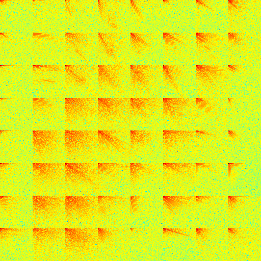
Note that the most energy (reddish colors) is concentrated in a relatively small fraction of the DCT coefficients, thus the coefficients that are close to zero are discarded and we end up with a significantly smaller number of the DCT coefficients that represent the original image without significant visual artifacts. The original JPEG compression does not stops here; it has a number of further steps. Those are not important for our discussion. I would like to draw your attention to the two important effects we achieved by discarding some of the DCT coefficients. First, we, obviously, lost some information about the original image, thus the compression method is lossy. Second, we used only a small number of the original coefficients which means that we switched to a sparse representation of the original patches in the DCT base. The latter property is of paramount importance as we shall see in the sequel.

It turns out that sampling signals with high resolution may be wastfull in case that the signals of interset are compressible or, alternatively, are known to have a sparse representation in some basis. Compressed Sensing is an emerging framework dealing with efficient ways to sample such signals.

1.2 Formal definition

Consider a signal $x\in\mathbb{R}^{n}$ that is known to have a sparse representation over a certain dictionary $D\in\mathbb{R}^{n\times k}$, i.e,.

$$x=D\theta,$$

where $\|\theta\|_{0}\leq S\ll n$. The classical sampling methods would require $n$ samples per signal. The Compressed Sensting, on the other hand, suggests to replace these $n$ direct samples with $m$ inderect ones by measuring linear projections of $x$ defined by a projection matrix $P\in\mathbb{R}^{m\times n}$

$$y=Px,$$

such that $S<m\ll n$. That means that instaed of sensing $n$ elements of the original signal we can sense it directly in compressed form, by sampling a relatively small number of linear projections

$$y_{i}=\left\langle p_{i},x\right\rangle.$$

The main question with whether the original signal can be reconstructed from this insufficient number of samples. Surprisingly, the answer is yes. In this paper we are going to review the methods to design efficient projections, but, meanwhile we present some of the notorious projections used in practice in Figure 1.3.

$\left\langle\begin{matrix}\quad\includegraphics[width=130.08731pt]{figs/lena512}&,&\includegraphics[width=130.08731pt]{figs/bigpixel}\quad\end{matrix}\right\rangle$

(a) big pixel

$\left\langle\begin{matrix}\quad\includegraphics[width=130.08731pt]{figs/lena512}&,&\includegraphics[width=130.08731pt]{figs/lineintegral}\quad\end{matrix}\right\rangle$

(b) line projection (tomography)

$\left\langle\begin{matrix}\quad\includegraphics[width=130.08731pt]{figs/lena512}&,&\includegraphics[width=130.08731pt]{figs/sinusoid}\quad\end{matrix}\right\rangle$

(c) sinusoid (MRI)

$\left\langle\begin{matrix}\quad\includegraphics[width=130.08731pt]{figs/lena512}&,&\includegraphics[width=130.08731pt]{figs/randomprojection}\quad\end{matrix}\right\rangle$

(d) random projection

Figure 1.3: Graphical representation of common projections.

1.3 Designing optimal projections

In this section we consider the case when the dictionary $D$ is fixed while the projection matrix $P$ can be arbitrary. Hence, we would like to design $P$ that will suit us in the best way. Before we proceed with the design let us define an important property that characterizes a dictionary $D$.

Definition 1.

For a dictionary $D$, its mutual coherence is defined as the largest absolute and normalized inner product between the different columns of $D$

$$\mu(D)=\max_{i\not=j}\frac{|d_{i}^{T}d_{j}|}{\|d_{i}\|\|d_{j}\|},$$

where $d_{i}$ denotes the $i$-th column of $D$.

An alternative definition of the mutual coherence is via the largest (by magnitude) off-diagonal value of the Gram matrix

$$G=\tilde{D}^{T}\tilde{D},$$

where $\tilde{D}$ denotes the “normalized” version of $D$, i.e., the columns of $D$ are scaled to unity (in $l_{2}$ norm).

The mutual coherence provides a quantitative measure of how far are the columns of $D$ from being orthogonal to each other. It also has a strong influence on the theoretical analysis of worst case scenarios, as implied by the following theorem.

Theorem 2.

Given a signal $x=D\hat{\theta}$ such that

$$\|\hat{\theta}\|_{0}<\frac{1}{2}\left(1+\frac{1}{\mu(D)}\right)$$

then the following three results hold:

1. The vector $\hat{\theta}$ is necessarily the sparsest one to describe $x$, i.e., it is the unique solution of

   $$\min_{\theta}\|\theta\|_{0}\mbox{ s.t. }x=D\theta.$$

2. The Basis Pursuit (BP) algorithm that approximates the exact solution $\hat{\theta}$ by solving the linear problem

   $$\min_{\theta}\|\theta\|_{1}\mbox{ s.t. }x=D\theta,$$

   is guaranteed to find the exact solution $\hat{\theta}$.

3. The Orthogonal Matching Pursuit (OMP) that is a greed approximate algorithm which iteratively solve the least squares problem

   $$\|x-D\theta\|_{2}^{2}$$

   for only one component of $\theta$ per iteration is also guaranteed to obtain the unique solution $\hat{\theta}$.

With the aforementioned properties of $\mu$ there is an obvious reason to design the projection matrix $P$ in a way that minimizes the mutual coherence $\mu(PD)$. Note the treatment of the mutual coherence has addressed only the worst case behavior so far. This analysis does not provide any insight into the “average” behavior of the pursuit algorithms. It is possible that relaxing the requirement on the maximal $\mu$ value, that, on the other hand, leads to decrease in the average $\mu$ may lead to better average performance of the pursuit algorithms. Following this idea Elad introduced another measure which is defined as follows.

Definition 3.

For a dictionary $D$, its $t$-average mutual coherence is defined as the average of all absolute and normalized inner products between different columns in $D$ (denoted as $g_{ij}$) that are above $t$. Formally it reads

$$\mu_{t}(D)=\frac{\sum_{i\not=j}(|g_{ij}|>t)\cdot|g_{ij}|}{\sum_{i\not=j}(|g_{ij}|>t)}.$$

For $t=0$, we obtain a simple average of the absolute entries of $\tilde{G}$. As the value of $t$ grows, we obtain that $\mu_{t}(D)$ grows and approaches $\mu(D)$ from below. It is also evident from the definition that $\mu_{t}(D)\geq t$.

1.3.1 Elad’s method

Along with the definition given above, Elad, who followed the approach of Dhillon et al., also suggested and iterative algorithm that that tries to minimize the value $\mu_{t}(PD)$ with respect to $P$, assuming that both the dictionary $D$ and parameter $t$ are given and fixed the algorithm may be formalized as follows.

• Objective: Minimize $\mu_{t}(PD)$ with respect to $P$.

  Input: Use the following parameters:

  • $t$ or $t\%$ - fixed or relative threshold,

  • $D$ - the dictionary

  • $p$ - number of measurements

  • $\gamma$ - down-scaling factor

  • $Iter$ - number of iterations

  Initialization: set $P_{0}\in\mathbb{R}^{m\times n}$ to an arbitrary matrix

  Loop: Set $q=0$ (iteration counter) and repeat $Iter$ iterations:

  1. Normalize: Normalize the columns of $P_{q}D$ and obtain the effective dictionary $\tilde{D}_{q}$.

  2. Compute Gram Matrix: $G_{q}=\tilde{D}_{q}^{T}\tilde{D}_{q}$.

  3. Set Threshold: If mode of operation is fixed, use $t$ as threshold. Otherwise, chose $t$ such that $t\%$ of the off-diagonal elements in $G_{q}$ is above it.

  4. Shrink: Update the Gram matrix and obtain $\hat{G}_{q}$ by

     $$\hat{g}_{ij}=\begin{cases}\gamma g_{ij}&|g_{ij}|\geq t\\ \gamma t\cdot\mathrm{sign}(g_{ij})&t>|g_{ij}|\geq\gamma t\\ g_{ij}&\gamma t>|g_{ij}|\end{cases}.$$

  5. Reduce Rank: Apply SVD and force the rank of $\hat{G}_{q}$ to be equal to $m$.

  6. Squared-Root: Build the squared-root of $\hat{G}_{q}$, $S_{q}^{T}S_{q}=\hat{G}_{q}$, where $S_{q}$ is of size $m\times k$.

  7. Update $P$: Find $P_{q+1}$ that minimizes the error $\|S_{q}-PD\|_{F}^{2}$.

  8. Advance: Set $q=q+1$.

Algorithm 1.1 Elad’s algorithm for the projection matrix $P$ optimization.

As we can see from the algorithm, it allows a slightly different definition of $t$. Instead of being constant it varies from iteration to iteration in the way that only $t\%$ of the off-diagonal entries of the Gram matrix $G$ are altered during the current iteration.

Note that the shrinkage function used in the algorithm

$$\hat{g}_{ij}=\begin{cases}\gamma g_{ij}&|g_{ij}|\geq t\\ \gamma t\cdot\mathrm{sign}(g_{ij})&t>|g_{ij}|\geq\gamma t\\ g_{ij}&\gamma t>|g_{ij}|\end{cases}$$ (1.1)

tries to preserve the ordering of the absolute entries in the Gram matrix. Thus, the entries whose magnitude lies between $t$ and $\gamma t$ are “shrunk” by a smaller amount, as shown in Equation 1.1. This approach leads to a better distribution of the off-diagonal elements’ values, unfortunately, it also creates some large values, that were not present in the original matrix. Large off-diagonal values ruin completely the worst-case guarantees of the pursuit methods. The methods presented in the next two subsections has no such undesired property.

1.3.2 Duarte-Carvajalino & Sapiro’s method

Unlike the previous method, this one is non-iterative or, more precisely, the number of iterations is very small and constant. It was suggested by Duarte-Carvajalino and Sapiro. Their approach is as follows. Consider the Gram matrix of the effective dictionary $PD$:

$$G=D^{T}P^{T}PD,$$ (1.2)

which should be as close to the identity matrix as possible, i.e., we would like to find such $P$ that gives approximately

$$D^{T}P^{T}P^{T}D\approx I.$$ (1.3)

By multiplying both sides of the previous expression by $D$ on the left and $D^{T}$ on the right we obtain

$$DD^{T}P^{T}P^{T}DD^{T}\approx DD^{T}.$$ (1.4)

Now, let us consider the singular value decomposition of $DD^{T}$ which is known, of course,

$$DD^{T}=V\Lambda V^{T},$$

then Equation 1.4 becomes

$$V\Lambda V^{T}P^{T}PV\Lambda V^{T}\approx V\Lambda V^{T},$$ (1.5)

which is equivalent to

$$\Lambda V^{T}P^{T}PV\Lambda\approx\Lambda.$$ (1.6)

By denoting $\Gamma=PV$ we finally formulate our problem minimization of the following functional with respect to $\Gamma$

$$\|\Lambda-\Lambda\Gamma^{T}\Gamma\Lambda\|_{F}^{2}.$$ (1.7)

Note that if $D$ is an orthonormal basis and $m=k$, then the above equation would have an exact solution that produces zero error, i.e., $\Gamma=\Lambda^{-\nicefrac{{1}}{{2}}}$. However, since the dictionary is over-complete and $m\ll k$ we have to find an approximate solution that minimizes the error in Equation 1.7. Note that this time the error will not be equal to zero, in general. The solution algorithm, as suggested by the authors is as follows.

Let $\lambda_{1},\lambda_{2},\ldots,\lambda_{n}$ be the singular values of the known diagonal matrix $\Lambda$, ordered in decreasing order, and $\Gamma=[\tau_{1}\ldots\tau_{m}]^{T}$. Then, Equation 1.7 becomes

$$\left\|\Lambda-\sum_{i=0}^{m}v_{i}v_{i}^{T}\right\|_{F}^{2},$$ (1.8)

where $v_{i}=[\lambda_{i}\tau_{i,1}\ldots\lambda_{n}\tau_{i,n}]^{T}$, or equivalently,

$$\left\|\Lambda-\sum_{i\neq j}v_{i}v_{i}^{T}-v_{j}v_{j}^{T}\right\|_{F}^{2}.$$ (1.9)

Let us define $E=\Lambda-\sum_{i}v_{i}v_{i}^{T}$, $E_{j}=\Lambda-\sum_{i\not=j}v_{i}v_{i}^{T}$, and let $E_{j}=U_{j}\Delta_{j}U_{j}^{T}$ be the singular value decomposition of $E_{j}$. Then, Equation 1.9becomes

$$\left\|E_{j}-v_{j}v_{j}^{T}\right\|_{F}^{2}=\left\|\sum_{k=1}^{n}\xi_{k,j}u_{k,j}u_{k,j}^{T}-v_{j}v_{j}^{T}\right\|_{F}^{2}.$$

If we set $v_{j}=\sqrt{\xi_{1,j}}u_{1,j}$, $\xi_{1,j}$ being the larges singular value of $E_{j}$ and $u_{1,j}$ its corresponding eigenvector, then the largest error component in $E$ is eliminated. Replacing $v_{j}$ back in term of $\tau_{j}$ (the rows of the matrix we are optimizing for, $\Gamma=PV$),

$$[\lambda_{1}\tau_{j,1}\ldots\lambda_{n}\tau_{j,n}]^{T}=\sqrt{\xi_{1,j}}u_{1,j}.$$ (1.10)

Since the matrix $\Lambda$ is in genereal not full-rank, then, for some $r\geq 0$, $\lambda_{n-r+1},\ldots,\lambda_{n}$ will be zero, and we can only update the $\tau_{j,1},\ldots,\tau_{j,n-r}$ components of $\tau_{j}$. This derivation forms the basis of the algorithm for optimizing (1.7). The formal algorithm is given below.

• Objective: Minimize $\|\Lambda-\Lambda(PV)^{T}(PV)\Lambda\|_{F}^{2}$ with respect to $P$.

  Input: Use the following parameters:

  • $D$ - the dictionary

  Initialization:

  1. find the singular value decomposition $DD^{T}=V\Lambda V^{T}$

  2. set $P_{0}\in\mathbb{R}^{m\times n}$ to an arbitrary random matrix

  3. set $\Gamma_{0}=P_{0}D$

  Loop: Set $q=0$ (iteration counter) and repeat $m$ iterations:

  1. Compute $E_{q}$.

  2. Find the largest singular value and the corresponding eigenvector of $E_{q}$, $\xi_{1,q}$and $u_{1,q}$.

  3. Use (1.10) to update the first $r$ components of $\tau_{q}$ (thereby updating $\Gamma$).

  4. Compute the optimal $P=\Gamma V^{T}$.

  EndLoop

Algorithm 1.2 Duarte-Carvajalino & Sapiro’s algorithm for the projection matrix $P$ optimization.

1.3.3 Our method

To overcome this drawback of the Elad’s method we propose another algorithm that models the problem in a different way. We formulate the following feasibility problem. Find a symmetric matrix $G\in\mathbb{R}^{k\times k}$subject to the two constraints: first, the rank of $G$ is $m<k$; second, the off-diagonal entries must obey $|g_{ij}|\leq t$, while the diagonal entries must be greater than or equal to unity: $|g_{ii}|\geq 1$. To solve the feasibility problem we apply the method of alternating projections, where the current estimate $G_{q}$ is “projected” onto the constraint sets alternatively, as described in the algorithm shown in Figure 1.3.

• Objective: Minimize $\mu_{t}(PD)$ with respect to $P$.

  Input: Use the following parameters:

  • $t$ - fixed threshold,

  • $D$ - the dictionary

  • $m$ - number of measurements (rows of $P$)

  • $Iter$ - number of iterations

  Initialization: set $G_{0}\in\mathbb{R}^{k\times k}$ to an arbitrary random symmetric matrix

  Loop: Set $q=0$ (iteration counter) and repeat $Iter$ iterations:

  1. Project onto the convex set: Update the Gram matrix and obtain $\hat{G}_{q}$ by

     1. updating the off-diagonal elements $(i\not=j):$

        $$\hat{g}_{ij}=t\cdot\mathrm{sign}(g_{ij})\mbox{ if }|g_{ij}|>t$$

     2. updating the diagonal elements:

        $$\hat{g}_{ii}=1\mbox{ if }g_{ii}<1$$

  2. Project onto the non-convex set: force rank of $\hat{G}_{q}$ to be equal to $m$ and $\hat{G}\approx PD$.

  3. Advance: Set $G_{q+1}=\hat{G}_{q}$; $q=q+1$.

  EndLoop

  Return:

  1. Normalize $G:$ $G=\mathrm{diag}\left(\frac{1}{\sqrt{\mathrm{diag}(G_{q})}}\right)*G_{q}*\mathrm{diag}\left(\frac{1}{\sqrt{\mathrm{diag}(G_{q})}}\right)$;

  2. Find $P$: solve $D^{T}P^{T}PD=G$ for $P$.

Algorithm 1.3 Our algorithm for the projection matrix $P$ optimization.

The main difference between the two algorithm is the “shrinkage” methods, which are shown graphically in Figure1.4, and absence of additional parameter $\gamma$ in our method.

Figure 1.4: Shrinkage operaion in Elad’s and our methods ($t=0.5$, $\gamma=0.6$)

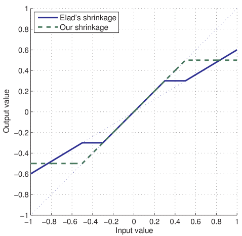
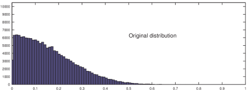
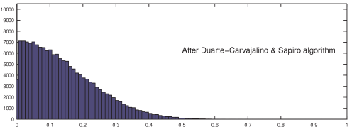
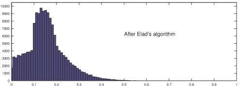
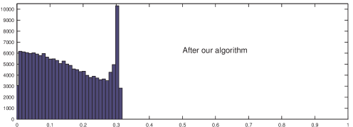
Our method does not produce large off-diagonal elements, in fact, it succeeds to remove all elements that are larger than the given threshold $t$, provided that the target was not too aggressive. Effect of applying both algorithm to the distribution of the magnitude of the off-diagonal entries is demonstrated in Figure 1.5. In this experiment we used a random dictionary $D$ of size $200\times 400$. Its entries we randomly drawn from a normal distribution with zero mean and unity variance. Number of the projections were set to 30, i.e., the size of the projection matrix was $30\times 200$. Effective threshold we used was $26\%$ for the Elad’s algorithm and $0.26$ for our method. The parameter $\gamma$ was set to 0.6 in the Elad’s algorithm.

(a) Histogram of the absolute values of the off-diagonal entries of the Gram matrix $G$ before optimization.

(b) Duarte-Carvajalino & Sapiro’s method

(c) Elad’s method

(d) Our method

Figure 1.5: Histogram of the absolute values of the off-diagonal entries of the Gram matrix $G$ before the optimization and afterwards.

After the optimization, the projection matrix $P$ is both cases does not reveal any specific structure, as we can see in Figure (1.6)

(a) Original

(b) After Duarte-Carvajalino & Sapiro’s method

(c) After Elad’s method

(d) After our method

Figure 1.6: Projection matrix after optimization (a subset of 100 columns).

(a) Initial random projection matrix $P$

(b) After Duarte-Carvajalino & Sapiro’s method

(c) After Elad’s method

(d) After our method

Figure 1.7: Histogram of the values of the projection matrix $P$ before the optimization and afterwards.

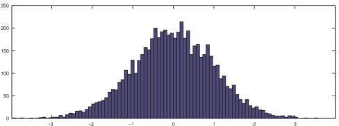
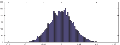
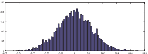
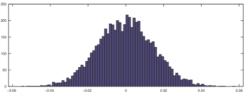
It is also interesting to look at the distribution of the values in the projection matrix before the optimization and afterwards. It seems that the values are still drawn form the Gaussian distribution with zero mean, but the variance is much lower. Our experiments indicate that this is a typical result, that does not depend on the initial guess.

If we consider the final distribution of the off-diagonal entries of the Gram matrix we will find out that it is quite different, as is evident from Figure 1.5. The correlation between the optimized projections matrix $P$ is yet to be theoretically analyzed, therefore, to evaluate the performance of the compressed sensing with and without the optimized projections we performed the following tests:

Stage 1:

Generate data: choose a dictionary $D\in\mathbb{R}^{n\times k}$ and synthesize $N$ test signals $\{x_{i}\}_{i=1}^{N}$ by generating $N$ sparse vectors $\{\theta_{i}\}_{i=1}^{N}$ of length $k$ each, and computing $x_{i}=D\theta_{i}$ for all $i$. All representations $\{\theta_{i}\}$ are built with the same low cardinality $\|c_{i}\|=S$.

Stage 2:

Random projections: for a chosen number of projections $m$ generate a random projection matrix $P\in\mathbb{R}^{m\times n}$ and apply it to the signals to obtain $y_{i}=Px_{i}$. Compute the effective dictionary $\hat{D}=PD$.

Stage 3:

Performance tests: apply the BP and OMP to reconstruct the signals by approximate the solution of

$$\hat{\theta}_{i}=\arg\min_{\theta}\|\theta\|_{0}\mbox{ s.t. }y_{i}=\hat{D}\theta_{i}.$$

The result obtained by the pursuit algorithms is compared against the true solution by evaluating the error $\|\hat{\theta}_{i}-\theta_{i}\|$. Errors above some threshold are considered as a reconstruction failure.

Stage 4:

Optimized projections: the evaluations above are repeated for the projection matrix as returned by the optimization algorithms.

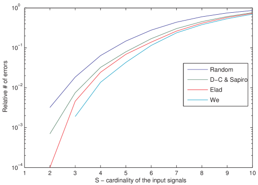
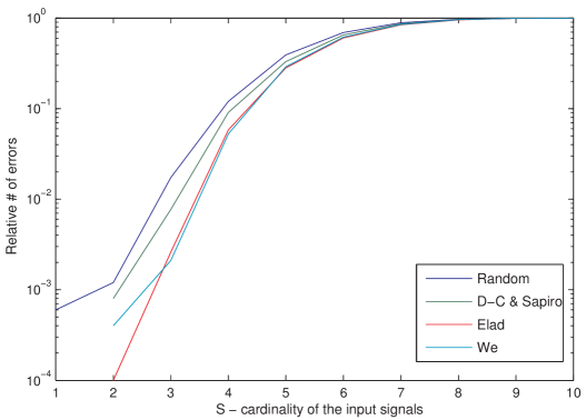
We have followed the above stages to evaluate how the influence of the projection matrix optimization varies along with the cardinality of the true solution. In our experiment we used a random dictionary of size $200\times 400$, i.e., $n=200$, $k=400$. For different of $S$ ($S=1,2,\ldots,10$) we generated $N=10000$ sparse vectors of length $k=400$ with $S$ non-zero values in each. The locations of the non-zero components were chosen at random and populated with i.i.d. zero-mean and unit variance Gaussian values. These sparse vectors were used to create the example signals that were used in the evaluation of the CS performance. The results for the OMP and BP are depicted in Figures 1.8 and 1.9 respectively.

Figure 1.8: CS reconstruction relative errors as a function of the signals’ cardinality $S$. Using OMP method.

Figure 1.9: CS reconstruction relative errors as a function of the signals’ cardinality $S$. Using BP method.

1.4 Simultaneous optimization of the projection matrix and the dictionary

The idea of designing an optimal projection matrix can be taken further if we allow the dictionary $D$ to be changed as well. Let us recall the K-SVD algorithm that is is used for dictionary training. Given an $n\times p$ matrix $X=[x_{1},x_{2},\ldots,x_{p}]$ of $p$ training images of length $n$ pixels each, used to train on overcomplete dictionary $D$ of size $n\times k$, with $p\gg k$ and $k>n$. The objective of the K-SVD algorithm is to solve, for a given sparsity level,

$$\min_{D,\Theta}\|X-D\Theta\|_{F}^{2}\mbox{ s.t. }\|\theta_{i}\|_{0}\leq S,$$ (1.11)

where $\Theta=[\theta_{1},\theta_{2},\ldots,\theta_{p}]$, and $\theta_{i}$ is the sparse vector of coefficients representing the $i$-th image in terms of columns of the dictionary $D=[d_{1},d_{2},\ldots,d_{k}]$. K-SVD is an iterative algorithm that progressively improves the functional in Equation (1.11) as described next. First, the algorithm freezes the current dictionary $D$ and solves for the coefficients’ matrix $\Theta$ using one of the pursuit algorithms. Next, it assumes that the matrises $\Theta$ and $D$ are fixed except for one column of $D$: $d_{j}$. Finding the best $d_{j}$ is done by re-writing the functional in Equation (1.11) as follows

$$\left\|X-D\Theta\right\|_{F}^{2}=\left\|\left(X-\sum_{i\not=j}d_{i}\theta_{T}^{j}\right)-d_{j}\theta_{T}^{j}\right\|_{F}^{2}=\left\|E_{j}-d_{j}\theta_{T}^{j}\right\|_{F}^{2},$$ (1.12)

where $\theta_{T}^{j}$ denotes the $j$-th row of $\Theta$. It is tempting to use the SVD to solve for new $d_{j}$ and $\theta_{T}^{j}$, however, that will lead to a dense $\theta_{T}^{j}$ which is absolutely undesirable. The K-SVD algorithm overcomes this difficulty by using a small subset of columns of $X$ that use the atom $d_{j}$ in their representation. Consequently, the only updated entries of $\theta_{T}^{j}$ are those that are non-zero at the moment. Hence, the algorithm does not increase the density of the coefficients matrix $\Theta.$ After running over all columns of $D$ the algorithm returns to the first step and cycles until convergence, or maximum number of iterations. There exists experimental evidence that the K-SVD algorithm is sensitive to the initial guess, however, this question is not addressed here.

The Coupled-KSVD algorithm suggested by Duarte-Carvajalino and Sapiro extends the KSVD for simultaneous training of the projection matrix $P$ and dictionary $D$ with images available from a dataset. They define the following objective function

$$\min_{P,D,\Theta}\lambda\left\|X-D\Theta\right\|_{F}^{2}+\left\|Y-PD\Theta\right\|_{F}^{2}\mbox{ s.t. }\|\theta_{i}\|_{0}\leq S,$$ (1.13)

where the scalar $\lambda\in[0,1]$ controls the relative weight of the two terms and $Y$ are linear samples given by

$$Y=PX+N,$$ (1.14)

where $N$ represents an additive noise introduced by the sensing system. Let us denote

$$Z=\left(\begin{array}[]{c}\begin{matrix}\lambda X\\ Y\end{matrix}\end{array}\right),\,W=\left(\begin{matrix}\lambda I\\ P\end{matrix}\right).$$ (1.15)

Then, Equation (1.13) can be re-written as,

$$\min_{P,D,\Theta}\left\|Z-\tilde{D}\Theta\right\|\mbox{ s.t. }\left\|\theta_{i}\right\|_{0}\leq S,$$

where $\tilde{D}=WD$. Now, in exactly the same manner as we did in the K-SVD we run over all columns of $\tilde{D}$ one by one and find simultaneous solution for $\tilde{d}_{j}$ and $\theta_{T}^{j}$. Then, we substitute back

$$\tilde{d}_{j}=\left(\begin{matrix}\lambda I\\ P\end{matrix}\right)d_{j}.$$ (1.16)

At this point, we have $m+n$ equations and $n$ unknowns. The solution is obtained by solving the overdetermined system in the sense of the least squares, thus the unknown column $d_{j}$ can be found by

$$d_{j}=\left(\lambda^{2}I+P^{T}P\right)^{-1}\left(\begin{matrix}\lambda I&P^{T}\end{matrix}\right)\tilde{d}_{j}.$$ (1.17)

Finally, the norm of $d_{j}$ is adjusted to unity (of course, this step must be accompanied by adjusting the row $\theta_{T}^{j}$) to keep the product $\tilde{d}_{j}\theta_{T}^{j}$ without any change), i.e.,

$$\theta_{T}^{j}=\theta_{T}^{j}\|d_{j}\|_{2},\quad d_{j}=d_{j}/\|d_{j}\|_{2}$$ (1.18)

After we finished the update of the dictionary $D$ and the coefficient matrix $\Theta$, assuming fixed $P$, we can update the projection matrix, with the methods described in the previous section, i.e., learning the projection matrix from the just updated dictionary $D$. Then, we repeat the algorithm until convergence. Hence, the whole algorithm is formalized in Algorithm 1.4.

• Objective: Minimize $\lambda\left\|X-D\Theta\right\|_{F}^{2}+\left\|Y-PD\Theta\right\|_{F}^{2}\mbox{ s.t. }\|\theta_{i}\|_{0}\leq S$ with respect to $P$,$D$, and $\Theta$.

  Input: Use the following parameters:

  • $X$,$Y$ - the training data and its projections

  • $\lambda$ - weight of the first term ($0\leq\lambda\leq 1$)

  Initialization:

  1. set initial dictionary $D_{0}\in\mathbb{R}^{p\times n}$ to an arbitrary random matrix

  Loop: Set $q=0$ (iteration counter) and repeat until convergence:

  1. For fixed $D_{q}$ compute $P_{q}$ using an algorithm from the previous section.

  2. For fixed $D_{q}$ and $P_{q}$ compute $\Theta_{q}$ using a pursuit algorithm, e.g., OMP.

  3. Using update $P_{q}$, $D_{q}$, and $\Theta_{q}$ by the K-SVD, as described in Equations 1.16,1.17, and 1.18.

  EndLoop

Algorithm 1.4 Coupled KSVD.

Experimental results of this approach are available in the original paper.

1.5 Conclusions

We presented several algorithms for optimization of the projection matrix used in the Compressed Sensing. Experimental results indicate that our method performs better than the the other two. Simultaneous method of optimization of the projection matrix and the sparsifying dictionary as suggested by Duarte-Carvajalino and Sapiro was presented in a descriptive manner without experimental results.

References

- [1] M. Aharon, M. Elad, and A. Bruckstein. K-SVD: an algorithm for designing overcomplete dictionaries for sparse representation. IEEE Transactions on signal processing, 54(11):4311, 2006.
- [2] J. M. Duarte-Carvajalino and G. Sapiro. IMA preprint series# 2211.
- [3] M. Elad. Optimized projections for compressed sensing. Signal Processing, IEEE Transactions on, 55(12):5695–5702, 2007.
- [4] J. A. Tropp, I. S. Dhillon, R. W. Heath, and T. Strohmer. Designing structured tight frames via an alternating projection method. IEEE Transactions on information theory, 51(1):188–209, 2005.