Actively stressed marginal networks

Abstract

We study the effects of motor-generated stresses in disordered three dimensional fiber networks using a combination of a mean-field, effective medium theory, scaling analysis and a computational model. We find that motor activity controls the elasticity in an anomalous fashion close to the point of marginal stability by coupling to critical network fluctuations. We also show that motor stresses can stabilize initially floppy networks, extending the range of critical behavior to a broad regime of network connectivities below the marginal point. Away from this regime, or at high stress, motors give rise to a linear increase in stiffness with stress. Finally, we demonstrate that our results are captured by a simple, constitutive scaling relation highlighting the important role of non-affine strain fluctuations as a susceptibility to motor stress.

The mechanical properties of cells are regulated in part by internal stresses generated actively by molecular motors in the cytoskeletal filamentous actin network Howard (2001). On a larger scale, collective motor activity allows the cell to contract the surrounding extracellular matrix, consisting also of biopolymer networks. Experiments show that such active contractility dramatically affects network elasticity, both in reconstituted intracellular F-actin networks with myosin motors Mizuno et al. (2007); Bendix et al. (2008); Koenderink et al. (2009); Gordon et al. (2012) and in extracellular matrices with contractile cells Lam et al. (2011). The dynamics and elasticity of active biopolymer networks have been studied theoretically using long-wavelength hydrodynamic approaches as well as affine models MacKintosh and Levine (2008); Liverpool et al. (2009); Shokef and Safran (2012). These approaches, however, fail to describe highly disordered networks. There is also experimental evidence that cytoskeletal networks may be unstable or only marginally stable in the absence of motor activity Cai et al. (2010). In such cases, networks are expected to be governed by highly nonuniform, soft or floppy modes of deformation that may lead to a fundamental breakdown or failure of continuum elasticity Broedersz et al. (2011). Importantly, motor-induced contractile stresses can be expected to couple to these soft modes, giving rise to a nonlinear elastic response that is distinct from the nonlinearities arising from single fiber elasticity that have been considered in previous models. Moreover, such a coupling to local soft modes of the network may call into question the equivalence of internal (motor) and external stress, a tacit assumption in the analysis of recent in vitro experiments Mizuno et al. (2007); Koenderink et al. (2009).

Here, we introduce a simple model to study the effects of motor generated stresses in disordered fiber networks. Networks are formed by crosslinked straight fibers with linear stretching and bending elasticity. These fibers are organized on a face centered cubic (FCC) lattice in which a certain fraction of the the bonds can randomly be removed. Motor activity is introduced by contractile force dipoles acting between neighboring network nodes. We find that motors can stabilize the elastic response of otherwise floppy, unstable networks. The motor stress also controls the mechanics of stable networks above a characteristic threshold, in the vicinity of which the network exhibits critical strain fluctuations. We develop a quantitative effective medium theory to describe the elastic response of these systems. Interestingly, the network’s stiffness is controlled by a coupling of the motor induced stresses to the strain fluctuations. This coupling gives rise to anomalous regimes at the stability thresholds, at which network criticality is reflected in both divergent strain fluctuations and anomalous dependences of the network mechanics on stress. In these critical regimes, the shear modulus depends nonlinearly on both motor stress and single filament elasticity Lam et al. (2011); Ehrlicher and Hartwig (2011); Broedersz and MacKintosh (2011); Chen and Shenoy (2011). Interestingly, this dependence on internal motor stress differs qualitatively from that of an applied external stress.

A key parameter that characterizes fiber networks is the mean coordination number, $z$. Although the network is connected above a threshold $z=z_{\rm cond}\simeq 2$, it only becomes rigid above a higher rigidity threshold $z_{b}\simeq 3.4$. This threshold is due to the bending rigidity of the individual fibers and it lies below the central-force (CF) rigidity threshold, $z_{\rm cf}\simeq 6$, for a spring-only network. In general, when some fraction of the bonds are under stress, additional constraints are introduced Huisman and Lubensky (2011). More formally, these constraints appear as scalar terms in the Hamiltonian Alexander (1998). These additional stress-constraints may shift the various rigidity thresholds in the system. In random spring networks, for example, this can be realized by applying finite network deformations; this has been studied in spring networks Tang and Thorpe (1988); Wyart et al. (2008); Sheinman et al. (2012) where the actual rigidity threshold shifts continuously to lower values with the applied external strain. Under such external deformations, the internal stress is free to adopt the most favorable distribution. By contrast however, motors impose a fixed distribution of internal stress, which may lead to a qualitatively different network mechanics.

To provide insight into the elasticity of fibrous networks with contractile internal stresses, we use a model of fibers organized on a FCC lattice. By removing lattice-bonds with a probability $1-p$, we tune the average coordination number, $z=\mathcal{Z}p$, where $\mathcal{Z}=12$ for the undiluted lattice. Motors are introduced as contractile force dipoles and are inserted randomly with a probability $q$. The fibers are modeled as linear elastic beams with a stretching modulus $\mu$ and bending rigidity $\kappa$. Using units in which $\ell_{0}=\mu=1$, the total energy can be written as

$$H =\frac{1}{2}\sum\limits_{\langle ij\rangle}P_{ij}\left(\lvert\mathbf{r}_{ij}\rvert-1\right)^{2}$$

$$+\frac{\kappa}{2}\sum\limits_{\langle ijk\rangle}P_{ij}P_{jk}\left(\frac{\mathbf{r}_{ij}\times\mathbf{r}_{jk}}{\lvert\mathbf{r}_{ij}\rvert\lvert\mathbf{r}_{jk}\rvert}\right)^{2}$$

$$+f\sum\limits_{\langle ij\rangle}Q_{ij}\lvert\mathbf{r}_{ij}\rvert$$ (1)

where, $\mathbf{r}_{ij}=\mathbf{r}_{i}-\mathbf{r}_{j}$ and $\mathbf{r}_{i}$ denotes the position of $i$’th node and $P_{ij}=1$ for present bonds or $P_{ij}=0$ for removed bonds. The first sum extends over neighboring pairs of vertices. The crosslinks themselves do not contribute a torsional stiffness and, thus, the second sum only extends over coaxial nearest neighbor bonds on the same fiber. The last term represents the work performed by the motors, where $Q_{ij}=1$ if a motor acts between nodes $i$ and $j$ and $Q_{ij}=0$ otherwise.

To develop a mean-field, effective medium theory (EMT) that captures the disordered nature of this model—including internal stresses—we extend the theory for the linear mechanical response of disordered spring networks  Feng et al. (1985); Schwartz et al. (1985); Mao et al. (2010). In our EMT approach we ignore the bending contribution ($\kappa=0$), allowing us to circumvent the difficulties involved in an EMT with three-point bending interactions Broedersz et al. (2011); Das et al. (2007); Mao et al. (2011). Our EMT is based on a mapping between the disordered and an ordered network with an effective elastic constant, yet with the same underlying lattice geometry and under the same internal stress as the original disordered system. The effective elastic constant, $\widetilde{\mu}\left(\sigma_{M}\right)$, is determined by a self-consistency condition; the local distortion in the effective medium induced by replacing a bond, selected randomly from the disordered system, should vanish on average. For a general disordered network this procedure yields an implicit expression for the effective stretch modulus (see Appendix)

$$\int_{0}^{\infty}\frac{\mu_{ij}-\widetilde{\mu}\left(\sigma_{M}\right)}{\mu_{EM}+\mu_{ij}-\widetilde{\mu}\left(\sigma_{M}\right)}\mathcal{P}\left(\mu_{ij}\right)d\mu_{ij}=0,$$ (2)

where $\mu_{EM}$ is the displacement of a bond in the unperturbed effective medium due to a unit force acting along the bond, $\mu_{ij}$ is the stretching modulus between nodes $i$ and $j$ and $\mathcal{P}\left(\mu_{ij}\right)$ is the probability density of the moduli in the disordered system. For the case of a diluted lattice considered here, $\mathcal{P}\left(\mu_{ij}\right)=p\delta\left(\mu_{ij}-1\right)+\left(1-p\right)\delta\left(\mu_{ij}\right)$, we find the EMT shear modulus

$$G_{EM}=\frac{5\sqrt{2}}{72}\widetilde{\mu}\left(\sigma_{M}\right)+\frac{5}{6}\sigma_{M},$$ (3)

where, within the EMT, $\sigma_{M}=\sqrt{8}qf$.

While the full expression for $\widetilde{\mu}\left(\sigma_{M}\right)$ is long (see Appendix), the scaling predictions of the EMT are simple. Even below the central-force isostatic point, $z_{\rm cf}$, motor activity induces a finite shear modulus. Far from $z_{\rm cf}$, $G\sim G_{0}+\sigma_{M}$, where $G_{0}$ is the shear modulus of the unstressed network. By contrast, close to $z_{\rm cf}$ there is an anomalous scaling regime $G\sim\sigma_{M}^{1/2}\mu^{1/2}$.

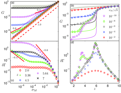
Figure 1: (a) Shear modulus is shown vs. motor stress for different values of the coordination number $z$. Markers represent the numerical data (see legend in (c)). Thin, solid lines represent the results of the EMT for the same values of $z$ while upper lines correspond to higher values of $z$. Lines with numbers represent the corresponding slopes and thick grey area contains the affine predictions for all presented coordination numbers. (b) $G$ is shown vs. $z$ for different values of $\sigma_{M}$. Markers represent numerical data (see legend). Thin, solid lines represent the results of the EMT for the same values of $\sigma_{M}$ while upper lines correspond to higher values of $\sigma_{M}$. Thick grey area contains the affine predictions for all presented values of $\sigma_{M}$. (c) The differential non-affinity parameter is presented vs. motor stress for different values of $z$ (see legend). (d) $\delta\Gamma$ is presented vs. $z$ for different values of $\sigma_{M}$ (see legend in (b)). For all data sets $\kappa=10^{-5}$.

To test the implications of the EMT, we perform simulations of fiber networks with finite bending rigidities. The shear modulus, $G$, is determined numerically by applying a shear strain along the $111$-plane using Lees-Edwards periodic boundary conditions and energy minimizations are performed by a conjugate gradient algorithm Press et al. (1992). First, we consider the high motor density limit $q\simeq 1$. The EMT prediction is in good quantitative agreement with the numerical results over a broad range of network connectivity and motor stress, as shown in Fig. 1 a,b. Since we neglected the contribution of fiber bending energies in the EMT, it fails in the regime where $G$ is governed by $\kappa$. In addition, in the vicinity of $z_{cf}$ for $\sigma_{M}\gg\kappa$, we find a mixed regime, $G\sim\mu^{1-y^{\prime}}\sigma_{M}^{y^{\prime}}$, where $y^{\prime}=0.4$, whereas in the EMT $y^{\prime}=0.5$ (Fig. 2). This mixed regime is similar in nature to the $\kappa$-$\mu$ coupled mechanical regime around $z_{cf}$ in unstressed fibrous networks Broedersz et al. (2011). More generally, such coupled regimes arise in the vicinity of a stability threshold, when there are additional interactions or fields that stabilize the network below the threshold Wyart et al. (2008). Thus, in this model the motor stress acts as an external field. In fact, as may be expected, another anomalous regime is observed in the simulations at the bending rigidity threshold, $G\sim\kappa^{1-y}\sigma_{M}^{y}$, with $y=0.6$ (Figs. 1 and 2).

We gain additional physical insight into the elastic properties of active networks with a scaling argument we estimate the amount of work that is performed by the motors when the system is sheared. The characteristic deformation of a single bond in such a network will be such that it avoids energetically costly stretching contributions. Such deformations are oriented perpendicularly to the direction of the bond: the nonaffine contribution to this deformation can be estimated by $\delta u_{\perp}\sim\gamma\sqrt{\delta\Gamma}$, where the differential nonaffinity parameter is defined as,

$$\delta\Gamma=\frac{1}{\gamma^{2}}\left\langle\left(\delta\textbf{u}_{k}-\delta\textbf{u}_{k}^{\rm aff}\right)^{2}\right\rangle_{k}.$$ (4)

Here $\delta\textbf{u}_{k}$ is the displacement of node $k$ under an infinitesimal external shear $\gamma$, $\delta\textbf{u}_{k}^{\rm aff}$ is the affine prediction and the average is taken over all network nodes. Interestingly however, this is not the only relevant contribution to the deformation of the bond. The component of the affine deformation perpendicular to the bond does not contribute to bond-stretching energies to harmonic order and, thus, is not avoided. Importantly however, this deformation does contribute to the motor work. Therefore, the total work performed by the internal stress resulting from such deformations scales as $\delta W\sim\sigma_{M}\gamma^{2}\delta\Gamma+\sigma_{M}\gamma^{2}$, implying the following relationship for the shear modulus,

$$G\sim G_{0}+\sigma_{M}\delta\Gamma+\sigma_{M}.$$ (5)

The non affinity parameter, $\delta\Gamma(\sigma_{M},z,\kappa)$, depends on the system’s parameters as shown in Fig. 1c,d. To confirm the prediction of Eq. (5) we plot $G-G_{0}-\frac{5}{6}\sigma_{M}$ vs. $\sigma_{M}\delta\Gamma$ and find that all data collapses on to the same curve with a linear dependence, as shown in Fig. 3(a). Interestingly, the scaling prediction in Eq. (5) suggests that $\delta\Gamma$ can be interpreted as a susceptibility of the shear modulus to the internally generated stress. Moreover, $\delta\Gamma$ shows a strong increase close to both rigidity thresholds (Fig. 1 d), implying a large susceptibility to $\sigma_{M}$ when the system is marginally stable. However, at these stability thresholds $\delta\Gamma$ acquires a strong dependence on $\sigma_{M}$. This can be understood by considering $\sigma_{M}$ as an external field that restores rigidity and suppresses the divergence of the strain fluctuations $\delta\Gamma\sim\left|\Delta z\right|^{-\lambda}$ (for $\sigma_{M}=0$); this implies a dependence of the form $\delta\Gamma(z_{b})\sim(\kappa/\sigma_{M})^{-y}$ and $\delta\Gamma(z_{\rm cf})\sim(\mu/\sigma_{M})^{-y^{\prime}}$ and, taken together with Eq. (5), explains the origins of the anomalous regimes, where

$$G(z_{b})\sim\kappa^{y}\sigma_{M}^{1-y},\ \ \ G(z_{\rm cf})\sim\mu^{y^{\prime}}\sigma_{M}^{1-y^{\prime}}.$$ (6)

We verified the internal consistency by determining the exponents $y$ and $y^{\prime}$ at the two stability thresholds from both the scaling of $G$ and $\delta\Gamma$ with $\sigma_{M}$, as shown in Fig. 2.

The schematic phase diagram for the high-motor density limit is shown in Fig. 3(b). Away from the stability thresholds the shear modulus scales linearly with the active stress. This is in contrast with the stiffening behavior of externally deformed networks, for which the dependence of the differential elastic modulus goes as the square root of the external stress  Wyart et al. (2008); Sheinman et al. (2012). Thus, there is not necessarily a quantitative correspondence between internally and externally stressed networks, in contrast to suggestions in prior work Koenderink et al. (2009).

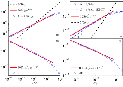
Figure 2: Demonstration of the anomalous regimes. (a) Shear modulus separated to the linear part, $5/6\sigma_{M}$ (dashed line), and the rest, $G-5/6\sigma_{M}$ (circles) is shown for $z=3.35$ (close to the bending rigidity percolation point, $z_{b}\simeq 3.36$) and $\kappa=10^{-2}$. In the small stress limit the $G-5/6\sigma_{M}$ part is found to scale as $\sigma_{M}^{1-y}$ with $y\simeq 0.6$ (solid line). (b) The same analysis as in (a) is shown for $z=5.9$ (close to the central-force rigidity percolation point, $z_{\rm cf}\simeq 5.64$) and $\kappa=0$. In the small stress limit the $G-5/6\sigma_{M}$ part is found to scale as $\sigma_{M}^{1-y^{\prime}}$ with $y^{\prime}\simeq 0.4$ (solid line), in contrast to the mean-field prediction (indicated by the dashed-dotted line) that scales as $\sqrt{\sigma_{M}}$ in the small stress limit. (c) The value of $\delta\Gamma$ (circles) is presented for the same set of parameters as in (a). In the small stress limit it scales as $\sigma_{M}^{-y}$ (solid line). (d) The value of $\delta\Gamma$ (circles) is presented for the same set of parameters as in (b). In the small stress limit it scales as $\sigma_{M}^{-y^{\prime}}$ (solid line).

Finally, we explore the role of inhomogeneity in the distribution of active motors, which shows that critical behavior is not limited to the critical points associated with rigidity percolation. We model inhomogeneous motors by considering the range $q<1$ for different values of $z$ well below the rigidity percolation point, $z<z_{b}$. In this case the motors only induce a macroscopic stress when the motor density exceeds a $z$-dependent threshold, $q_{c}\left(z\right)$, as shown in Fig. 4(b). Concurrent with the development of a macroscopic stress, the network acquires a finite shear rigidity. Near the threshold $q_{c}$, the motor-induced stress falls significantly below the mean-field prediction ($\sigma_{M}=\sqrt{8}qf$) and depends non-linearly on $q$. Interestingly, in this regime ($\sigma_{M}\ll\sqrt{8}q_{c}f$) the nonaffine fluctuations become large (see Fig. 4(d)), diverging with motor stress with an exponent close to $-0.2$, as shown in Fig. 4(c). Such a divergence, taken together with Eq. (5) implies an anomalous, sub-linear scaling of the shear modulus with the motors stress with the exponent $0.8$. Indeed, as shown in Fig. 4(a), the stiffening of the shear modulus clearly deviates from the mean-field predictions and scales sublinearly with the motor stress with an $0.8$ exponent, consistent with Eq. (5), even when the mean coordination number of the network is well below the rigidity percolation point. Thus, criticality in the form of a divergent susceptibility is characteristic of floppy systems below the rigidity percolation point.

This work demonstrates that motor activity controls the elastic properties of disordered networks by coupling to the differential non-affine fluctuations in the deformation field. This coupling makes elastic deformations more affine and stabilizes the network. Far from the elastic critical points this coupling leads to linear stiffening as a function of the motors stress, as has been observed in several studies of prestressed elastic networks Budiansky and Kimmel (1987); Stamenovic and Coughlin (2000). However, close to the elastic critical points, where the non-affine fluctuations diverge, this coupling leads to anomalous regimes, where the shear modulus scales sub-linearly with the motors stress. Similar stress-stiffening of floppy networks below marginal stability is also found beyond a threshold in the motor density, indicating that a surprising generality of critical fluctuations and divergent susceptibility for systems below the usual rigidity percolation point.

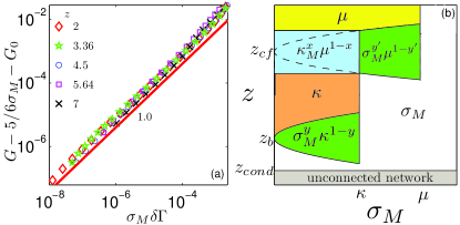
Figure 3: (a) Collapse on the data presented on Fig. 1(a) based on Eq. (5). Red line represents linear dependence. (b) The schematic phase diagram for the rigidity of random spring networks under an internal stress $\sigma_{M}$.

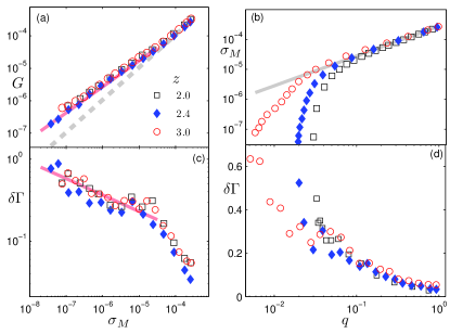
Figure 4: The role of inhomogeneity in the motor distribution for different values of $z$ (see legend on panel (a) for every plot in this figure). (a) Shear modulus is presented vs. the normal stress induced by the motors. Solid line represents the power law of $0.8$ while the dashed line contain the mean-filed predictions. (b) The normal stress vs. the motor probability occupation. Solid line represents the mean-field prediction, $\sigma_{M}=\sqrt{8}qf$. (c) The differential non-affine fluctuations measure for the same data as in (a) is presented vs. $\sigma_{M}$. The solid line represents the power law of $-0.2$. (d) $\delta\Gamma$ vs. $q$. For all the data in this figure $f=10^{-4}$ and $\kappa=10^{-5}$.

Appendix A Mean-field approach

The nonlinear EM approach developed here is based on a scheme to construct a mapping from the internally stressed lattice network with disordered spring constant, $\mu_{ij}$, with probability density $P\left(\mu_{ij}\right)$, onto a perfect lattice system with uniform bond stiffness with the same stress, $\sigma_{M}$. The stress of the network appears due to motors’ force $f$ that acts between each pair of neighboring nodes of the network. This mapping is realized by an effective uniform central force interaction, $\mu_{ij}\rightarrow\widetilde{\mu}$. The effective parameter, $\widetilde{\mu}$$\left(\sigma_{M}\right)$, is determined by a self-consistency requirement: replacing a random bond in the uniform EM under stress with a bond drawn from the original probability density, $P\left(\mu_{ij}\right)$, results in a local fluctuation in the deformation field, which vanishes when averaged. In addition, we assume that the fluctuations of the deformations are small compared to the distance between crosslinks. This approach leads to an integral equation, representing a disorder average (Eq. (21)), from which the effective parameter $\widetilde{\mu}(\sigma_{M})$ can be determined. In the following we ignore the contribution of the bending stiffness of the network filaments. Due to this assumption the presented mean-field approach fails in the regime where the elasticity of the network is dominated by the bending stiffness.

A.1 Effective medium theory

We apply the EM theory method to a network subjected to a uniform internal compression resulting in a macroscopic isotropic stress $\sigma_{M}$. Similarly to Ref. Feng et al. (1985), we calculate the effective spring constant using the self-consistency requirement.

The position of a crosslink (network’s node) $i$ is given by $\mathbf{R}_{i}=\mathbf{R}_{i}^{0}+\mathbf{u}_{i}$, where $\mathbf{R}_{i}^{0}$ is the position in the unstressed configuration and $\mathbf{u}_{i}$ is the displacement field. In order to calculate the elastic constant we apply an infinitesimal external expansional/comressional strain $\epsilon$ to the network. The affine displacement due to the applied strain is given by $\mathbf{u}_{i}^{\rm aff}-\mathbf{u}_{j}^{\rm aff}=\epsilon\mathbf{r}_{ij}$, where $\mathbf{r}_{ij}$ is the vector from $\mathbf{R}^{0}_{i}$ to $\mathbf{R}^{0}_{j}$ in the undeformed reference state. Here we allow for non-affine displacements

$$\mathbf{v}_{i}\equiv\mathbf{u}_{i}-\mathbf{u}_{i}^{\rm aff},$$ (7)

The Hamiltonian of the network is given by

$$H=\frac{1}{2}\sum\limits_{\langle ij\rangle}\mu_{ij}\left(\lvert\mathbf{R}_{ij}\rvert-1\right)^{2}+f\sum\limits_{\langle ij\rangle}\lvert\mathbf{R}_{ij}\rvert,$$ (8)

where $\mathbf{R}_{ij}=\mathbf{R}_{j}-\mathbf{R}_{i}$ and the sums extend over neighboring pairs of vertices. We assume that the resulting non-affine relative displacements of neighbouring nodes $i$ and $j$ are much smaller than the distance between the nodes,

$$\left|\mathbf{v}_{ij}\right|\equiv\left|\mathbf{v}_{i}-\mathbf{v}_{j}\right|\ll\left|\mathbf{R}_{i}^{0}-\mathbf{R}^{0}_{j}\right|=1.$$ (9)

Thus, we can expand the Hamiltonian around the affine strain configuration (small $v_{ij}$). Up to second order in $v_{ij}$ and first order in $\epsilon$ we arrive at Tang and Thorpe (1988); Alexander (1998)

$$H=\underset{\left\langle ij\right\rangle}{\sum}f+\left(f+\epsilon\mu_{ij}\right)\mathbf{v}_{ij}\cdot\mathbf{r}_{ij}+\frac{1}{2}\left(\mu_{ij}-f\right)\left(\mathbf{v}_{ij}\cdot\mathbf{r}_{ij}\right)^{2}+\frac{1}{2}f\mathbf{v}_{ij}^{2}.$$ (10)

The first term represents the expansion/compression energy of the affine response, while the other terms correspond to the energy difference due to the non-affine deformation of the stretched/compressed bonds.

The expansion of the whole network corresponds to the global constraint

$$\underset{\left\langle ij\right\rangle}{\sum}\mathbf{v}_{ij}=0.$$ (11)

To investigate the elastic behavior of the model in Eq. (10), we set up an effective medium theory. In the EM approach, we mimic the disordered system by the regular one with an effective parameter, i.e. $\mu_{ij}\rightarrow\widetilde{\mu}$ and the same stress $\sigma_{M}$. In other words, the EM network may be globally expanded by applying the force that assures mechanical equilibrium for the affine, $\mathbf{v}_{ij}=0$, configuration. Thus, the EM system has the Hamiltonian, given by

$$H_{EM}=\underset{\left\langle ij\right\rangle}{\sum}f+\left(f+\epsilon\widetilde{\mu}\right)\mathbf{v}_{ij}\cdot\mathbf{r}_{ij}+\frac{1}{2}\left(\widetilde{\mu}-f\right)\left(\mathbf{v}_{ij}\cdot\mathbf{r}_{ij}\right)^{2}+\frac{1}{2}f\mathbf{v}_{ij}^{2}+\mathbf{\Lambda}_{ij}\cdot\mathbf{v}_{ij}$$ (12)

where $\mathbf{\Lambda}_{ij}=-\left(f+\epsilon\widetilde{\mu}\right)\mathbf{r}_{ij}$. To calculate the effective parameter $\widetilde{\mu}$ we demand self-consistency of the EM Feng et al. (1985). The self-consistency requirement in this context can be formulated as follows: the non-affine displacement induced by the replacement of a single bond in the EM vanishes on average,

$$\left\langle\mathbf{v}_{nm}\right\rangle=0.$$ (13)

Here, the average is taken over the distribution of the $nm$ bond in the original disordered system, i.e. according to the probability density $P\left(\mu_{nm}\right)$. To calculate the displacement $\mathbf{v}_{nm}$ after the replacement we solve the perturbed EM Hamiltonian that is given by

$$H_{EM}+\frac{1}{2}\left(\mu_{nm}-\widetilde{\mu}\right)\left(\mathbf{v}_{nm}\cdot\mathbf{r}_{nm}\right)^{2}+\mathbf{v}_{nm}\cdot\mathbf{r}_{nm}\epsilon\left(\mu_{nm}-\widetilde{\mu}\right)$$ (14)

In the configuration that minimizes the energy, the displacement of the $nm$ bond is given by

$$\mathbf{v}_{nm}=\frac{\mathbf{r}_{nm}\epsilon\left(\mu_{nm}-\widetilde{\mu}\right)}{\mu_{EM}+\mu_{nm}-\widetilde{\mu}},$$ (15)

where $\mu_{EM}$ is the displacement of the $nm$ bond in the unperturbed EM network due to a unit force acting along the $nm$ bond.

A.1.1 The calculation of $\widetilde{\mu}_{EM}$

In this Section we calculate $\mu_{EM}$—the displacement of the $nm$ bond in the unperturbed EM network due to a unit force $\mathbf{r}_{nm}$ acting on the $nm$ bond.

The dynamical matrix of the unperturbed EM Hamiltonian (12) is given by

$$D_{ij}=\begin{cases}-\left(\widetilde{\mu}-f\right)\mathbf{r}_{ij}\otimes\mathbf{r}_{ij}+f\mathbb{I}&i\neq j\\ \underset{j\neq i}{\sum}\left[\left(\widetilde{\mu}-f\right)\mathbf{r}_{ij}\otimes\mathbf{r}_{ij}+f\mathbb{I}\right]&i=j\end{cases},$$ (16)

where $\mathbb{I}$ is the unit tensor and $\otimes$ is the external product. The Fourier transform of $D$ is given by

$$D\left(\mathbf{k}\right) = \underset{ij}{\sum}D_{ij}e^{i\mathbf{k}\cdot\mathbf{r}_{ij}}=$$ (17)

$$= \underset{\mathbf{r}}{\sum}\left(\left(\widetilde{\mu}-f\right)\mathbf{r}\otimes\mathbf{r}+f\mathbb{I}\right)\left(1-e^{i\mathbf{k}\cdot\mathbf{r}}\right)$$

where $\mathbf{r}$ runs over all unit bond vectors. The unit force acting on the $nm$ bond is given by

$$\mathbf{f}_{i}=\mathbf{r}_{nm}\left(\delta_{i,n}-\delta_{i,m}\right),$$ (18)

so that its Fourier transform is

$$\mathbf{f}\left(\mathbf{k}\right)=\underset{i}{\sum}\mathbf{f}_{i}e^{i\mathbf{k}\cdot\mathbf{R}_{i}}=\mathbf{r}_{nm}\left(1-e^{i\mathbf{k}\cdot\mathbf{r}_{nm}}\right).$$ (19)

Thus the Fourier transform of the displacement field is given by

$$\mathbf{v}\left(\mathbf{k}\right)=-D^{-1}\left(\mathbf{k}\right)\cdot\mathbf{f}\left(\mathbf{k}\right).$$ (20)

The displacement of the $nm$ bond due to the unit force is

$$\mu_{EM}^{-1} =\frac{1}{N}\mathbf{r}_{nm}\cdot\underset{\mathbf{k}}{\sum}\mathbf{v}\left(\mathbf{k}\right)\left(e^{-i\mathbf{k}\cdot\mathbf{r}_{nm}}-1\right)=-\underset{\mathbf{k}}{\sum}\mathbf{r}_{nm}\cdot\mathbf{f}\left(\mathbf{k}\right)D^{-1}\left(\mathbf{k}\right)\left(e^{-i\mathbf{k}\cdot\mathbf{r}_{nm}}-1\right)$$

$$=\widetilde{\mu}^{-1} \frac{2d}{\mathcal{Z}}\left[1-\frac{f}{dN\left(\widetilde{\mu}-f\right)}\underset{\mathbf{k}}{\sum}Tr\left\{\frac{\underset{\mathbf{r}}{\sum}\left(1-e^{i\mathbf{k}\cdot\mathbf{r}}\right)}{\underset{\mathbf{r}}{\sum}\left(\mathbf{r}\otimes\mathbf{r}+\frac{f}{\widetilde{\mu}-f}\mathbb{I}\right)\left(1-e^{i\mathbf{k}\cdot\mathbf{r}}\right)}\right\}\right].$$

For a highly coordinated lattice the sum over $\mathbf{r}$ may be well approximated by the integral over the sphere that includes all the neighbouring crosslinks and, since the sum over $\mathbf{k}$ is dominated by the small $\mathbf{k}\cdot\mathbf{r\ll 1}$ values, $\mu_{EM}$ may be approximated by

$$\mu_{EM}^{-1} \simeq \widetilde{\mu}^{-1}\frac{2d}{\mathcal{Z}}\left[1-\frac{f}{dN\left(\widetilde{\mu}-f\right)}Tr\left\{\frac{\oint\left(\mathbf{k}\cdot\mathbf{r}\right)^{2}d^{d-1}\mathbf{r}}{\oint\left(\mathbf{k}\cdot\mathbf{r}\right)^{2}d^{d-1}\mathbf{r}\left(\mathbf{r}\otimes\mathbf{r}+\frac{f}{\widetilde{\mu}-f}\mathbb{I}\right)}\right\}\right]$$

$$= \widetilde{\mu}^{-1}\frac{2d}{\mathcal{Z}}\left[1-\frac{f}{d\left(\widetilde{\mu}-f\right)}\left(\frac{1}{\frac{3}{2+d}+\frac{f}{\widetilde{\mu}-f}}+\frac{d-1}{\frac{1}{2+d}+\frac{f}{\widetilde{\mu}-f}}\right)\right].$$

A.1.2 An effective elastic constant

Given Eqs. (13,15,A.1.1), the self-consistency Eq. (13) leads to the following equation for the effective parameter

$$\int_{0}^{\infty}\frac{\mu_{ij}-\widetilde{\mu}\left(\sigma_{M}\right)}{\mu_{EM}+\mu_{ij}-\widetilde{\mu}\left(\sigma_{M}\right)}P\left(\mu_{ij}\right)d\mu_{ij}=0.$$ (21)

The approach presented in this section allows one to calculate the elastic parameters of a system with a given topology and elastic constant distribution in the nonlinear elastic regime. Eq. (21) may be solved numerically for any realization of the spring constant probability density, $P\left(\mu_{ij}\right)$. Knowing the effective spring constant, $\widetilde{\mu}$, one obtains all the elastic constants of the network and the relation between the motors’ applying force, $f$ and the global normal network’s stress, $\sigma_{M}$. In the next section we demonstrate the presented method using the particular example of diluted regular networks when Eq. (21) can be solved analytically.

A.2 Diluted regular networks

In this Section we use the mean-field solution presented above using for particular example of bond-diluted regular networks. The probability density for the spring constants for such a network is given by

$$P\left(\mu_{ij}\right)=\frac{z}{\mathcal{Z}}\delta\left(\mu_{ij}-\mu\right)+\left(1-\frac{z}{\mathcal{Z}}\right)\delta\left(\mu_{ij}\right).$$ (22)

Networks of this kind are referred to as diluted spring networks or the central-force elastic percolation model. The linear elastic response of diluted, unstressed lattices has been extensively studied Feng and Sen (1984); Feng et al. (1985). Here we show how these results generalize for internally stressed networks.

In this case the Eq. (21) becomes

$$\frac{\frac{\widetilde{\mu}}{\mu-\widetilde{\mu}}+\frac{2d}{\mathcal{Z}}\left[1-\frac{f}{d\left(\widetilde{\mu}-f\right)}\left(\frac{1}{\frac{3}{2+d}+\frac{f}{\widetilde{\mu}-f}}+\frac{d-1}{\frac{1}{2+d}+\frac{f}{\widetilde{\mu}-f}}\right)\right]}{1-\frac{2d}{\mathcal{Z}}\left[1-\frac{f}{d\left(\widetilde{\mu}-f\right)}\left(\frac{1}{\frac{3}{2+d}+\frac{f}{\widetilde{\mu}-f}}+\frac{d-1}{\frac{1}{2+d}+\frac{f}{\widetilde{\mu}-f}}\right)\right]}=\frac{z/\mathcal{Z}}{1-z/\mathcal{Z}}.$$ (23)

The solution of this equation provides the spring constant of the effective medium, $\widetilde{\mu}$, and, therefore, knowing the geometry of the original lattice one can easily calculate all the elastic constants of the network.

References

- Howard (2001) J. Howard, Mechanics of Motor Proteins and the Cytoskeleton (Sinauer Associates, 2001).
- Mizuno et al. (2007) D. Mizuno, C. Tardin, C. F. Schmidt, and F. C. MacKintosh, Science 315, 370 (2007).
- Bendix et al. (2008) P. M. Bendix, G. H. Koenderink, D. Cuvelier, Z. Dogic, B. N. Koeleman, W. M. Brieher, C. M. Field, L. Mahadevan, and D. A. Weitz, Biophys. J. 94, 3126 (2008).
- Koenderink et al. (2009) G. H. Koenderink, Z. Dogic, F. Nakamura, P. M. Bendix, F. C. MacKintosh, J. H. Hartwig, T. P. Stossel, and D. A. Weitz, Proc. Nat. Acad. Sci. 106, 15192 (2009).
- Gordon et al. (2012) D. Gordon, A. Bernheim-Groswasser, C. Keasar, and O. Farago, Phys. Biol. 9, 026005 (2012).
- Lam et al. (2011) W. A. Lam, O. Chaudhuri, A. Crow, K. D. Webster, T.-D. Li, A. Kita, J. Huang, and D. A. Fletcher, Nature Materials 10, 61 (2011).
- MacKintosh and Levine (2008) F. C. MacKintosh and A. J. Levine, Phys. Rev. Lett. 100, 018104 (2008).
- Liverpool et al. (2009) T. B. Liverpool, M. C. Marchetti, J.-F. Joanny, and J. Prost, Europhys. Lett. 85, 18007 (2009).
- Shokef and Safran (2012) Y. Shokef and S. A. Safran, Phys. Rev. Lett. 108, 178103 (2012).
- Cai et al. (2010) Y. Cai, O. Rossier, N. C. Gauthier, N. Biais, M.-A. Fardin, X. Zhang, L. W. M., B. Ladoux, V. W. Cornish, and M. P. Sheetz, J. Cell Science 123, 413 (2010).
- Broedersz et al. (2011) C. P. Broedersz, X. Mao, T. C. Lubensky, and F. C. MacKintosh, Nature Physics 7, 983 (2011).
- Ehrlicher and Hartwig (2011) A. Ehrlicher and J. H. Hartwig, Nature Materials 10, 12 (2011).
- Broedersz and MacKintosh (2011) C. P. Broedersz and F. C. MacKintosh, Soft Matter 7, 3186 (2011).
- Chen and Shenoy (2011) P. Chen and V. B. Shenoy, Biophys. J. 100, 595 (2011).
- Huisman and Lubensky (2011) E. M. Huisman and T. C. Lubensky, Phys. Rev. Lett. 106, 088301 (2011).
- Alexander (1998) S. Alexander, Phys. Rep. 296, 65 (1998).
- Tang and Thorpe (1988) W. Tang and M. F. Thorpe, Phys. Rev. B 37, 5539 (1988).
- Wyart et al. (2008) M. Wyart, H. Liang, A. Kabla, and L. Mahadevan, Phys. Rev. Lett. 101, 215501 (2008).
- Sheinman et al. (2012) M. Sheinman, C. P. Broedersz, and F. C. MacKintosh, Phys. Rev. E 85, 021801 (2012).
- Feng et al. (1985) S. Feng, M. F. Thorpe, and E. Garboczi, Phys. Rev. B 31, 276 (1985).
- Schwartz et al. (1985) L. M. Schwartz, S. Feng, M. F. Thorpe, and P. N. Sen, Phys. Rev. B 32, 4607 (1985).
- Mao et al. (2010) X. Mao, N. Xu, and T. C. Lubensky, Phys. Rev. Lett. 104, 085504 (2010).
- Das et al. (2007) M. Das, F. C. MacKintosh, and A. J. Levine, Phys. Rev. Lett. 99, 38101 (2007).
- Mao et al. (2011) X. Mao, O. Stenull, and T. C. Lubensky, ArXiv e-prints (2011), eprint 1111.1751.
- Press et al. (1992) W. H. Press, S. A. Teukolsky, W. T. Vetterling, and B. P. Flannery, Numerical recipes in C (2nd ed.): the art of scientific computing (Cambridge University Press, New York, NY, USA, 1992).
- Budiansky and Kimmel (1987) B. Budiansky and E. Kimmel, J. App. Mech. 54, 351 (1987).
- Stamenovic and Coughlin (2000) D. Stamenovic and M. Coughlin, J. Biomech. Eng. 122, 39 (2000).
- Feng and Sen (1984) S. Feng and P. N. Sen, Phys. Rev. Lett. 52, 216 (1984).