General Mass Scheme for Jet Production in DIS

Abstract

We propose a method for calculating DIS jet production cross sections in QCD at NLO accuracy with consistent treatment of heavy quarks. The scheme relies on the dipole subtraction method for jets, which we extend to all possible initial state splittings with heavy partons, so that the Aivazis-Collins-Olness-Tung massive collinear factorization scheme (ACOT) can be applied. As a first check of the formalism we recover the ACOT result for the heavy quark structure function using a dedicated Monte Carlo program.

I Introduction

The contributions of heavy quarks to the inclusive DIS processes can be consistently described using so called general mass schemes (GM) (see e.g. (Thorne and Tung, 2008) for a review). The GM schemes are designed to solve the problem occurring in perturbative QCD when two or more large scales change significantly with respect to each other. In DIS the large scales are the virtuality of exchanged boson, $Q^{2}$ and the mass $m_{\mathbf{Q}}$ of the heavy quark $\mathbf{Q}$ (assume for simplicity that there is only one heavy quark). Let us thus consider the ratio $\rho=m_{\mathbf{Q}}^{2}/Q^{2}$. There are two distinct regions, $\rho\simeq 0$ and $\rho\sim 1$, where different approaches are used. In the first region $\mathbf{Q}$ is treated as massless and the factorization theorem is used to resum the resulting collinear singularities into the parton distribution function (PDF) for $\mathbf{Q}$. In the other region ($\rho\sim 1$) the effects of the heavy quark mass are fully taken into account, order by order in the perturbation expansion. In particular, the arising powers of $\alpha_{\mathrm{s}}\log\rho$ are finite and no resummation is required. This approach is referred to as ‘fixed order’.

The GM schemes provide a description over the whole range of $\rho$, by means of different resummation methods of the potentially large $(\alpha_{\mathrm{s}}\log\rho)^{n}$ terms. There are several solutions of this kind (Aivazis et al., 1994; Thorne and Roberts, 1998a; *Thorne:1997uu; Kramer et al., 2000; Forte et al., 2010) which are used in the description of inclusive data. For the purpose of our investigation the ACOT scheme (Aivazis et al., 1994) is of particular interest as it actually is a factorization theorem with heavy quarks, proved to all orders in QCD (Collins, 1998).

The GM schemes have been so far formulated and used for inclusive DIS processes only. The purpose of this letter is to report on a new ACOT-based GM scheme for jet production in DIS. All necessary calculations were made in (Kotko, 2012; *Kotko:2012kw) and a detailed analysis will be presented in a forthcoming paper.

Analysis of the jet production processes is a key tool to study various aspects of perturbative QCD. On the theoretical side the calculations are much more involved than in the inclusive case. This is due to infrared (IR) singularities that appear at intermediate stages of calculations but eventually get canceled in the physical cross sections. The problems originate in the fact that the phase space is not complete as the final state partons have to produce distinct jets. Thus, in practice, only Monte Carlo (MC) methods are applicable here and special methods for canceling IR singularities between real and virtual corrections have to be used.

One of the exact solutions is the dipole subtraction method (DSM) (Catani and Seymour, 1997; Frixione, 1997). It was constructed initially for massless quarks only, but later a complete extension for massive quarks in the final state was made (Phaf and Weinzierl, 2001; Catani et al., 2002). The method made use of Ref. (Dittmaier, 2000), where photon radiation off (possibly massive) fermions was considered, also in the initial state.

It is important to note that the GM schemes deal with initial state splitting processes, where two of the participating partons are heavy quarks. None of the methods mentioned above take this into account completely. In Ref. (Catani et al., 2002) there are no massive partons in the initial state splittings, while Ref. (Dittmaier, 2000) considers only $\mathbf{Q}\rightarrow\mathbf{Q}\gamma$ emissions.

The method presented in this paper consists in two basic elements: i) dipole subtraction method extended to all possible QCD splitting processes with heavy quarks, ii) the ACOT factorization scheme for initial state quasi-collinear singularities. The last notion corresponds to a situation, where both transverse momentum and mass of the emitted parton tend to zero in a uniform way (Catani et al., 2001). In what follows we shall refer to these quasi-collinear singularities as ‘q-singularities’ for brevity.

In Section II we briefly recall DSM and describe our extensions. Next, in Section III we address the problem of IR sensitive logarithms in the framework of the ACOT scheme. Finally, in Section IV we present a test of our method by an explicit numerical MC calculation of the charm structure function at NLO.

II Dipole subtraction method with heavy quarks

Let us consider a calculation of $n$-jet cross section to NLO accuracy (our notation is close to that of Ref. (Catani et al., 2002)). First, the LO contribution is (schematically)

$$\sigma_{n}^{\left(\mathrm{LO}\right)}=\mathcal{N}\,\sum_{a}f_{a}\otimes\,\int d\Phi_{n,a}\,\left|\mathcal{M}_{n,a}\right|^{2}F_{n,a},$$ (1)

where $f_{a}$ is a PDF for parton $a$, the symbol $\otimes$ denotes convolution and $\mathcal{N}$ is an appropriate normalization factor. The $n$-particle phase space (PS) is denoted by $d\Phi_{n,a}$, while $\mathcal{M}_{n,a}$ is a tree-level matrix element (ME) with $n$ partons in the final state. The jet function $F_{n,a}$ produces the pertinent observable upon integration over the phase space. It has the property that $F_{n+1,a}=F_{n,a}$ in the singular regions of phase space (IR safety condition). Consider now the NLO contribution. Within DSM it reads

$$\sigma_{n}^{\left(\mathrm{NLO}\right)}\!=\mathcal{N}\,\sum_{a}f_{a}\otimes\Bigg{\{}\int\!\!d\Phi_{n+1,a}\,\left[\left|\mathcal{M}_{n+1,a}\right|^{2}F_{n+1,a}-\mathcal{D}_{n,a}F_{n,a}\right]+\int\!\!d\Phi_{n,a}\,\left[\mathcal{M}_{n,a}^{\left(\mathrm{loop}\right)}+\int\!\!d\phi_{a}\,\mathcal{D}_{n,a}-\mathcal{C}_{n,a}\right]F_{n,a}\Bigg{\}}.$$ (2)

The notation $\mathcal{M}_{n,a}^{\left(\mathrm{loop}\right)}$ corresponds to virtual corrections to $\left|\mathcal{M}_{n,a}\right|^{2}$. The auxiliary function $\mathcal{D}_{n,a}$ (called ‘dipole function’ in the following) is chosen in such a way that: i) it exactly mimics soft and q-singularities of $\left|\mathcal{M}_{n+1,a}\right|^{2}$ without double counting them in the overlap region (Catani et al., 2002), ii) it can be analytically integrated over the one-particle subspace $d\phi_{a}$ defined symbolically by the relation $d\Phi_{n+1,a}=d\Phi_{n,a}\otimes d\phi_{a}$. The novelty here is that also the initial state q-singularities are considered when constructing the dipole functions. By construction, the first square bracket (real emissions) is integrable in four dimensions, thanks to the properties of jet functions. In order to leave the cross section unchanged we have to add the same dipole contribution as we have subtracted. This time, however, we use the integrated dipole function using its property ii). In general, this integrated dipole contains IR poles (in dimensional regularization), which eventually get canceled against the poles in $\mathcal{M}_{n}^{\left(\mathrm{loop}\right)}$. The resulting expression is, however, still not IR safe and the remaining q-singularities have to be factorized out. It is achieved by subtracting following ‘counterterms’

$$\mathcal{C}_{n,a}=\sum_{b}\mathcal{F}_{ab}\otimes\left|\mathcal{M}_{n,b}\right|^{2}.$$ (3)

The quantities $\mathcal{F}_{ab}$ are the renormalized densities of partons $b$ inside parton $a$. We shall come back to these objects later in Section III.

Let us now define the dipole function more precisely. It is given by the sum of three (for DIS) classes of contributions

$$\mathcal{D}_{n,a}\left(p_{a};\left\{p_{l}\right\}_{l=1}^{n+1}\right)=\sum_{i,\underset{\!\!\!\!{\scriptstyle j\neq i}}{j=1}}^{n+1}\bigg{\{}D_{i,j,a}^{\left(A\right)}\left(\tilde{p}_{\underline{ai}};\mathfrak{p}_{A}\right)\\ +D_{i,j,a}^{\left(B\right)}\left(\tilde{p}_{a};\mathfrak{p}_{B}\right)+\sum_{\underset{{\scriptstyle k\neq i,j}}{k=1}}^{n+1}D_{i,j,k}^{\left(C\right)}\left(p_{a};\mathfrak{p}_{C}\right)\bigg{\}},$$ (4)

where $p_{a}$ is the initial state parton momentum and $p_{l}$ with $l=1,\ldots n+1$ are final state momenta satisfying momentum conservation $q+p_{a}=\sum_{l}p_{l}$. The three classes of dipoles are: $\left(A\right)$ initial state emitter with final state spectator (IE-FS), $\left(B\right)$ final state emitter with initial state spectator (FE-IS), and $\left(C\right)$ final state emitter with final state spectator (FE-FS). The ‘emitter’ and ‘spectator’ partons are defined here following Ref. (Catani and Seymour, 1997). The FE-FS case $\left(C\right)$ does not involve initial states and was completely covered in (Catani et al., 2002), thus we do not consider it further.

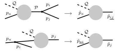
Figure 1: Kinematics for FE-IS (upper) and IE-FS (lower).

The remaining dipoles in (4) read

$$D_{i,j,a}^{\left(A\right)}\left(\tilde{p}_{\underline{ai}};\mathfrak{p}_{A}\right)=-\frac{1}{\left(p_{a}-p_{i}\right)^{2}-m_{\underline{ai}}^{2}}\,\frac{1}{x}\\ \big{<}\mathcal{M}_{n}\left(\tilde{p}_{\underline{ai}};\mathfrak{p}_{A}\right)\big{|}\frac{\hat{T}_{j}\!\cdot\!\hat{T}_{\underline{ai}}}{\hat{T}_{\underline{ai}}^{2}}\,\hat{V}_{a\rightarrow\underline{ai}\,i,\,j}^{\left(A\right)}\big{|}\mathcal{M}_{n}\left(\tilde{p}_{\underline{ai}};\mathfrak{p}_{A}\right)\big{>},$$ (5a)

$$D_{i,j,a}^{\left(B\right)}\left(\tilde{p}_{a};\mathfrak{p}_{B}\right)=-\frac{1}{\left(p_{i}+p_{j}\right)^{2}-m_{\underline{ij}}^{2}}\,\frac{1}{x}\\ \big{<}\mathcal{M}_{n}\left(\tilde{p}_{a};\mathfrak{p}_{B}\right)\big{|}\frac{\hat{T}_{a}\!\cdot\!\hat{T}_{\underline{ij}}}{\hat{T}_{\underline{ij}}^{2}}\,\hat{V}_{\underline{ij}\rightarrow i\,j,\,a}^{\left(B\right)}\big{|}\mathcal{M}_{n}\left(\tilde{p}_{a};\mathfrak{p}_{B}\right)\big{>},$$ (5b)

where $\big{|}\mathcal{M}_{n}\big{>}$ is a vector in helicity and color space such that $\left|\mathcal{M}_{n}\right|^{2}=\big{<}\mathcal{M}_{n}\big{|}\mathcal{M}_{n}\big{>}$ is a matrix element squared, summed/averaged over colors and spins (see (Catani and Seymour, 1997) for details). The kinematics is depicted in Fig. 1. For IE-FS the partons $a,\,i$ are replaced by a single parton $\underline{ai}$, while for FE-IS $i,\,j$ are replaced by $\underline{ij}$. Also the spectators acquire new momenta. All the new momenta in $\mathcal{M}_{n}$ are constructed to be on shell and satisfy the momentum conservation, also away from the IR limits. We adorn these new momenta with tilde. The resulting sets of final state momenta in $\mathcal{M}_{n}$ are denoted by $\mathfrak{p}_{A}$ and $\mathfrak{p}_{B}$, respectively.

The $x$ variable is the Sudakov longitudinal fraction of $\tilde{p}_{a}$ or $\tilde{p}_{\underline{ai}}$ along $p_{a}$ and the color operators $\hat{T}_{l}$ pick up relevant color factors and account for color correlations. The dipole splitting functions $\hat{V}$ act in the helicity space and account for spin correlations. In the quasi-collinear limit they tend to massive generalizations of splitting matrices, while in the soft limit they collapse to eikonal factors.

II.1 Dipole splitting functions

Here we present the realization of $\hat{V}$ in a general massive case. It is worth mentioning that our results extend those of Ref. (Catani et al., 2002), and coincide in suitable limits with the partially massless cases considered there.

First, let us define the tilded momenta as follows

$$\textrm{IE-FS:}\quad\tilde{p}_{j}^{\mu}=\tilde{w}_{A}\,\mathcal{P}^{\mu}-\tilde{u}_{A}\,p_{a}^{\mu},\quad\tilde{p}_{\underline{ai}}^{\mu}=\tilde{p}_{j}^{\mu}-\mathcal{Q}^{\mu},$$ (6a)

$$\textrm{FE-IS:}\quad\tilde{p}_{\underline{ij}}^{\mu}=\tilde{w}_{B}\,\mathcal{P}^{\mu}-\tilde{u}_{B}\,p_{a}^{\mu},\quad\tilde{p}_{a}^{\mu}=\tilde{p}_{\underline{ij}}^{\mu}-\mathcal{Q}^{\mu},$$ (6b)

where $\mathcal{P}=p_{i}+p_{j}$, $\mathcal{Q}=\mathcal{P}-p_{a}$ (Fig. 1) and $\tilde{u}$, $\tilde{w}$ variables are calculated from the on-shell conditions. In the soft limit $\tilde{u}\rightarrow 0$, $\tilde{w}\rightarrow 1$. Moreover $\tilde{u}\rightarrow 1-x$ in the quasi-collinear limit.

Let us now list our dipole splitting functions starting with IE-FS case. For a gluon emission $\mathbf{Q}\rightarrow\mathbf{Q}g$ (or $\overline{\mathbf{Q}}\rightarrow\overline{\mathbf{Q}}g$) we have (with $m_{\mathbf{Q}}\equiv m_{a}=m_{\underline{ai}}$, $m_{i}=0$)

$$\hat{V}_{\mathbf{Q}\rightarrow\mathbf{Q}g,\,j}^{\left(A\right)}=8\pi\mu_{\mathrm{r}}^{2\varepsilon}\alpha_{s}c_{\mathrm{F}}\\ \left[\frac{2}{\tilde{u}_{A}\tilde{v}_{j}^{2}+\tilde{z}}+\left(1-\varepsilon\right)\tilde{u}_{A}-2-\frac{1-\tilde{u}_{A}}{\tilde{z}}\,\frac{m_{\mathbf{Q}}^{2}}{\mathcal{P}_{a}}\right],$$ (7)

where $\tilde{z}=p_{i}\cdot p_{a}/\mathcal{P}_{a}$ with $\mathcal{P}_{a}=\mathcal{P}\cdot p_{a}$. Further, $\mu_{\mathrm{r}}$ is a mass scale needed in $D=4-2\varepsilon$ dimensions, and $\tilde{v}_{j}=\sqrt{1-\left(m_{a}m_{j}/\tilde{\gamma}\right)^{2}}$ with $\tilde{\gamma}=\tilde{p}_{j}\cdot p_{a}$. Above (and in what follows) the unit matrix in helicity space is suppressed.

For the $g\rightarrow\mathbf{Q}\overline{\mathbf{Q}}$ splitting we get

$$\hat{V}_{g\rightarrow\mathbf{Q}\overline{\mathbf{Q}},\,j}^{\left(A\right)}=8\pi\mu_{\mathrm{r}}^{2\varepsilon}\alpha_{s}T_{\mathrm{R}}\\ \left[1-\frac{1}{1-\varepsilon}\,\left(2\tilde{u}_{A}\left(1-\tilde{u}_{A}\right)-\frac{1-\tilde{u}_{A}}{\tilde{z}}\,\frac{m_{\mathbf{Q}}^{2}}{\mathcal{P}_{a}}\right)\right],$$ (8)

with the configuration of masses $m_{a}=0$, $m_{\mathbf{Q}}\equiv m_{\underline{ai}}=m_{i}$. Note that although the initial state parton is massless, this splitting is not present in (Dittmaier, 2000; Catani et al., 2002).

Finally for $\mathbf{Q}\rightarrow g\mathbf{Q}$, where a heavy quark is radiated, we have (with $m_{a}=m_{i}=m_{\mathbf{Q}}$, $m_{\underline{ai}}=0$)

$$\left(\hat{V}_{\mathbf{Q}\rightarrow g\mathbf{Q},\,j}^{\left(A\right)}\right)^{\mu\nu}=8\pi\mu_{\mathrm{r}}^{2\varepsilon}\alpha_{s}c_{\mathrm{F}}\left(1-\varepsilon\right)\\ \left[-g^{\mu\nu}\left(1-\tilde{u}_{A}\right)+\frac{4}{1-\tilde{u}_{A}}\,\frac{\mathcal{V}_{A}^{\mu}\mathcal{V}_{A}^{\nu}}{2\tilde{z}\mathcal{P}_{a}-m_{\mathbf{Q}}^{2}}\right].$$ (9)

The correlation tensor $\mathcal{V}_{A}^{\mu}\mathcal{V}_{A}^{\nu}$ is defined by

$$\mathcal{V}_{A}^{\mu}=\left(1-\tilde{z}\right)p_{i}^{\mu}-\tilde{z}p_{j}^{\mu}\\ +\left[m_{\mathbf{Q}}^{2}-m_{j}^{2}+\mathcal{P}^{2}\left(1-2\tilde{z}\right)\right]\frac{1-\tilde{w}_{A}}{2\tilde{p}_{\underline{ai}}\cdot\mathcal{P}}\,\mathcal{P}^{\mu}.$$ (10)

It fulfills transversality relation $\tilde{p}_{\underline{ai}}\cdot\mathcal{V}_{A}=0$.

Now let us turn to the FE-IS case. Here the difference with (Catani et al., 2002) is that the initial state spectator can be massive. For $\mathbf{Q}\rightarrow\mathbf{Q}g$ with $m_{i}=0$, $m_{j}=m_{\underline{ij}}=m_{\mathbf{Q}}$ we have

$$\hat{V}_{\mathbf{Q}\rightarrow\mathbf{Q}g,\,a}^{\left(B\right)}=8\pi\mu_{\mathrm{r}}^{2\varepsilon}\alpha_{s}c_{\mathrm{F}}\\ \left[\frac{2}{\tilde{u}_{B}\tilde{v}_{\mathbf{Q}}^{2}+\tilde{z}}+\left(1-\varepsilon\right)\tilde{z}-2-\frac{m_{\mathbf{Q}}^{2}}{p_{i}\cdot p_{j}}\right],$$ (11)

Further for $g\rightarrow\mathbf{Q}\overline{\mathbf{Q}}$ with $m_{\underline{ij}}=0$, $m_{i}=m_{j}=m_{\mathbf{Q}}$ we define

$$\left(\hat{V}_{g\rightarrow\mathbf{Q}\overline{\mathbf{Q}},\,a}^{\left(B\right)}\right)^{\mu\nu}=8\pi\mu_{\mathrm{r}}^{2\varepsilon}\alpha_{s}T_{\mathrm{R}}\left(-g^{\mu\nu}-4\frac{\mathcal{V}_{B}^{\mu}\mathcal{V}_{B}^{\nu}}{\mathcal{P}^{2}}\right),$$ (12)

with

$$\mathcal{V}_{B}^{\mu}=\tilde{z}p_{i}^{\mu}-\left(1-\tilde{z}\right)p_{j}^{\mu}-\frac{\tilde{u}_{B}m_{a}^{2}}{2\tilde{w}_{B}\mathcal{P}_{a}}\left(p_{i}^{\mu}-p_{j}^{\mu}\right)$$ (13)

satisfying $\tilde{p}_{\underline{ij}}\cdot\mathcal{V}_{B}=0$.

Finally for the $g\rightarrow gg$ splitting we have

$$\left(\hat{V}_{g\rightarrow gg,\,a}^{\left(B\right)}\right)^{\mu\nu}=16\pi\mu_{\mathrm{r}}^{2\varepsilon}\alpha_{s}c_{\mathrm{A}}\Bigg{[}-g^{\mu\nu}\Bigg{(}\frac{1}{1-\tilde{z}+\tilde{u}_{B}}\\ +\frac{1}{\tilde{z}+\tilde{u}_{B}}-2\Bigg{)}+2\left(1-\varepsilon\right)\frac{\mathcal{V}_{B}^{\mu}\mathcal{V}_{B}^{\nu}}{\mathcal{P}^{2}}\Bigg{]}.$$ (14)

Despite the massless splitting the above function gains some massive factors from spectator via the $\mathcal{V}_{B}^{\mu}$ vectors.

II.2 Dipole integration

The phase space factorization required in Eq. (2) is actually realized as a convolution in $\tilde{u}$ treated as a free variable. In this context we denote it by $u$ (without tilde). The construction requires dropping on-shell conditions for $\tilde{p}_{j}$ in IE-FS or $\tilde{p}_{\underline{ij}}$ in FE-IS cases and fixing two invariants $\mathcal{X}$, $\mathcal{Y}$, such that we can determine $\tilde{w}=\tilde{w}\left(u,\mathcal{X},\mathcal{Y}\right)$. Let us denote the corresponding off-shell vectors as $\tilde{p}_{j}\left(u,\mathcal{X},\mathcal{Y}\right)\equiv\tilde{p}_{j}\left(u\right)$, $\tilde{p}_{\underline{ij}}\left(u,\mathcal{X},\mathcal{Y}\right)\equiv\tilde{p}_{\underline{ij}}\left(u\right)$.

Our version of PS factorization formula has the form (for IE-FS case)

$$d\Phi_{n+1}\left(q,p_{a};\left\{p_{l}\right\}_{l=1}^{n+1}\right)=\\ \int\!\!du\,d\Phi_{n}\left(\mathcal{Q},\tilde{p}_{\underline{ai}}\left(u\right);\mathfrak{p}_{A}\right)\,d\phi_{a\rightarrow\underline{ai}\,i,\,j}^{\left(A\right)}\left(u\right),$$ (15)

where the arguments of the reduced phase space $d\Phi_{n}$ are the incoming and outgoing momenta (separated by semicolon). The subspace measure is

$$d\phi_{a\rightarrow\underline{ai}\,i,\,j}^{\left(A\right)}\left(u\right)=v^{3-D}\,\left(\mathcal{P}^{2}\right)^{\frac{D}{2}-2}\mathcal{J}\,\\ \left[\left(\tilde{z}_{+}-\tilde{z}\right)\left(\tilde{z}-\tilde{z}_{-}\right)\right]^{\frac{D}{2}-2}\,\frac{d\Omega_{D-2}d\tilde{z}}{4\left(2\pi\right)^{D-1}},$$ (16)

where $v=\sqrt{1-m_{a}^{2}\mathcal{P}^{2}/\mathcal{P}_{a}^{2}}$ and $d\Omega_{D-2}$ is a solid angle on transverse hyperplane in the $\mathcal{Q}$-$p_{a}$ CM system. The jacobian reads

$$\mathcal{J}=\left|\frac{\partial\tilde{p}_{j}^{2}\left(u\right)}{\partial u}\right|_{\mathcal{X},\mathcal{Y}},$$ (17)

with subscripts corresponding to variables kept fixed during differentiation. The bounds on $\tilde{z}$ are $\tilde{z}_{\pm}=\frac{1}{2}\left(1+\overline{m}_{i}^{2}-\overline{m}_{j}^{2}\pm 2v\overline{p}\right)$, where $\overline{p}=\frac{1}{2}\sqrt{1-2\left(\overline{m}_{i}^{2}+\overline{m}_{j}^{2}\right)+\left(\overline{m}_{i}^{2}-\overline{m}_{j}^{2}\right)^{2}}$ and the barred masses are rescaled by $\mathcal{P}^{2}$.

An analogous formula can be obtained for the FE-IS case. One has to replace the set $\mathfrak{p}_{A}$ by $\mathfrak{p}_{B}$ and make replacements: $\tilde{p}_{\underline{ai}}\leftrightarrow\tilde{p}_{a}$ in $d\Phi_{n}$ and $\tilde{p}_{j}\rightarrow\tilde{p}_{\underline{ij}}$ in the jacobian $\mathcal{J}$.

The choice of invariants $\mathcal{X}$, $\mathcal{Y}$ affects the PS generation in $d\Phi_{n}$ and ‘plus-distributions’ handling in the integrals over $d\phi$. In the following we take $\mathcal{X}=\tilde{\gamma}$, $\mathcal{Y}=\mathcal{P}_{a}$.

We note that in the desired integral $\int d\phi\,D$, with $D$ given in (5), only $\hat{V}$ and the propagators can depend on $\tilde{z}$. Further, it can be shown that, thanks to the gauge invariance and properties of $\mathcal{V}_{A,B}^{\mu}$, the helicity correlations in (5) vanish after integration. Therefore the integral over $d\Omega_{D-2}$ is trivial and we are left with a color correlated matrix element and a scalar function, which e.g. for IE-FS reads

$$I_{a\rightarrow\underline{ai}\,i,\,j}^{\left(A\right)}\left(u\right)=-\int\!\!d\phi_{a\rightarrow\underline{ai}\,i,\,j}^{\left(A\right)}\,\,\frac{\left\langle\hat{V}_{a\rightarrow\underline{ai}\,i,\,j}^{\left(A\right)}\right\rangle}{\left(p_{a}-p_{i}\right)^{2}-m_{\underline{ai}}^{2}}\,,$$ (18)

where $\left\langle\ldots\right\rangle$ denotes average over helicities in $D$ dimensions. The formula for FE-IS is analogous.

All the integrals have been calculated analytically in $D$ dimensions (Kotko, 2012; *Kotko:2012kw), and the details will be given in a forthcoming paper.

As an example, let us present the result for the IE-FS $g\rightarrow\mathbf{Q}\overline{\mathbf{Q}}$ dipole integral as we shall make use of it in Section III. In the $D=4$ limit we get

$${I}_{g\rightarrow\mathbf{Q}\overline{\mathbf{Q}},\,j}^{(A)}\left(u\right)=\frac{\eta_{\mathcal{J}}^{2}}{2\eta_{\mathcal{P}_{a}}^{4}}\,\\ \times\Bigg{\{}\eta_{\mathcal{P}_{a}}^{2}P_{gq}\left(u\right)\,\log\frac{\eta_{\mathbf{Q}}^{2}-\eta_{j}^{2}+\eta_{\mathcal{P}^{2}}^{2}\left(1+2\overline{p}\right)}{\eta_{\mathbf{Q}}^{2}-\eta_{j}^{2}+\eta_{\mathcal{P}^{2}}^{2}\left(1-2\overline{p}\right)}\\ +\frac{8\,T_{\mathrm{R}}\,\eta_{\mathbf{Q}}^{2}\,\eta_{\mathcal{P}^{2}}^{4}\left(1-u\right)\overline{p}}{\left(\eta_{\mathbf{Q}}^{2}-\eta_{j}^{2}+\eta_{\mathcal{P}^{2}}^{2}\right)^{2}-4\eta_{\mathcal{P}^{2}}^{4}\overline{p}^{2}}\Bigg{\}},$$ (19)

where $P_{gq}\left(u\right)=T_{\mathrm{R}}\left[1-2u\left(1-u\right)\right]$ is the standard splitting function, $\eta_{j}^{2}=m_{j}^{2}/2\tilde{\gamma}$, $\eta_{\mathbf{Q}}^{2}=m_{\mathbf{Q}}^{2}/2\tilde{\gamma}$ and other $\eta^{2}_{X}=X/2\tilde{\gamma}$ for $X=\mathcal{P}_{a},\mathcal{P}^{2},\mathcal{J}$. Note that in the above formula a non-trivial dependence on $u$ is hidden in $\overline{p}$ and $\eta^{2}_{X}$.

III Factorization of (quasi-)singularities

In general, the integrated dipole functions contain IR poles, which get canceled upon including virtual corrections. There are no further singularities in the massive case. Nevertheless, some IR sensitive terms (q-singularities) still remain in the IE-FS dipoles, and we factorize them out by subtracting counterterms (3) according to the ACOT scheme, as we explain below.

Let us consider the integrated IE-FS dipole in the limit of vanishing mass of the emitter or emitted parton (the spectator $j$ can remain massive). For instance, using Eq. (19), we obtain

$$I_{g\rightarrow\mathbf{Q}\overline{\mathbf{Q}},\,j}^{\left(A\right)}\left(u\right)=\frac{\alpha_{s}}{2\pi}\Bigg{[}P_{gq}\left(u\right)\Bigg{(}\log\frac{u^{2}}{u+\eta_{j}^{2}}-\log\eta_{\mathbf{Q}}^{2}\Bigg{)}\\ +2T_{\mathrm{R}}\,u\left(1-u\right)\Bigg{]}+\mathcal{O}\left(\eta_{\mathbf{Q}}^{2}\right),$$ (20)

The counterterms $\mathcal{C}_{n,a}$ are given in terms of the partonic densities $\mathcal{F}_{ab}$, which are defined via matrix elements of bilocal operators on the light-cone and can be calculated perturbatively. The emerging UV singularities have to be renormalized which, in turn, specifies the evolution kernels for PDFs (see (Collins, 2011) for a review).

According to the ACOT scheme, this standard procedure can also be used with massive quarks (Collins, 1998). In particular, one can still define partonic PDFs and renormalize them using $\overline{\mathrm{MS}}$, assuring standard DGLAP evolution equations (actually one uses the composite CWZ renormalization scheme (Collins et al., 1978)). For asymptotically large $Q^{2}$, the above construction leads to the standard $\overline{\mathrm{MS}}$ calculation. On the other hand, when $Q^{2}\simeq m^{2}_{\mathbf{Q}}$ the $\mathit{C}_{n,a}$ counterterms approximately cancel the $\sigma^{(\mathrm{LO})}$ contribution, basically resulting in the ‘fixed order’ description (Aivazis et al., 1994).

Using the Feynman rules for PDFs (Collins and Soper, 1982; Collins, 2011) one can show that in the $\overline{\mathrm{MS}}$ scheme

$$\mathcal{F}_{g\mathbf{Q}}\left(z\right)=\frac{\alpha_{s}}{2\pi}\,T_{\mathrm{R}}\,\left(1-2z\left(1-z\right)\right)\,\log\frac{\mu_{\mathrm{r}}^{2}}{m_{\mathbf{Q}}^{2}}\,,$$ (21)

$$\mathcal{\mathcal{F}}_{\mathbf{Q}g}\left(z\right)=\frac{\alpha_{s}}{2\pi}\,c_{\mathrm{F}}\,\frac{1+\left(1-z\right)^{2}}{z}\\ \left[\log\frac{\mu_{\mathrm{r}}^{2}}{m_{\mathbf{Q}}^{2}}-2\log z-1\right]$$ (22)

$$\mathcal{\mathcal{F}}_{\mathbf{Q}\mathbf{Q}}\left(z\right)=\frac{\alpha_{s}}{2\pi}\,c_{\mathrm{F}}\\ \left\{\frac{1+z^{2}}{1-z}\left[\log\frac{\mu_{\mathrm{r}}^{2}}{m_{\mathbf{Q}}^{2}}-2\log\left(1-z\right)-1\right]\right\}_{+},$$ (23)

$$\mathcal{F}_{gg}\left(z\right)=\frac{\alpha_{s}}{2\pi}\,\\ \Bigg{\{}2c_{\mathrm{A}}\,\left[\left(\frac{1}{1-z}\right)_{+}+\frac{1-z}{z}-1+z\left(1-z\right)\right]\\ +\delta\left(1-z\right)\left(\frac{11}{6}c_{\mathrm{A}}-\frac{2}{3}N_{\mathrm{f}}\,T_{\mathrm{R}}-\frac{2}{3}T_{\mathrm{R}}\log\frac{\mu_{\mathrm{r}}^{2}}{m_{\mathbf{Q}}^{2}}\right)\Bigg{\}}.$$ (24)

where $z$ is the fractional momentum of parton $b$.

We have checked that using $\mathcal{C}_{n,a}$ with the above $\mathcal{F}_{ab}$ (intermediate steps require usage of color conservation for $\hat{T}_{j}$ operators) we get IR safe dipoles. Moreover, in the considered limit we get the same dipoles as those of Ref. (Catani et al., 2002) with the standard massless collinear subtraction term (i.e. with $\mathcal{F}_{ab}\left(z\right)=-\alpha_{s}P_{ab}\left(z\right)/2\pi\varepsilon$).

There is one comment in order. Certain ambiguities (Collins, 1998) of the ACOT scheme stimulated construction of the so called Simplified ACOT (S-ACOT) scheme (Kramer et al., 2000), where all initial state masses are set to zero. This scheme is convenient for higher order calculations (Stavreva et al., 2012), which otherwise are very cumbersome. Our approach is however different as it operates on more exclusive quantities, hence we resolve the ambiguities differently. Namely, we set the initial state masses to zero in $\sigma^{(\mathrm{LO})}$ and in the $\mathcal{C}_{n,a}$ contribution to $\sigma^{(\mathrm{NLO})}$. This results in massless integration limits in the corresponding convolutions, in analogy to the standard DGLAP evolution equations. This approach is not strictly required by our formalism, but provides a better transition to the ‘fixed order’ description, cf. solid and dotted lines in Fig. 2. We point out that we do not set any other masses to zero, neither for initial nor for the final states. If, however, one wants to use the S-ACOT scheme for jets, then only the dipoles for the $g\rightarrow\mathbf{Q}\overline{\mathbf{Q}}$ initial state splitting are needed.

IV Numerical tests

We have partially implemented our method in a dedicated C++ program. The MC integration and event generation is accomplished using the FOAM engine (Jadach, 2003).

In order to test our approach, we have used our program to numerically calculate a quantity which can be obtained independently, namely the charm structure function $F_{2c}$.

The LO contribution comes from $\gamma\mathbf{Q}\rightarrow\mathbf{Q}$ (plus the same with $\overline{\mathbf{Q}}$). The real NLO corrections are $\gamma\mathbf{Q}\rightarrow\mathbf{Q}g$ and $\gamma g\rightarrow\mathbf{Q}\overline{\mathbf{Q}}$, while the virtual ones are given e.g. in (Kretzer and Schienbein, 1998).

In order to perform the numerical integration we need three distinct dipoles $D_{\mathbf{Q},\overline{\mathbf{Q}},g}^{\left(A\right)}=D_{\overline{\mathbf{Q}},\mathbf{Q},g}^{\left(A\right)}$, $D_{g,\mathbf{Q},\mathbf{Q}}^{\left(A\right)}=D_{g,\overline{\mathbf{Q}},\overline{\mathbf{Q}}}^{\left(A\right)}$, $D_{g,\mathbf{Q},\mathbf{Q}}^{\left(B\right)}=D_{g,\overline{\mathbf{Q}},\overline{\mathbf{Q}}}^{\left(B\right)}$ as well as their integrals. Since there are two IE-FS dipoles we need two collinear subtraction terms with corresponding $\mathcal{F}_{g\mathbf{Q}}$ and $\mathcal{F}_{\mathbf{Q\mathbf{Q}}}$.

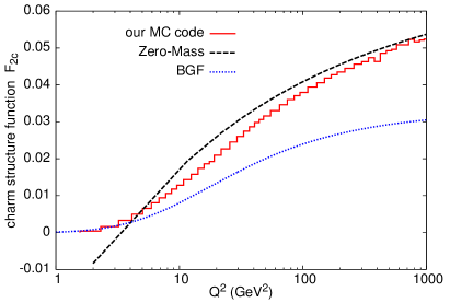
Figure 2: The charm structure function, $F_{2c}$, calculated in different schemes: GM from our MC code at NLO (red solid line), Zero-Mass at NLO (black dashed line), Fixed Order (BGF) at ${\cal O}(\alpha_{\mathrm{s}})$ (blue dotted line). The calculations were done using CTEQ5 PDFs at $x_{\rm B}=0.05$.

We observe, that the soft poles coming from virtual corrections cancel against the sum of soft poles coming from IE-FS and FE-IS dipoles. The result of numerical integration perfectly agrees with the semi-analytical formula calculated independently according to (Aivazis et al., 1994; Kretzer and Schienbein, 1998). In Fig. 2 we show that our result indeed interpolates between the massless NLO calculation at high $Q^{2}$ and the fixed order, ${\cal O}(\alpha_{\mathrm{s}})$, calculation at low $Q^{2}$. Let us stress that this result is obtained by the MC integration of a fully differential cross section (2).

This is clearly the first simplest test. It verifies only a part of the dipoles and collinear counterterms. More tests are due in course of the code development.

V Summary

In the present paper we have briefly described — without going into technical details — a general mass scheme for jet production in DIS. The scheme is based on the ACOT factorization theorem which is proved to all orders. The proof is constructed for structure functions, but it actually holds for all IR safe quantities. This entitles us to use this factorization scheme for jets, provided we have a suitable dipole subtraction method that can deal with heavy quarks in the initial state. We have constructed such a method, generalizing the existing results. We have checked that this method removes all potential collinear singularities as desired, and that the remaining dipoles coincide with those of the massless calculation in $\overline{\mathrm{MS}}$.

All the crucial calculations are already performed (Kotko, 2012; *Kotko:2012kw) and the details shall be presented in a separate publication. The computer code suitable for the jet production in DIS is under construction.

An extension to hadron-hadron collisions is, in principle, straightforward. Formally, one only needs to introduce an additional class of dipoles for the initial state emitter and initial state spectator. Nonetheless, we are aware of challenges arising at higher orders (above NLO) — like the feasibility of dipole subtraction method or non-cancellation of soft singularities when two initial state partons are massive. These issues have been widely discussed in literature, but practical procedures still have to be analyzed.