Rectangular Wilson Loops at Large N

Abstract:

This work is about pure Yang-Mills theory in four Euclidean dimensions with gauge group $\operatorname{SU}(N)$. We study rectangular smeared Wilson loops on the lattice at large $N$ and relatively close to the large-$N$ transition point in their eigenvalue density. We show that the string tension can be extracted from these loops but their dependence on shape differs from the asymptotic prediction of effective string theory.

1 Introduction

This article is about Wilson loop operators, $W(\operatorname{\cal C})$, in four-dimensional Euclidean $\operatorname{SU}(N)$ pure gauge theory. $\operatorname{\cal C}$ is a closed, non-self-intersecting continuous curve in $\mathbb{R}^{4}$, differentiable except at a finite set of points where there are finite discontinuities in the unit tangent vector to the curve. $W(\operatorname{\cal C})$ is well defined only after a renormalization that eliminates perimeter and corner divergences.

The inclusion of kinks is a complication one would like to avoid in initial studies. It becomes essential if one wants to make the Makeenko-Migdal equations well defined. It also is needed if one wishes to employ lattice field theory tools to validate non-perturbative assumptions about $W(\operatorname{\cal C})$ for contractible $\operatorname{\cal C}$.

1.1 Smearing

A convenient way to renormalize $W(\operatorname{\cal C})$ is to use continuum smearing, henceforth referred to as “smearing”. Smearing is a well defined procedure in Euclidean continuum field theory, abstracting some more ad-hoc procedures in common use in lattice field theory. It was introduced in [1] and a brief review of its history can be found in [2]. Smearing introduces an extra parameter, $s$, of dimension length squared. $\sqrt{s}$ is an observer’s resolution of localized objects constructed out of fields. Keeping this resolution nonzero eliminates all divergences associated with operator compositeness. Smearing enjoys several useful properties:

• All standard general regularization methods (purely perturbative or lattice) are compatible with smearing. Perturbatively, the counter terms to the classical Lagrangian required by ordinary renormalization make all observables constructed out of only smeared fields finite – with no restriction on their space-time arguments. Beyond perturbation theory, choosing some reasonable definition of a scale eliminates ultraviolet divergences from all smeared observables.

• $\rm O(4)$ spacetime invariance remains preserved if the regularization preserves it.

• Gauge invariance remains preserved if the regularization preserves it.

• For any $\operatorname{\cal C}$, smearing provides a proper definition of the joint eigenvalue distribution of parallel transport round $\operatorname{\cal C}$ and these eigenvalues reside on the unit circle. The concept of a marginal probability distribution for the parallel transport unitary matrix round $\operatorname{\cal C}$ in the continuum limit makes sense only after smearing. The classical view of parallel transport as an element in the compact $\operatorname{SU}(N)$ group is preserved at the quantum renormalized level thanks to smearing, but won’t hold with more standard methods of continuum regularization. In particular if we allow $\operatorname{\cal C}$ to have an exactly backtracking segment, subsequent passages will cancel exactly out at the quantum level. Smeared Wilson loops obey Polyakov’s [3] zigzag symmetry.

• At the formal level of the Makeenko-Migdal loop equations, the definition of smearing can be extended to loop space [4]. In this formal sense, smearing is defined without any reference to the gauge fields and their Lagrangian. The smearing parameter plays the role of the evolution variable in a generalization of diffusion to loop space.

• Small smeared Wilson loops admit a local expansion [2] with well defined “condensates” at each order. These condensates can be rendered dimensionless by multiplication by a power of $s$. These dimensionless numbers provide non-perturbative definitions of “running” coupling constants at scale $s$. Unlike their phenomenological progenitors [5], [6], the condensates are well defined. They have a calculable perturbative expansion. The terms in this expansion do not vanish. Another way to define “condensates” is from the large-momentum structure of a specific observable [7]. Such a definition does not ensure that precisely the same condensate enters in other observables. The smeared versions are defined in a manner independent of the observable. They are dependent on the smearing parameter. This parameter is denoted by $s$ in the continuum and by $S$ on the lattice.

Admittedly, smearing is an artificial device. We do not know of an alternative construction of a full set of functionals $W(\operatorname{\cal C})$ with properties listed above.

Preserving the full $\rm O(4)$ symmetry of space-time in the process of smearing has the drawback that smeared correlation functions will not exhibit the unitarity of the underlying theory in a transparent manner. For those quantities that have a finite limit as $s\to 0$ transparency will be recovered. One can define a version of smearing which only preserves an $\rm O(3)$ subgroup of $\rm O(4)$ and thus keep unitarity evident. The cost is the loss of explicit Euclidean $\rm O(4)$ invariance.

It is important to keep in mind the distinction between the (continuous) smearing we are using here and more standard procedures. For example, in [8] smeared rectangular Wilson loops were used to extract the interquark potential and ultimately force. The smearing was restricted to three directions perpendicular to the “time” direction, which was taken to infinity. The smearing was done by iteratively adding one-plaquette-windowed paths to the spatial portions of the loop with a weight of 1/2.

Thus, this older version of smearing differs on two counts from the continuous smearing we are employing in this paper: It is only $\rm O(3)$ invariant and it is defined only on the lattice.

The proper way to think about this smearing is as a procedure to improve the numerical quality of the string energies defined in the asymptotic large-time regime. This smearing is a purely lattice technique and plays no role in the subsequent extraction of physically relevant parameters. No remnant of this smearing is left in the continuum limit.

The smearing we use in this work is intentionally designed to make the Wilson loop average itself well defined in the continuum, rather than just the interquark force. To achieve this an extra, tunable, dimensional parameter is introduced, intuitively describing the resolution at which the Wilson loop is observed.

1.2 Weakly versus strongly coupled regimes

In 4D $\operatorname{SU}(N)$ pure gauge theory, classical scale invariance is anomalous and gets broken at the quantum level. A scale separating a weakly coupled short distance regime from a qualitatively different strongly coupled long distance regime is dynamically generated. Observables admit an asymptotic expansion computable in perturbation theory at short distances. There are no systematic methods of analytic computation at large distances. These two regimes coexist in the same theory and are smoothly connected. The crossover is relatively narrow.

Numerical simulations have established that at large distance the theory confines. This is in agreement with experimental data for $N=3$. A strong version of the confinement postulate is: If we scale a loop $\operatorname{\cal C}$ up, $\operatorname{\cal C}\to\rho\operatorname{\cal C}$, $W(\rho\operatorname{\cal C})\sim\exp(-\rho^{2}\sigma A_{\rm min})$ as $\rho\to\infty$ with $A_{\rm min}$ the minimal area of all continuous surfaces in $\mathbb{R}^{4}$ bounded by $\operatorname{\cal C}$. The string tension $\sigma$ has dimension of mass squared and is universal: It does not depend on the shape of $\operatorname{\cal C}$. The numerical and the empirical evidence are both restricted to simpler loops. Typically, they fit in a plane inside Euclidean $\mathbb{R}^{4}$, are non-self-intersecting and not too unusually shaped.

The string tension can be extracted from unsmeared Wilson loops $W(\operatorname{\cal C},s=0)$ by numerical means. The externally determined resolution scale $\sqrt{s}$ can be thought of as representing an effective thickness of $\operatorname{\cal C}$. For very large loops the fixed finite thickness $\sqrt{s}$ should not enter. One expects $W(\rho\operatorname{\cal C},s)\sim\exp(-\sigma\rho^{2}A_{\rm min}(\operatorname{\cal C}))$ with $\sigma$ independent of $s$.

There does not exist so far a mathematically rigorous proof of confinement in the continuum limit. Even if we postulate confinement, there is no credible analytical computation of $\sigma$ in terms of a perturbatively defined scale $\Lambda$. We think methods of effective field/string theory could achieve this. In this paper we use the lattice to study in detail the crossover from weak to strong coupling. We hope to learn how to quantitatively connect the confinement regime to the weakly coupled one and eventually estimate $\sigma/\Lambda^{2}$ without using the lattice in any quantitative way.

The spirit is the same as in a semiclassical approximation based on instantons [9]. That approach was not successful but framed the problem well. It tried to connect the perturbative regime to a regime in which an MIT bag description held by a crossover described using an instanton gas. A more phenomenological approach was based on an extension of perturbative OPE to include nonperturbative contributions parametrized by “condensates” [5]. This approach was quite successful but is imprecisely defined. It remains unclear how a theorist would extract an exact value of a universally meaningful “condensate” even if she/he somehow managed to solve QCD exactly in the presence of an acceptable UV cutoff.

Perhaps it is not by accident that our concrete approach employs an artificial smearing scale. Smearing provides well defined candidates for SVZ condensates, as already mentioned. These condensates also are not directly physical since smearing is somewhat ad-hoc. They are universally meaningful though. They would be quantitatively useful only if one chose a reasonable level of smearing. A good choice would provide an economical parametrization of the short distance – long distance crossover.

This paper is part of a general strategy. We want to gain analytical control of the crossover for simple Wilson loops by exploiting newly established large-$N$ phenomena by computer simulation. Then we want to compute $\sigma$ in units of a perturbative scale $\Lambda^{2}$. Confinement is assumed and one accepts an effective description of the confinement regime based on the scale $\sigma$. This might become practical long before a mathematical proof of confinement is found and without a detailed understanding of what causes it.

1.3 Large $N$

The essence of the weak – strong coupling problem remains present in the limit $N\to\infty$. The limit is taken as $Ng_{N}^{2}(s)\equiv\lambda(s)$ is kept fixed [10]. $g_{N}^{2}(s)$ is a running coupling constant in some standard definition.

It has been recently established that the weak-strong crossover range collapses into a well defined point at infinite $N$ [4]. The transition point depends on the shape of $\operatorname{\cal C}$. As the loop $\operatorname{\cal C}$ is dilated at fixed non-zero smearing and shape a non-analytic change in the single-eigenvalue distribution takes place at a sharply defined scale. For a small loop the distribution is insensitive to the compact nature of $\operatorname{SU}(N)$. For a larger loop the full group is explored by the parallel transporter round it. For finite $N$ there is no non-analyticity and the full group is felt by parallel transport around all loops.

Group compactness is a key ingredient for confinement. Perturbation theory is insensitive to it because it starts from an infinite-range Gaussian integral over YM fields. The transition at which the eigenvalues of the parallel transport matrix “discover” the point in the group that is farthest from identity is a natural scale for matching perturbation theory to a long distance description. Traces of smeared Wilson loops in the fundamental representation remain smooth through the transition even at infinite $N$, although the single eigenvalue distribution is not analytic there. Therefore, traces of smeared Wilson loops should match well. The small loop regime is in principle calculable by field theory. More recently we have learned that one can also make predictions by analytical means about the large loop regime. The framework for doing that is effective string theory.

1.4 Effective string theory

Effective string theory [11], [12] bears conceptual similarity to the well known chiral effective field theory describing the interactions between soft pions in an $\operatorname{SU}(N)$ gauge theory with a moderate number of massless quarks. One assumes that spontaneous chiral symmetry breaking occurs via a bilinear condensate and that the finite non-zero pion decay constant $f_{\pi}$ is the scale typical for effects caused by this breaking. Then, symmetry considerations produce a large set of predictions. One has a proof [13] for chiral symmetry breaking at a physicist’s level of rigor but the proof provides no indication for how to calculate $f_{\pi}$ in terms of $\Lambda$ by analytical means. Consider the correlation function of two flavor currents in QCD. We have a perturbative description at short distances and a chiral effective field theory description at long distances [5], [14]. Joining them at a crossover scale would provide some estimates for the ratio $f_{\pi}^{2}/\Lambda^{2}$. Resonance contributions come in in the crossover regime and the match is complicated. The large-$N$ limit simplifies matters somewhat because the resonances become isolated stable particles coming in as poles.

The Wilson loop analogy is substantially less developed and we think that time has come to look into the problem of matching short to long distances for Wilson loops in some detail. The existence of the sharply demarcated matching point on the one hand and the smoothness of the observable through this matching point on the other are encouraging.

We want to determine by lattice gauge theory methods how an effective string description on the strong coupling side of the matching point and close to it works in detail. The effective string theory makes predictions for a functional of curves $\operatorname{\cal C}$ and the central assumption is that these predictions describe Wilson loops. The string tension $\sigma$ is used to set the scale in the theory from the outside. The effective string theory in itself does not generate any scale. An important issue is how this matching depends on scale-invariant features of $\operatorname{\cal C}$.

The predictions are obtained starting from a limit where the minimal spanning area of $\operatorname{\cal C}$ is very large. One can ignore any length scale that stays fixed as $\operatorname{\cal C}$ is dilated. Very large loops are described by the Nambu-Goto action for 2 massless bosonic fields. It is impossible to define this limiting theory exactly. This is not needed as an asymptotic expansion in inverse loop-size produces well defined terms without a full definition of the theory. The predictions made by effective string theory are obtained from the expansion of the action around its quadratic approximation. Eventually one reaches an order at which non-Nambu-Goto terms are needed. Unlike in the chiral Lagrangian case, this order appears to be relatively high. The main ingredient organizing the expansion is the postulated local nature of the world-sheet theory. Effective string theory for contractible Wilson loops and effective field theory for massless pions differ in scope. The effective chiral Lagrangian applies to functions of a finite number of scales, while effective string theory applies to a functional of a continuum of scales.

String theory would require the inclusion of handles in the calculation of corrections. It is believed that handles can be neglected at infinite $N$. Thus, in the ’t Hooft limit, one ends up using just purely field-theoretical methods of two-dimensional field theory when one imposes on the effective string description symmetry restrictions coming from the original theory.

In this numerical work we do not have data of quality needed to identify terms predicted by the effective string approach beyond the determinant of Gaussian surface fluctuations. The leading term states that as the loop is dilated to infinite size, at fixed shape, $\log W(\operatorname{\cal C},s)\sim-\sigma A_{\rm min}(\operatorname{\cal C})$. The two next subleading terms in the asymptotic expansion around very large loops come from the determinant of small fluctuations of the surface bounded by $\operatorname{\cal C}$ about its absolutely minimal area configuration. This configuration is assumed unique and well separated from other minima. The first subleading term is proportional to $\log(A_{\rm min})$ and the second is invariant under scalings of $\operatorname{\cal C}$. Except for simple contours, it won’t be possible to write down explicit formulas for the second subleading term, but, for any specific $\operatorname{\cal C}$, the value of the term can be obtained numerically with relative ease.

The effective string theory cannot make predictions for two terms that are present in $\log W(\operatorname{\cal C},s)$ and come in between its leading and its subleading predictions. These unpredictable terms consist of a perimeter term and a corner term. Both are smearing dependent. A potential problem then arises of an “interference” between further smearing-dependent subleading terms in $W(\operatorname{\cal C},s)$ and smearing independent terms coming from the effective string theory. The consequence of this “interference” is that even given an exact formula for $W(\operatorname{\cal C},s)$, coming from $\operatorname{SU}(N)$ field theory, we would not be able to check whether the effective string theory works or not because we would not be able to separate out the effective-string prediction. The higher-order effective-string predictions could then just “melt away” into the exact expression.

The field theory produces a $\log(W(\operatorname{\cal C},s))$ which diverges as $s\to 0$. The divergences appear in an asymptotic expansion at fixed $\operatorname{\cal C}$ in $s$ as $s\to 0$. Subtracting the $\operatorname{\cal C}$-dependent terms that go as $\frac{1}{\sqrt{s}}$ and $\log^{\kappa}{s\Lambda^{2}}$ would yield a finite expression. $\kappa=1$ at tree level in perturbation theory and subsequent terms in the leading log approximation can be resummed using the Callan-Symazik equation. This produces a term going like $\log(\log s\Lambda^{2})$.

Let us consider the case of a very small smearing parameter first: $s\sigma\ll 1$. It makes sense now to just subtract terms that diverge as $s\to 0$ and then set $s=0$. This would produce as “pure” a Wilson loop as any other regularization, which does not involve smearing, would. The power divergence is a perimeter term, well separated from other terms. It is clear how to subtract it without introducing finite terms that depend on the curve. There are no logarithmic divergences proportional to the perimeter. The subtraction of the logarithmic divergence depends on the opening angles of the corners. It is unclear how to disentangle the remaining finite parts from the subtraction of the corner divergences from unrelated terms dependent on shape features of $\operatorname{\cal C}$. By definition we are considering an asymptotic expansion in a parameter describing by how much the Wilson loop has been dilated relative to a standard size. The coefficients in the asymptotic expansion in the inverse of the dilation parameter are nontrivial functions of the shape of the loop, which is kept constant throughout. Effective string theory can be used to provide expressions for these coefficients. These expressions consist of functions of loop shape, but not overall scale. This particular asymptotic expansion differs from other variants, which also are produced by effective string theory. For example, one might extract the interquark force from rectangular loops and consider the expansion of this force in the distance between the quarks measured in units of the string tension, $\sqrt{\sigma}R$. Now the coefficients are just pure numbers.

In our context we are left with an open question as to what effective string theory predictions for the dependence on shape parameters of $\operatorname{\cal C}$ should be compared to. One of our objectives in this paper is to get some guidance on this question from numerical simulation.

2 Rough outline of paper

We have obtained Monte Carlo estimates for smeared rectangular Wilson loops on a hypercubic lattice at various smearing levels, $N$’s, couplings, volumes and combinations of rectangle sides. The estimates were obtained using a data base of 160 uncorrelated equilibrated gauge fields we have distributed on a forty node PC cluster. Each cluster node has four cores and a total of 24GB of memory to be able to smear and make measurements on four distinct gauge fields simultaneously.

Wilson loops in all distinct orientations and locations were averaged over for each gauge configuration separately. For each set of parameters defining the gauge field action and the loop we obtain 160 numbers. The set of these numbers is used for the statistical estimation of various physical parameters. Statistical errors are always determined by jackknife with the elimination of one single gauge configuration from the set of 160 at a time.

We start by extracting the string tension from square loops. The infinite-volume and large-$N$ limits on the lattice are dealt with first. Then the string tension is extrapolated to its continuum limit. The results and extrapolations are validated against a set of $L\times L\!+\!1$ and $L\times 2L$ loops. This analysis is done assuming that the term logarithmic in the area is precisely the one predicted by effective string theory but making no assumptions about the shape-dependent terms. This is achieved by ensuring that shape-dependent terms play no role at this stage. Under the same assumption about the logarithmic area dependence a loop-shape dependent number is extracted from the data and compared to the string prediction. The data is revisited and using global fits the coefficient of the logarithm of the area is determined. We obtain numbers consistent with the effective string theory value. This validates the assumption we made earlier when the coefficient was held fixed. The dependence on smearing is addressed throughout.

3 Parameter choices

We use the standard Wilson single-plaquette action. The standard coupling $\beta$ is incorporated into $b=\frac{\beta}{2N^{2}}$. The $N\to\infty$ limit is taken at fixed $b$. All our gauge configurations are on symmetric hypercubes of side $V^{\frac{1}{4}}$. $V$ is the total number of sites and the boundary conditions are periodic. We wish to use effective string theory to understand the data and the structure of the latter is restricted in the continuum by target space $\rm O(4)$ invariance. In order to maintain as much of the latter as possible at the regularized level we work only with symmetric volumes.

For large $N$ there is a bulk transition close to $b=0.360$. For substantially smaller values of $b$ the system is in a phase disconnected from continuum Yang-Mills theory. We also need to maintain $b\leq 0.369$ to be sure that spontaneous $Z^{4}(N)$ breaking at $N=\infty$ [15] is avoided on all our volumes, including our smallest, $12^{4}$. We mainly use the range of couplings $0.359\leq b\leq 0.369$. These couplings can produce relatively small and fine lattices. A judicious exploitation of continuum large-$N$ reduction allows us to always carry out the required extrapolation to infinite volume. Continuum large-$N$ reduction is sometimes also referred to as partial reduction. It is a conservative version of reduction introduced in [16]. Henceforth we shall use the term “reduction” instead of “continuum reduction”.

We stored statistically independent gauge fields at intervals $\Delta b=0.001$. Satisfactory statistical independence for our observables is obtained for gauge fields at neighboring $b$’s being separated by 500 complete $\operatorname{SU}(2)$ updates combined with 500 complete over-relaxation passes. The autocorrelation time is equal to about one quarter of this separation. The set of $N$ values we use consists of $N=7$, $11$, $13$, $19$, $29$. The computer time for generating a gauge field configuration goes as $N^{3}V$ and this is the primary limitation on the $(N,V)$ combinations we use.

Each measurement proceeds after the gauge fields have been smeared. The smearing parameter $S$ has mainly been taken in the range $0.2\leq S\leq 0.4$. In some cases we have data up to $S=0.52$. The separation between sequential smearing levels is $\Delta S=0.04$.

The Wilson loops $W_{N}$ on the lattice are defined by

$$W_{N}(L_{1},L_{2},b,S,V)=\frac{1}{N}\langle\operatorname{Tr}\prod_{{\it l}\in\operatorname{\cal C}}U_{{\it l}}\rangle\,.$$ (3.1)

The product is over the links ${\it l}$ in the order they appear when one goes once round $\operatorname{\cal C}$, a rectangle of sides $L_{1,2}$. All our fits will be applied to

$$w_{N}(L_{1},L_{2},b,S,V)=-\log W_{N}(L_{1},L_{2},b,S,V)\,.$$ (3.2)

When the loops are square the two variables $L_{1},L_{2}$ are replaced by one $L$ with the understanding that $L_{1,2}=L$.

4 Square loops

4.1 $N\to\infty$ and $V\to\infty$ limits

We first want to determine the limit

$$\lim_{N\to\infty}\left(\lim_{V\to\infty}w_{N}(L,b,S,V)\right)\,.$$ (4.1)

Numerically this is nontrivial since we need a good level of accuracy on the limit. Fits extracting physical parameters are applied to estimates for this limit.

Once $V$ is larger than some moderate $V_{c}(b)$, large-$N$ reduction provides in principle a shortcut allowing one to drop the limit $V\to\infty$ above. At which $N$ rough convergence is attained will depend on $V$. This requires numerical tests and fits. In addition to $N$, $V$, and $b$ the magnitude of finite-volume corrections also depends on the observable: the larger it is the bigger the finite-volume effects that need to be overcome are.

We use two different methods to compute the limit (4.1):

• Method 1)
  At fixed $N$ we compute $w_{N}$ on volumes that are sufficiently large for finite-volume effects to be negligible, then we determine $w_{\infty}(V=\infty)$ by fitting $w_{N}(V=\infty)$ to

  $$w_{N}(V=\infty)=w_{\infty}(V=\infty)+\frac{a_{1}(V=\infty)}{N^{2}}+\frac{a_{2}(V=\infty)}{N^{4}}\,.$$ (4.2)

  Here, the other arguments of $w$ are omitted for simplicity. All coefficients depend on the observable.
  We have evidence (strong for $N=7$ and $N=11$, not that strong for $N=19$ and rather weak for $N=29$) that volumes $V=24^{4}$, $18^{4}$, $14^{4}$, $12^{4}$ are sufficiently large for $N=7$, $11$, $19$, $29$, respectively. This statement applies to the specific set of couplings and loop sizes we use. The evidence comes from comparing to results on other volumes $V$ and/or other values of $N$ or even from trying to extrapolate from lower values of $b$. The accuracy of our data does not allow to quantify the finite-volume effects and we have to settle for something more qualitative. We managed to convince ourselves that the finite-volume systematical deviations are smaller than our statistical errors.

• Method 2)
  The second method makes use of large-$N$ reduction. At fixed $V$, we first take the limit $N\to\infty$ of $w_{N}(V)$ by fitting

  $$w_{N}(V)=w_{\infty}(V)+\frac{a_{1}(V)}{N^{2}}+\frac{a_{2}(V)}{N^{4}}\,.$$ (4.3)

  So long as the center symmetry stays unbroken, there is no volume dependence in the infinite-$N$ theory, i.e., $w_{\infty}(V)=w_{\infty}(V=\infty)$.
  We determine $w_{\infty}(V=12^{4})$ from $N=11$, $13$, $19$, $29$ [method 2a)] and $w_{\infty}(V=14^{4})$ from $N=7$, $11$, $13$, $19$ [method 2b)].

  There is little theoretical doubt that reduction indeed holds as a statement about $N=\infty$ for values of $(b,V)$ in the allowed region. The limit $N\to\infty$ is unlikely to be uniform in $(b,V)$ or in the size of the loop $\operatorname{\cal C}$ and in the level of smearing $S$. If we see good fits to a sum of terms decreasing as $\frac{1}{N^{2}}$ we know that we have taken into account subleading effects that do have a dependence on $V$. Only then can we trust that the leading term is indeed $V$-independent.

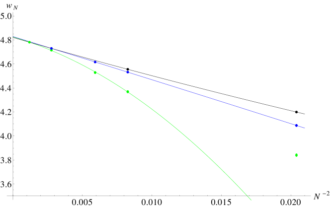
Figure 1: Plots of $w_{N}(L=9,b=0.368,S=0.4,V)$ as a function of $1/N^{2}$: $V=12^{4}$ in green, $V=14^{4}$ in blue and $V=24^{4}$ (at $N=7$), $V=18^{4}$ (at $N=11$) in black. We display fits for each method: 1) by a black solid line, 2a) by a green solid line and 2b) by a blue solid line. Error bars are not visible in the plot.

Figure 1 shows an example for the three different extrapolation methods at $b=0.368$, $S=0.4$, $L=9$. Comparing the results we obtain for $\lim_{N,V\to\infty}w_{N}(L,b,S,V)$ in the three different methods 1), 2a), 2b) we obtain credible numbers for $w_{\infty}(\infty)$. Some comments are in order:

• We obtain reasonable values of $\chi^{2}/N_{\text{dof}}$ for the fits (4.2) and (4.3) for 1), 2a), 2b). 2a) is an exception where we have $\chi^{2}/N_{\text{dof}}$ up to 6 for $b\leq 0.361$. We find good agreement between the results for $\lim_{N,V\to\infty}w_{N}(V)$. This agreement is compatible with their statistical accuracy of about 0.1%. The worse $\chi^{2}/N_{\text{dof}}$ at $b\leq 0.361$ likely reflect the impact of the $N=\infty$ bulk transition in the respective volumes. We keep this in mind in subsequent analyses.

• We cannot determine the coefficients $a_{2}$ very accurately. Truncating the expansions (4.2) and (4.3) at $\mathcal{O}(N^{-2})$ would result in very large $\chi^{2}/N_{\text{dof}}$, so $a_{2}$ cannot be set to zero.

• Including the $N=29$ result in the fit (4.3) for $V=12^{4}$ is crucial for 2a) to agree with 2b) and 1) for large loops and large $b$. Including $N=7$ in the $V=12^{4}$ fit would require an additional $1/N^{6}$ correction in (4.3). See Fig. 1 for an example. For volumes close to minimal, there is no useful information to be gained about the $N,V=\infty$ limit from numbers obtained at low values of $N$.

When the lattice size $V^{\frac{1}{4}}$ is getting close to the critical lattice size $L_{c}(b)$ at which the center symmetry brakes, we need to go to higher $N$’s if we want to compute $\lim_{N,V\to\infty}w_{N}(L,b,S,V)$ using method 2). The required computation time scales as $N^{3}V$. 2a) is about 1.75 times more expensive than 2b) and 1) is about 2.5 times more expensive than 2b). It is hardly possible to conclude from 2b) or 2a) alone that the estimates for $w_{\infty}(V)$ are reliable. We became confident that we have correctly determined $\lim_{N,V\to\infty}w_{N}(V)$ only after having obtained agreeing results from 1), 2a) and 2b).

4.2 Lattice string tension at infinite $N$

At fixed smearing level $S$ and coupling $b$ we use the shorthand notation:

$$w_{\infty}(L)\equiv\lim_{N,V\to\infty}w_{N}(L,b,S,V)\,.$$ (4.4)

For square $L\times L$ loops, we expect

$$w_{\infty}(L)+\frac{1}{4}\log L^{2}=c_{1}+c_{2}L+\sigma L^{2}+\mathcal{O}\left(\frac{1}{\sigma L^{2}}\right)\,.$$ (4.5)

The log term comes from the determinant of small fluctuations around the minimal area configuration in the effective string description. We shall return to it later. For now, its presence is just assumed because including it gives good fits while excluding it gives bad fits.

Neglecting corrections of order $\frac{1}{\sigma L^{3}}$, we fit

$$\frac{1}{2}\left(w_{\infty}(L+1)-w_{\infty}(L)+\frac{1}{2}\log\left(1+\frac{1}{L}\right)\right)=\sigma\left(L+\frac{1}{2}\right)+\frac{c_{2}}{2}+\mathcal{O}\left(\frac{1}{\sigma L^{3}}\right)$$ (4.6)

to a straight line as a function of $L+\frac{1}{2}$ to determine $\sigma$ and $c_{2}$. See Fig. 2 for some examples. Subsequently we use this determination to subtract the area and the perimeter term from the data and fit $w_{\infty}(L)+\frac{1}{4}\log L^{2}-\sigma L^{2}-c_{2}L$ to a constant, $c_{1}$. We carry out the fits in this order because the numerical contribution to $w_{N}$ of $\sigma L^{2}+c_{2}L$ substantially exceed that of $c_{1}$. This will be shown later. The numerical contribution of the perimeter term is large because it would diverge like $s^{-\frac{1}{2}}$ as $s\to 0$. Allowing too large a perimeter term has the negative effect of reducing $W_{N}$ and consequentially decreasing the signal to noise ratio. Reduced smearing increases the statistical error.

Most $5\times 5$ loops fall into the neighborhood of the large-$N$ phase transition in the eigenvalue spectrum of the Wilson loop matrix for the $b$ and $S$ values we work with. Physically smaller loops will have a single-eigenvalue distribution which has a gap around -1. We expect confinement to have something to do with the compactness of $\operatorname{SU}(N)$ after it is dynamically detected. We know this for a fact in the exactly soluble case of two-dimensional YM [17]. In 2D one can analytically separate out all contributions depending on eigenvalues exploring the entire unit circle. The remainder of the expression for $W_{N}$ no longer exhibits an area law. Demonstrating the separation requires one to first introduce an infrared cutoff because perturbative and non-perturbative contributions mix at infinite volume. The absence of confinement has been shown on a sphere, a cylinder and at infinite volume by using the Wu-Mandelstam-Leibbrandt IR regularization [18].

Therefore, for effective string theory fits we use only loops with $L\geq 6$ to determine the parameters $\sigma$, $c_{2}$, and $c_{1}$. Wilson loop matrices for such loops have a gapless eigenvalue spectrum even in the infinite-$N$ limit. The results presented below are obtained from square loops in the range $6\leq L\leq 9$. Best fit parameters are obtained by using weighted least-square fits.

Figure 3 shows results obtained for $\sigma$ using the different methods for computing $w_{\infty}$ for $0.359\leq b\leq 0.369$ at smearing level $S=0.4$. The three results agree with each other within statistical errors. These errors are smallest for method 1).

Decreasing the smearing level to $S=0.28$ results in increasing statistical errors for $\sigma$. Within these errors, $\sigma$ does not depend on $S$, cf. Tables 1 and 2. This is as we expected and indicates that one can use smeared loops as a device to compute the string tension. In this sense, the numerical benefit of the type of smearing used before continuous smearing was introduced,  [8] is maintained. In the older version there is no need to test whether the extracted string tension depends on smearing because the infinite time limit projects on lowest energy states that by definition are independent of the details of the projector and this version of smearing only affects the latter. When one extracts the string tension from finite rectangular loops, the independence on the continuous smearing parameter should be checked.

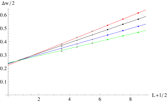
Figure 2: Plots of $\frac{\Delta w}{2}=\frac{1}{2}\left(w_{\infty}(L+1)-w_{\infty}(L)+\frac{1}{2}\log\left(1+\frac{1}{L}\right)\right)$ obtained with method 1) as a function of $L+\frac{1}{2}$ at $S=0.4$ and $b=0.36$ (red), $b=0.362$ (black), $b=0.365$ (blue) and $b=0.368$ (green). Error bars are not visible in the plot. The straight lines show linear fits through the corresponding data points. Only points $6<L+\frac{1}{2}<9$ are used in the fits. The string tension values obtained from these fits are collected in Table 1.

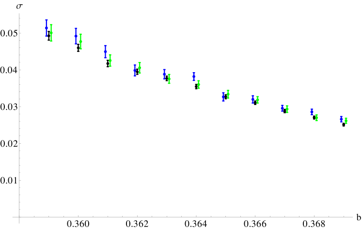
Figure 3: Plots of the string tension values of Table 1: method 1) in black, method 2a) in green, method 2b) in blue. $b$-values for 2a) and 2b) are slightly shifted to opposite sides of the true $b$-value for visibility.

4.3 Continuum limit

A scale length in lattice units denoted by $\xi_{c}(b)$ is used to carry out extrapolations to the continuum limit. It is defined at $N=\infty$ using a three-loop calculation of the $\beta$-function for the lattice coupling. The coefficients are written as ${\bar{\beta}_{i}}$, $i=0,1,2$.

$$\bar{\beta}_{0} =\frac{\beta_{0}}{N}=\frac{11}{48\pi^{2}}\,,$$ (4.7)

$$\bar{\beta}_{1} =\frac{\beta_{1}}{N^{2}}=\frac{34}{3(16\pi^{2})^{2}}\,,$$ (4.8)

$$\bar{\beta}_{2} =\lim_{N\to\infty}\frac{\beta_{2}}{N^{3}}\approx-3.12211\times 10^{-5}\,.$$ (4.9)

Integrating the RG flow, we define:

$$\xi_{c}(b)=0.26\left(\frac{\bar{\beta}_{1}}{\bar{\beta}_{0}^{2}}+\frac{b_{I}(b)}{\bar{\beta}_{0}}\right)^{-\frac{\bar{\beta}_{1}}{2\bar{\beta}_{0}^{2}}}\,\exp\left[\frac{b_{I}(b)}{2\bar{\beta}_{0}}\right]\,\exp\left[\frac{\bar{\beta}_{2}}{2\bar{\beta}_{0}^{2}b_{I}(b)}\right]\,.$$ (4.10)

Above we have replaced the gauge coupling $b$ by $b_{I}(b)$,

$$b_{I}(b)=\lim_{N,V\to\infty}b\,W_{N}(L=1,b,S=0,V)\,,$$ (4.11)

a substitution known as tadpole improvement. In practice this substitution gets one much more rapidly into the asymptotic regime where truncated perturbation theory reasonably accurately describes the RG flow. The improved infinite-$N$ coupling constant $b_{I}(b)$ is defined without smearing.

The definition of $\xi_{c}(b)$ is taken to match with [19]. We only added a numerical prefactor to make $\xi_{c}(b)\approx L_{c}(b)$, where $L_{c}(b)$ is given in [15]. This approximation is good to 10-15% in our range of couplings and would become exact at $b=\infty$. It is well known that direct continuum extrapolations are subject to large systematic errors since one is too far from a truly asymptotic regime. There are many prescriptions for what to use. We do not have a particular opinion about which one is best. Our objective in this paper is not to obtain the highest accuracy possible with our data. We preferred to choose a reasonable existing prescription to facilitate comparison with other numerical work on closely related topics. The net consequence of this is that numerical results for the continuum limit are substantially less accurate than numerical results at finite lattice spacing. The work of different groups may sometimes be compared only in the continuum limit, and sometimes also at finite lattice spacing. It is possible that one ends up with a statistically significant discrepancy at finite lattice spacing but no statistically significant discrepancy in the continuum limit. This will be the situation for our determination of the string tension, but this remark has to be qualified by the comment that one needs to add the observation that on the lattice one should get identical numbers for the string tension extracted from the two point function of Polyakov loops and that extracted from rectangular loops.

We separately carry out two two-parameter fits of the relation between the string tension $\sigma(b)$ and $\xi_{c}(b)$. The two pairs of parameters are denoted by $d_{0}$, $d_{1}$ and $f_{0}$, $f_{1}$:

$$\sigma(b)=\frac{d_{0}}{\xi_{c}(b)^{2}}+\frac{d_{1}}{\xi_{c}(b)^{4}}$$ (4.12)

and

$$\frac{1}{\xi_{c}(b)^{2}}=f_{0}^{-1}\sigma(b)+f_{1}\sigma(b)^{2}\,.$$ (4.13)

We use ranges $0.359\leq b\leq 0.369$ (range A) and $0.362\leq b\leq 0.367$ (range B). We also use the limited $b$ range (B) since we have observed increasing $\chi^{2}$’s for the infinite-$N,V$ extrapolations using method 2a) for $b\leq 0.361$. This was mentioned in Sec. 4.1. Another reason is that finite-volume effects increase with increasing $b$. This reason only applies to method 1).

Results for $d_{0}$ and $f_{0}$ using the $\sigma(b)$ values in Table 1 are given in Table 3. Plots of the corresponding fit functions (4.12) and (4.13) are shown in Fig. 4.

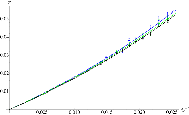
Figure 4: Plots of $\sigma$ as a function of $\xi_{c}^{-2}$: method 1) in black, method 2a) in green, method 2b) in blue, together with fit functions (4.12) (solid lines) and (4.13) (dashed lines). The fits are obtained using $0.359\leq b\leq 0.369$ (range A); results for $d_{0}$ and $f_{0}$ are given in Table 3.

The difference between the two fits is a simple indicator of systematic errors induced by the truncation of the perturbative series. For all continuum extrapolations $d_{0}<f_{0}$. These particular systematic deviations are of the same order as the statistical errors.

The result of Allton et al. [19] is $\sigma\xi_{c}^{2}\to 1.85$ in our notation with a statistical error of 1% and a systematic error of 16% on the continuum result. Their numbers were extracted from Polyakov loops which are substantially longer than one side of our rectangular loops. Apparently, the physical length of string that came into their calculations allows for a substantially more accurate determination of the string tension. The systematic errors are dominated by the extrapolation to continuum and their relative size is roughly the same for us. Although we work at somewhat higher $b$-values, this has little impact on the extrapolation. Our $b$’s are still too far from the full set-on of perturbative asymptotics.

Setting $\bar{\beta}_{2}=0$ in the expression for $\xi_{c}(b)$ (cf. Eq. (4.10)) results in an increase of about 26% for $d_{0}$, and an increase of about 29% for $f_{0}$, cf. Table 4 and Fig. 5. This number is too large to commit to a precise estimate of the systematical error. We could be optimistic and assume that the next term in perturbation theory would make a smaller correction but it is hard to tell.

Figure 5: Same as Fig. 4 for $\bar{\beta}_{2}=0$ in $\xi_{c}(b)$ (cf. Eq. (4.10)). Fit results are given in Table 4.

Later we shall find some rough estimates of the effective coupling constant $\frac{g^{2}N}{4\pi}$ at our smearing levels and it would come out to be of order unity. The definition of $\xi_{c}(b)$ is at zero smearing, so these effective couplings are not directly relevant. Nonetheless, the large systematic error coming from truncating perturbation theory comes as no surprise.

In summary, we find that the infinite-$N$ continuum string tension is given by

$$\lim_{b\to\infty}\sigma(b)\xi^{2}_{c}(b)=1.6(1)(3)\,.$$ (4.14)

The first error is statistical and the second systematic. The systematic error is more of a guess than a well founded estimate. Our central number is 2-3 standard deviations smaller than that of [19]. In terms of $\Lambda_{\overline{MS}}$, this translates to:

$$\sigma/\Lambda_{\overline{MS}}^{2}=3.4(2)(6)\,.$$ (4.15)

A previous estimate for the string tension at infinite $N$ extracted from rectangular loops has been given in [20]. Expressed in terms of our variables it is $\sigma\xi_{c}^{2}|_{b_{I}=0.182}=2.2(3)$. The results of [20] are claimed to be compatible with [19] at infinite $N$. These results were obtained working at $N=37,47,59$ on a $6^{4}$ lattice at small values $b=0.345,0.348,0.350$ assuming large-$N$ reduction and including folded loops in the analysis.

While writing up this paper a new study [21] appeared which also deals with rectangular Wilson loops with the objective to test a new method of full twisted large-$N$ reduction [22]. This successful test is carried out on the physical value of the string tension. These authors obtain $\frac{\sigma}{\Lambda_{{\overline{M}S}^{2}}}=3.63(3)$ (statistical error) at $N=\infty$ in the continuum if they apply the continuum extrapolation method of [19]. This number is fully consistent with ours and has very small errors by comparison. The number in [19] is $\frac{\sigma}{\Lambda_{{\overline{M}S}^{2}}}=3.95(3)(64)$ at $N=\infty$ in the continuum.

There seems to be a disagreement at the statistical level between [19] and our result which agrees with that of [21]. The result of [20] seems to side with that of [19], but has too large errors to be sure. The systematic error is too big to claim evidence for a difference between the string tension extracted from Wilson loops and that extracted from Polyakov loop correlators by [19] in the continuum limit. Such a difference would be very difficult to accept at the theoretical level. Given the differences between these various simulations the case for a real discrepancy between the Wilson loop string tension and the Polyakov correlator string tension at the lattice level is not worrying so far. If one ignores smearing, these two string tensions ought to be equal already at the lattice level. It might be of interest to settle this in future work.

4.4 String tension at finite $N$

We now determine the string tension in lattice units at finite $N$. Extrapolating to infinite $N$ this would show how the string tension in lattice units converges to its infinite-$N$ limit. We do this in order to get a feel about the commutativity of the limits $N\to\infty$ and UV-cutoff $\to\infty$.

We determine the string tension $\sigma_{N}$ at fixed $b$, $S$, $V$ and $N$, by fitting $c_{2,N}$ and $\sigma_{N}$ in

$$\frac{1}{2}\left(w_{N}(L+1)-w_{N}(L)+\frac{1}{2}\log\left(1+\frac{1}{L}\right)\right)=\sigma_{N}\left(L+\frac{1}{2}\right)+\frac{c_{2,N}}{2}$$ (4.16)

to $6\leq L\leq 9$ square loop data. We use data obtained on volumes $V=24^{4}$, $18^{4}$, $14^{4}$, $12^{4}$ for $N=7$, $11$, $19$, $29$, respectively, as detailed earlier. We already mentioned in Sec. 4.1 that for these cases we believe that finite-volume effects are negligible. For $N=7$, $11$, $19$ we use $S=0.52$, and for $N=29$ we use $S=0.4$. As before, there is no dependence on $S$ within statistical errors and the errors decrease with increasing $S$ (cf. Sec. 4.5 below).

Figure 6 shows plots of the finite-$N$ string tensions as a function of $b$ together with the infinite-$N$ result obtained from $w_{\infty}$ by method 1) in Sec. 4.2. For fixed $b\leq 0.367$ the results for the string tension at finite $N$ are well described by

$$\sigma_{N}(b)=\sigma_{\infty}(b)+\frac{h(b)}{N^{2}}\,.$$ (4.17)

Results for $\sigma_{N}$ and fit parameters $\sigma_{\infty}$, $h$ are given in Table 5. The infinite-$N$ string tension obtained in this manner is in good agreement with our previous results in Table 1. Those results were determined from $w_{\infty}$. We see that $h(b)\sim 10\sigma_{\infty}(b)$. A relative variation of order $\frac{10}{N^{2}}$ may seem large. At fixed lattice coupling $b$ one would need to go to $N$ values of order 20 to be able to credibly extrapolate to infinite $N$.

It will become clear later on, in section 4.6, that the large coefficient of the $\frac{1}{N^{2}}$ term is replaced by a much smaller one when one looks at $\sigma$ not as a function of $b$, but as a function of $b$ times the plaquette average. The plaquette average also has a finite $N$ correction and the fact that it works in the manner described is relatively well know, as mentioned in Sec. 4.6.

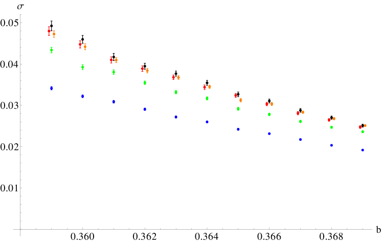
Figure 6: Plots of the finite-$N$ string tension $\sigma_{N}(b)$ from square loops for $N=7$ (blue), $N=11$ (green), $N=19$ (orange), $N=29$ (red) together with the infinite-$N$ result (black) obtained by method 1), cf. Table 1. $b$-values for $N=19$ and $N=29$ are slightly shifted in $b$ in the plot for visibility.

4.5 Smearing dependence

Figures 7 and 8 show plots of $w_{N}$ as a function of $L$ for two different smearing levels $S=0.28$ and $S=0.52$, for $N=11$, $V=18^{4}$, $b=0.365$. Also shown are plots of the individual terms $w_{N}$ is composed of (cf. Eq. (5.2)). The variation in $\sigma_{N}$ is about 1.9%, of the order of the statistical errors (1.2% for $S=0.52$, 2.6% for $S=0.28$). $c_{2}$ and $c_{1}$ exhibit larger variation.

These figures allow us to see the relative sizes of the various contributions to the Wilson loop at fixed smearing and how these relative contributions change when smearing is changed. For a small amount of smearing the negative of the logarithm of the Wilson loop is larger (see the red data points and the total fit drawn as a black curve). This mainly reflects the larger size of the perimeter term whose contribution is larger than that of the area term. The log-term also makes a sizable contribution, smaller than that of the area term. The smallest contribution comes from the shape-dependent constant. The logarithmic dependence on smearing of the latter has small numerical impact.

Wilson loops larger than their critical size smoothly merge with their behavior for small sizes. One can imagine how all terms except the area one do this. The area term has to morph into something else. A likely candidate is a term going as the area squared (for planar loops). This term comes from the dimension four condensate which would enter in an expansion in loop size small relative to the extent of smearing. For a square loop of side $l$ and smearing $s$, one gets from one gluon exchange $w_{N}=\frac{g^{2}N}{4\pi}\frac{1}{128\pi}\frac{l^{4}}{s^{2}}$. So, we only need something like $l^{2}/s<20$ for this approximation to become relevant.

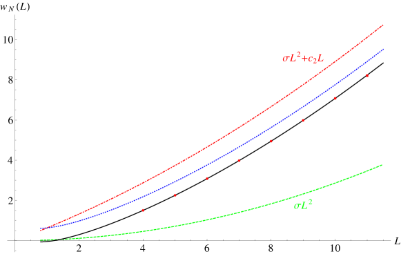
Figure 7: Plot of $w_{N}(L)$ for $N=11$ on $V=18^{4}$ at $b=0.365$ and $S=0.28$ (red points, error bars are not visible), together with analytic functions $\sigma L^{2}$ (green, dashed), $\sigma L^{2}+c_{2}L$ (red, dotdashed), $\sigma L^{2}+c_{2}L-\frac{1}{2}\log L$ (blue, dotted), and $\sigma L^{2}+c_{2}L-\frac{1}{2}\log L+c_{1}$ (black, solid). The fit parameters used to plot the analytic functions were obtained from the data at $6\leq L\leq 9$. They are $\sigma=0.02863$, $c_{2}=0.6041$, $c_{1}=-0.6788$.

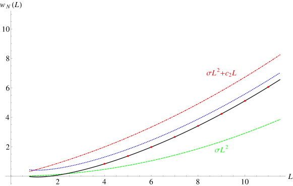
Figure 8: Same as Fig. 7 for $S=0.52$. Here, $\sigma=0.02916$, $c_{2}=0.3813$, $c_{1}=-0.4624$.

The level of smearing in lattice units was varied in a large enough range to contain levels of smearing in physical scales that are relevant both to the proximity of the large-$N$ transition and to testing whether there is a dependence on smearing in the continuum limit. We see that the string tension does not depend on the smearing parameter within statistical errors. These errors decrease rapidly with increasing $S$ (cf. Fig. 9 for an example).

We can check whether the expected continuum divergences as $s\to 0$ indeed are detected. On the lattice there will be no divergence as $S\to 0$, since the lattice spacing regulates all divergences, regardless of whether they come from the Lagrangian or from the observable. With a reasonable amount of smearing one detects a window where the amount of smearing exceeds the lattice spacing influence but is still small enough to exhibit the behavior that would have caused a divergence in the continuum. Fig. 10 shows that the $c_{2}$ coefficient of the perimeter term increases linearly with $\frac{1}{\sqrt{S}}$, $c_{2}=c_{2}^{(0)}+c_{2}^{(1)}/\sqrt{S}$ in this window. Similarly, Fig. 11 shows that the $S$-dependence of the $L$-independent term $c_{1}$ is consistent with a $\log(S)$ $S\to 0$ divergence: $c_{1}=-0.2538+0.3278\log S$.

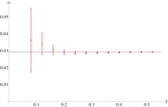
Figure 9: String tension as a function of the smearing parameter $S$ for $N=11$, $b=0.365$, $V=18^{4}$. $\sigma$ is determined using square loops with $6\leq L\leq 9$. The horizontal black line corresponds to $\sigma(S=0.52)=0.02916$.

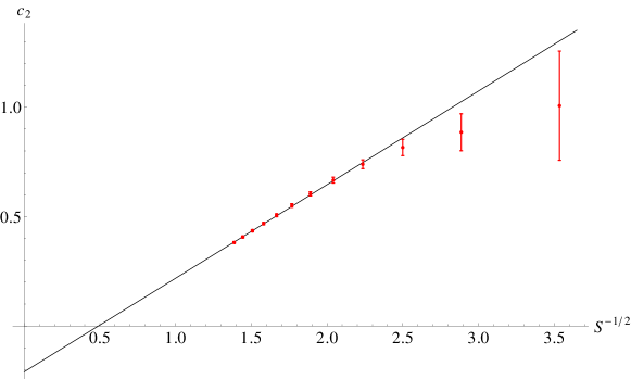
Figure 10: Perimeter coefficient $c_{2}$ (determined from square loops with $6\leq L\leq 9$) as a function of the smearing parameter $S$ for $N=11$, $b=0.365$, $V=18^{4}$. The straight black line shows the fit $c_{2}=-0.2097+0.4279/\sqrt{S}$.

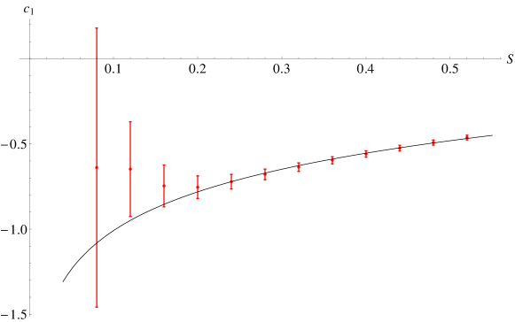
Figure 11: $L$-independent constant $c_{1}$ (determined using square loops with $6\leq L\leq 9$) as a function of the smearing parameter $S$ for $N=11$, $b=0.365$, $V=18^{4}$. The black line shows the fit $c_{1}=-0.2538+0.3278\log S$.

4.6 Continuum limit for finite $N$

Most of the relatively large finite-$N$ corrections to the string tension get absorbed when considered at fixed improved coupling $b_{I}(b,N)$ rather than fixed $b$. Figure 12 makes this clear. $b_{I}(b,N)$ is determined by the unsmeared plaquette averages at the corresponding finite value of $N$. Tadpole improvement simultaneously improves the approach to continuum and to infinite $N$. Looking at $\sigma_{N}(b_{I})$ instead of $\sigma_{N}(b)$ gives a better indication for the speed of large-$N$ convergence in the continuum.

We extrapolate to the continuum at finite $N$ using Eqs. (4.12, 4.13) with the finite-$N$ values for $\xi_{c}$, $\beta_{2}$ and $b_{I}$. Once we employ the improved coupling scheme, we no longer observe a significant $N$-dependence in $d_{0}(N)$ or $f_{0}(N)$. This is shown in Fig. 13. This feature of tadpole improvement [19] was first seen in the context of Polyakov loop correlators and is reviewed in [23].

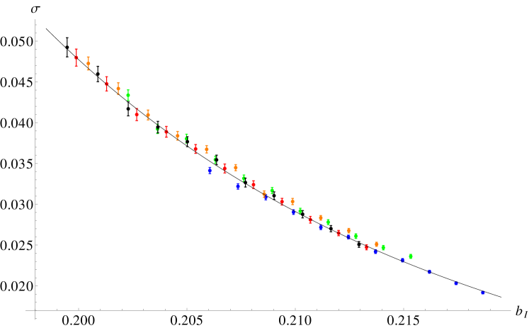
Figure 12: Same data as in Figure 6 now plotted as a function of the improved coupling $b_{I}$. The solid line shows the result of the continuum extrapolation [method 1) & range A in Table 3] for the infinite-$N$ string tension, $\sigma(b)=1.50/\xi_{c}(b)^{2}+21/\xi_{c}(b)^{4}$, cf. Eq. (4.12).

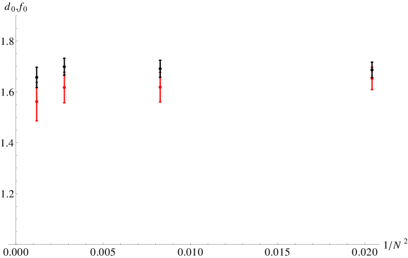
Figure 13: Plot of $d_{0}(N)$ (red) and $f_{0}(N)$ (black) determined from finite-$N$ versions of Eqs. (4.12, 4.13) fitted in the range $0.359\leq b\leq 0.367$.

4.7 Tree-level continuum perturbation theory

We calculated the expectation value of a rectangular $l_{1}\times l_{2}$ loop in tree-level continuum perturbation theory. Diagrammatically, this gives a one-loop integral with a tree-level smeared propagator. By “tree-level” we refer to the absence of propagator and vertex radiative corrections.

We parameterize a general closed curve $\operatorname{\cal C}$ by $x(u)$ with $x(0)=x(1)$ and $\dot{x}(u)\equiv\partial_{u}x(u)$). To leading order in $g^{2}$, $w_{N}^{\text{PT}}=-\log W_{N}$ is given by

$$w_{N}^{\text{PT}}(\operatorname{\cal C},s) =\frac{1}{2}g^{2}C_{2}\int_{0}^{1}du_{1}\int_{0}^{1}du_{2}\,D(x(u_{1})-x(u_{2});s)\delta_{\mu\nu}\dot{x}_{\mu}(u_{1})\dot{x}_{\nu}(u_{2})\,,$$ (4.18)

$$D(x;s) =\int\frac{d^{4}p}{(2\pi)^{4}}\,e^{ip\cdot x}\frac{1}{p^{2}}\,e^{-2sp^{2}}\,.$$ (4.19)

$C_{2}$ is the quadratic Casimir invariant given by $C_{2}^{\text{fund}}=\frac{N^{2}-1}{2N}$ in the fundamental representation. We first take a derivative w.r.t. $s$ to bring the integrand into Gaussian form,

$$\partial_{s}D(x;s)=-\frac{1}{2^{5}\pi^{2}s^{2}}e^{-\frac{x^{2}}{8s}}\,.$$ (4.20)

Integrating around a rectangular $l_{1}\times l_{2}$ loop over $u_{1,2}$ then produces error functions. Next, we integrate over $s$, using $D(x,s)\to 0$ as $s\to\infty$.

$$w_{N}^{\text{PT}}(l_{1},l_{2},s)=-\int_{s}^{\infty}ds^{\prime}\,\partial_{s^{\prime}}w_{N}^{\text{PT}}(l_{1},l_{2},s^{\prime})\,$$ (4.21)

leads to

$$w_{N}^{\text{PT}}(l_{1},l_{2},s)=\frac{g^{2}C_{2}}{2}\,h\left(\frac{s}{l_{1}^{2}},\frac{s}{l_{2}^{2}}\right)$$ (4.22)

with

$$h\left(\frac{s}{l_{1}^{2}},\frac{s}{l_{2}^{2}}\right)=\frac{2}{\pi^{2}}\int_{0}^{\frac{l_{1}}{\sqrt{8s}}}dz\left(1-e^{-(l_{2}/l_{1})^{2}z^{2}}\right)\left(\frac{\sqrt{\pi}}{2}\operatorname{erf}(z)+\frac{1}{2z}\left(e^{-z^{2}}-1\right)\right)+l_{1}\leftrightarrow l_{2}\,.$$ (4.23)

For $s/l_{i}^{2}$ small, we get

$$h\left(\frac{s}{l_{1}^{2}},\frac{s}{l_{2}^{2}}\right)=\frac{1}{(2\pi)^{\frac{3}{2}}}\left(\frac{l_{1}+l_{2}}{\sqrt{s}}\right)+\frac{1}{\pi^{2}}\log\left(\frac{s}{l_{1}l_{2}}\right)+h_{0}\left(\frac{l_{2}}{l_{1}}\right)+\mathcal{O}\left(\frac{s}{l_{i}^{2}}\right)\,.$$ (4.24)

$h_{0}(l_{2}/l_{1})=h_{0}(l_{1}/l_{2})$ has the following integral representation:

$$h_{0}\left(\frac{l_{2}}{l_{1}}\right)=\frac{2}{\pi^{2}}\int_{0}^{1}dz\left(2-e^{-(l_{2}/l_{1})^{2}z^{2}}-e^{-(l_{1}/l_{2})^{2}z^{2}}\right)\left(\frac{\sqrt{\pi}}{2}\operatorname{erf}(z)+\frac{1}{2z}\left(e^{-z^{2}}-1\right)\right)$$

$$\quad+\frac{2}{\pi^{2}}\int_{1}^{\infty}dz\left[\left(2-e^{-(l_{2}/l_{1})^{2}z^{2}}-e^{-(l_{1}/l_{2})^{2}z^{2}}\right)\left(\frac{\sqrt{\pi}}{2}\operatorname{erf}(z)+\frac{1}{2z}\left(e^{-z^{2}}-1\right)\right)-\sqrt{\pi}+\frac{1}{z}\right]$$

$$\quad+\frac{3}{\pi^{2}}\log 2-\frac{2}{\pi^{\frac{3}{2}}}\,.$$ (4.25)

Beyond the perimeter divergence a loop with kinks will have logarithmic singularities as $s\to 0$. At each kink we denote by $\gamma_{i}$ the angle between the tangents. The well known expression is:

$$\log(W_{N})_{\rm corners}=-\sum_{i}\frac{g^{2}C_{2}({\rm fundamental})}{4\pi^{2}}(\gamma_{i}\cot\gamma_{i}-1)\log\left(\frac{{\rm Length}(C)}{\sqrt{s}}\right)\,.$$ (4.26)

Exactly backtracking segments of $\operatorname{\cal C}$ should cancel out for any $s\neq 0$. Nonetheless, the coefficient of the $\log(s)$ divergence above blows up as $\gamma_{i}\to\pi$. The limits $s\to 0$ and $\gamma_{i}\to\pi$ do not commute. This is not a surprise, because when a finite loop segment becomes exactly backtracking the perimeter changes discontinuously, affecting already the leading term in the $s\to 0$ asymptotic series.

Note the appearance of the logarithm of the perimeter at leading order in perturbation theory. There is a well known fundamental difference between the perimeter divergence and the logarithmic one in higher orders of perturbation theory [24]: While the perimeter divergence maintains its tree-level dependence on the loop to all orders, the corner divergence does not because it corresponds to a kink-angle dependent anomalous dimension. Were we to choose to define the overall scale as the square root of the minimal area, this term would add a shape dependence to the logarithm of the Wilson loop. The logarithm of the perimeter comes in from the integral over gluon exchanges where the gluon connects point on the opposing sides of the corner. When both endpoints are close to the corner the propagator is conformal approximately and this generates a logarithm of the distance along each side of the angle. For a very dilated loop having a finite number of separated kinks, one expects to leave the conformal regime before any other kink is encountered. This would replace the logarithm of the perimeter in the corner divergence term by $\log\frac{1}{\Lambda}$. We assumed that $s$ stays fixed, of the order $\frac{1}{\Lambda^{2}}$. As we mentioned already, there are corner terms going as $\log^{\kappa}s$ at higher order which sum up to $\log(\log s)$ in the LLA.

4.7.1 Perimeter coefficient

We have seen numerically that there is a term in the logarithm of the smeared Wilson loops which is proportional to the perimeter and diverging as $s^{-\frac{1}{2}}$ for $s\to 0$. This is a local divergence on the loop and therefore ought to be calculable in perturbation theory. One expects no $\log(s)$ divergent contributions to the perimeter term at all orders in perturbation theory.

From Eqs. (4.22, 4.24) we get the following tree-level formula for the perimeter term for a square $l\times l$ loop:

$$\frac{g^{2}C_{2}}{2}\,\frac{1}{(2\pi)^{\frac{3}{2}}}\,\frac{2l}{\sqrt{s}}\,.$$ (4.27)

For example, at $b=0.365$ and $N=11$, we have obtained $c_{2}=-0.2097+0.4279/\sqrt{S}$ (cf. Fig. 10). Matching the coefficient of the $L/\sqrt{S}$ term with tree-level PT would require $\frac{g^{2}N}{4\pi}\approx 1.08$. This is an indication for the order of magnitude for an effective running coupling at this level of smearing.

4.7.2 Coefficient of $\log(s)$

The corner divergence at tree level in Eq. (4.24) provides a $\log(s)$ term in $w_{N}$:

$$\frac{g^{2}C_{2}}{2}\,\frac{1}{\pi^{2}}\log s\,.$$ (4.28)

For example, at $b=0.365$ and $N=11$, we obtained $0.3278$ for the coefficient of the $\log S$ term in $w_{N}$ (cf. Fig. 11). Matching the numerical result with PT would require $\frac{g^{2}N}{4\pi}\approx 1.03$. This is consistent with the perimeter term determination of $\frac{g^{2}N}{4\pi}$.

5 $L\times 2L$ loops – shape dependence

We turn now to a study of the shape dependence of the size-independent term in $w_{N}$ and compare it with the effective-string prediction. In general, a shape-dependent parameter characterizing a loop $\operatorname{\cal C}$ is a dimensionless number describing $\operatorname{\cal C}$ which is invariant under a scaling or an $\mathbb{R}^{4}$ space-time symmetry applied to $\operatorname{\cal C}$. For rectangular $L_{1}\times L_{2}$ loops it is convenient to introduce the modular invariant shape parameter

$$\zeta=\frac{L_{1}}{L_{2}}+\frac{L_{2}}{L_{1}}\,.$$ (5.1)

This $\zeta$ should not be confused with the $\zeta$-function that will appear later.

The accuracy we now need does not permit taking the $N\to\infty$ limit. We restrict our attention to the $N=7,11$ data. We shall see that the numbers we compute are identical within errors for $N=7$ and $N=11$, indicating that it is unlikely that they will change in a substantial manner in the $N=\infty$ limit.

At fixed $b$, $S$, $V$, and fixed finite $N$, we expect

$$w_{N}(L_{1},L_{2})+\frac{1}{4}\log L_{1}L_{2}=c_{1,N}(\zeta)+c_{2,N}\frac{L_{1}+L_{2}}{2}+\sigma_{N}L_{1}L_{2}+\mathcal{O}\left(\frac{1}{\sigma_{N}L_{1}L_{2}}\right)\,.$$ (5.2)

Here, the arguments $b$, $S$, $V$ are omitted and the single length scale $L$ of squares is replaced by $L_{1}$ and $L_{2}$ for rectangles.

We extracted the lattice string tension from square $L\times L$ loops at fixed finite $N$, $b$, $S$, $V$ in Sec. 4.4. We determined $\sigma_{N}$ by fitting the data using Eq. (4.16) with fit parameters $\sigma_{N}$ and $c_{2,N}$. After subtracting area and perimeter terms, we fitted $w_{N}(L,L)+\frac{1}{4}\log L^{2}-\sigma_{N}L^{2}-c_{2,N}L$ to a constant. This constant is now denoted by $c_{1,N}(\zeta=2)$.

We now analyze the results obtained for a sequence of rectangular loops at the same $b$, $S$, $V$, $N$ with $L_{2}=2L_{1}$, i.e., $\zeta=\frac{5}{2}$ fixed. Using the results for $\sigma_{N}$ and $c_{2,N}$ obtained from square loops above, we determine $c_{1,N}(\zeta=\frac{5}{2})$ by fitting $w_{N}(L,2L)+\frac{1}{4}\log\left(2L^{2}\right)-\sigma_{N}2L^{2}-c_{2,N}\frac{3}{2}L$ to a constant. Figures 14 and 15 show plots of $c_{1,N}(2.5)-c_{1,N}(2)$ as a function of $b$ for $N=7$ and $N=11$. The $L$-ranges used for fitting $c_{1,N}$ are $6\leq L\leq 10$ for square loops and $4\leq L\leq 7$ for $L\times 2L$ loops. The smallest loop areas included in each set are therefore 36 and 32, respectively, putting them close to the large-$N$ phase transition point.

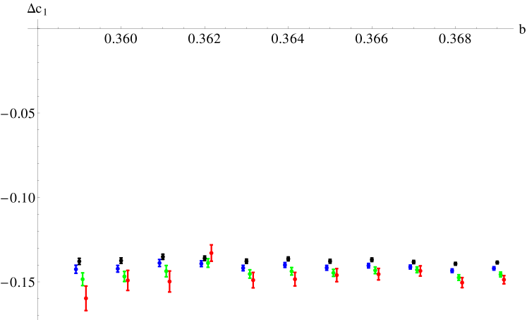
Figure 14: Plot of $c_{1,N}(2.5)-c_{1,N}(2)$ for $N=7$ (on $V=24^{4}$) as a function of $b$ for $S=0.2$ (red), $S=0.28$ (green) $S=0.4$ (blue), and $S=0.52$ (black).

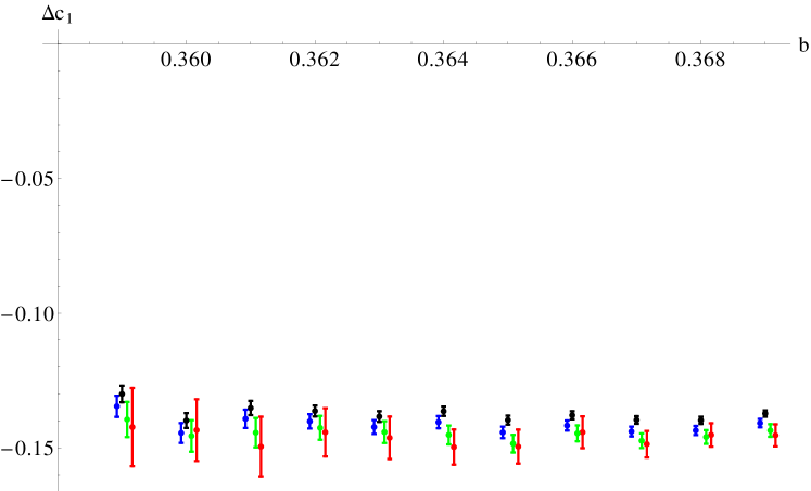
Figure 15: Plot of $c_{1,N}(2.5)-c_{1,N}(2)$ for $N=11$ (on $V=18^{4}$) as a function of $b$ for $S=0.2$ (red), $S=0.28$ (green) $S=0.4$ (blue), and $S=0.52$ (black).

The effective-string prediction for $c_{1}(2.5)-c_{1}(2)$ is

$$\frac{1}{2}\log\left(\frac{\eta(2i)\eta(i/2)}{\eta(i)^{2}}\right)\approx-0.08664\,,$$ (5.3)

where $\eta(x)$ is the eta-function. We find that the effective-string prediction is smaller than the observed values (cf. Figs. 14, 15) by a factor of about 1.5 to 1.7. Within statistical errors, our results for $c_{1,N}(2.5)-c_{1,N}(2)$ do not depend on $b$, $S$, or $N$.

6 Almost square loops

We use sequences of almost square loops with sides $L_{1}=L$, $L_{2}=L\pm 1$ to cross check our results for the string tension and the shape dependence of $c_{1,N}$. For these loops, the shape-parameter $\zeta$ changes with $L$ and is given by

$$\zeta=\frac{L\pm 1}{L}+\frac{L}{L\pm 1}=2+\frac{1}{L^{2}}\mp\frac{1}{L^{3}}+\mathcal{O}\left(L^{-4}\right)\,.$$ (6.1)

6.1 String tension

Expanding $c_{1,N}(\zeta)$ around $\zeta=2$, we obtain from Eq. (4.16)

$$\frac{1}{2}\left(w_{N}(L,L+1)-w_{N}(L,L-1)+\frac{1}{4}\log\frac{L+1}{L-1}\right)=\sigma_{N}L+\frac{c_{2,N}}{2}+\ldots$$ (6.2)

We dropped corrections of order $\frac{1}{L^{3}}$ from the $\zeta$ expansion and $\frac{1}{\sigma L^{3}}$ from the effective-string expansion.

Similarly to the procedure for square loops, we first take $\lim_{N,V\to\infty}w_{N}$ and then determine the infinite-$N$ string tension from $w_{\infty}$. Here, we use only method 1), i.e., we compute the limit $w_{\infty}$ from data at $N=7$, $11$, $19$, $29$ on volumes $V=24^{4}$, $18^{4}$, $14^{4}$, $12^{4}$, respectively (for $N=7$ we use $V=24^{4}$ for $b\geq 0.365$ and $V=20^{4}$ for $b\leq 0.364$).

To determine $\sigma$ and $c_{2}$ from Eq. (6.2) (at infinite $N$) we use loops of sizes $6\times 7$, $7\times 8$, $8\times 9$.

The results for the infinite-$N$ string tension $\sigma(b)$ determined in this manner agree very well with those obtained from square loops, cf. Table 6 and Fig. 16.

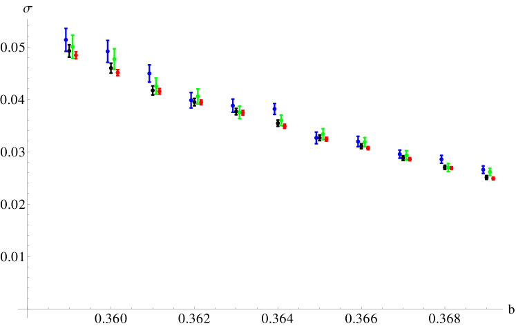
Figure 16: Plots of the infinite-$N$ string tension obtained from rectangular $L\times L\pm 1$ loops (cf. Table 6) in red, together with results from square loops in black, blue, green (identical to plots in Fig. 3).

6.2 Shape dependence

Using square and almost square loops, we can study the shape dependence of $c_{1,N}(\zeta)$. From Eq. (5.2), ignoring corrections of order $1/L^{4}$ and $1/\sigma L^{4}$, we obtain

$$\Delta w_{N}(L)\equiv w_{N}(L,L)-\frac{1}{2}w_{N}(L,L+1)-\frac{1}{2}w_{N}(L,L-1)=-\frac{c_{1,N}^{\prime}(2)}{L^{2}}-\frac{1}{8L^{2}}+\ldots$$ (6.3)

In the first term on the r.h.s $c_{1,N}^{\prime}(\zeta)\equiv\frac{dc_{1,N}(\zeta)}{d\zeta}$. The second term on the r.h.s. results from the $\frac{1}{4}\log L_{1}L_{2}$ term in Eq. (5.2). To determine $c_{1,N}^{\prime}(2)$ we multiply $\Delta w_{N}$ by $L^{2}$ and fit to a constant in the range $5\leq L\leq 8$ (for an example see Fig. 17). Note the constancy of $c_{1,N}^{\prime}(2)$ as a function the gauge coupling. This indicates that the number we extracted from the data is already in the continuum limit within quite small errors.

In $\Delta w_{N}(L)$, both the shape-dependent constant $c_{1}(\zeta)$ and the $\frac{1}{4}\log L_{1}L_{2}$ term result in terms of the order $1/L^{2}$ and only their sum can be determined. From the effective-string prediction, we would expect $L^{2}\Delta w_{N}(L)\to 0.0372764$ for large $L$ taking into account both contributions. This produces the value $c_{1}^{\prime}(2)\approx-0.162276$.

The effective string model produces asymptotic predictions for both $c_{1}(\zeta)$ and $\frac{1}{4}\log L_{1}L_{2}$ from the determinant of Gaussian fluctuations. One may refer to this prediction as a 1-loop prediction of effective string theory, to distinguish it from subleading contributions, suppressed by powers of the area in units of the string tension.

Our numerical results for $L^{2}\Delta w_{N}(L)$ deviate significantly from the asymptotic string prediction (cf. Fig. 17). There is no upfront indication in the data that subleading terms in the asymptotic series given by effective string theory play any role since there is no dependence on the gauge coupling. Such a dependence would have to appear if the data were better described, say, by including a subleading correction. This subleading correction would go as one over the area in string tension units and would depend on the gauge coupling $b$ through the lattice string tension $\sigma$. Here, we cannot decide whether the deviation originates from the shape-dependent constant $c_{1}(\zeta)$ or the $\log L_{1}L_{2}$ term. However, when we determine the string tension from square loops, our results seem to be consistent with a $\log L$ term as predicted by the string model (see also Sec. 7). This indicates that $c_{1}(\zeta)$ is responsible for the deviations.

Taking into account the $\frac{1}{8L^{2}}$ term coming from the $\log$ (i.e., we assume that the coefficient of the $\log L_{1}L_{2}$ term in $w_{N}$ is correctly determined by the string model), our results for $c_{1}^{\prime}$ exceed the asymptotic string prediction by a factor of about 1.6 to 1.8. Since $c_{1}(2.5)$ in the string prediction is very well approximated (to an accuracy of 2%) by an expansion around $\zeta=2$ to linear order, this discrepancy is consistent with the discrepancy of $c_{1}(2.5)-c_{1}(2)$ observed in Sec. 5. Our result here is also in agreement within errors with [21] who independently report a deviation from string theory.

We do not observe any significant dependence on $b$, $S$ or $N$ (cf. Fig. 18 for results at $S=0.4$).

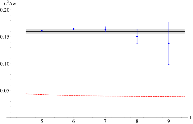
Figure 17: Plot of $L^{2}\Delta w_{N}(L)$ for $N=11$, $V=18^{4}$, $b=0.365$, $S=0.4$ (blue points), result of fit to a constant (black solid line, error estimate indicated by the gray band), and string prediction (red dashed line).

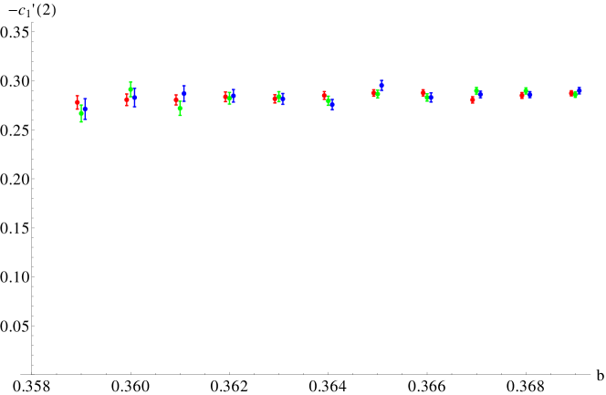
Figure 18: Plot of $-c_{1,N}^{\prime}(2)$ as a function of $b$ at $S=0.4$ for $N=7$ on $V=20^{4}$ (red), $N=11$ on $V=18^{4}$ (green), and $N=19$ on $V=14^{4}$ (blue). (We define $c_{1}^{\prime}(2)$ as $c_{1}^{\prime}(2)=-L^{2}\Delta w_{N}-\frac{1}{8}$; the effective-string prediction is $c_{1}^{\prime}(2)\approx-0.162276$.)

There is a question we shall address later on: Is it consistent within effective string theory to keep only the leading term? This question is meaningful in the sense that the theory predicts a correction of known, universal strength. The expansion in inverse area produces a series which likely is divergent. If a subleading correction is larger or equal to the leading one, one would conclude that either further terms are needed or, one is outside the reach of the asymptotic series in inverse size altogether and no further terms would be of any help. Then the fact that the data showed no dependence on the gauge coupling $b$ would have to be explained in some other way, unrelated to effective string theory. To prepare for this eventuality we need to address two questions first. Do we have numerical evidence for the logarithm of area term? What would perturbation theory have to say about the Wilson loops in this range?

6.2.1 Perturbation theory

Extracting the shape-dependent terms from square $l\times l$ and almost square $l\times(l\pm\delta l)$ loops similar to $\Delta w_{N}$ defined in Eq. (6.3) in Sec. 4.7, we obtain

$$\Delta w_{N}^{\text{PT}}(l,\delta l,s)=w_{N}^{\text{PT}}(l,l,s)-\frac{1}{2}w_{N}^{\text{PT}}(l,l+\delta l,s)-\frac{1}{2}w_{N}^{\text{PT}}(l,l-\delta l,s)$$

$$\quad=\frac{g^{2}C_{2}}{2}\left(\frac{1}{2\pi^{2}}\log\left(1-\frac{\delta l^{2}}{l^{2}}\right)+h_{0}(1)-\frac{1}{2}h_{0}\left(1+\frac{\delta l}{l}\right)-\frac{1}{2}h_{0}\left(1-\frac{\delta l}{l}\right)+\mathcal{O}\left(\frac{s}{l^{2}}\right)\right)$$

$$\quad=\frac{g^{2}C_{2}}{2}\left(\left(-\frac{1}{2}h_{0}^{\prime\prime}(1)-\frac{1}{2\pi^{2}}\right)\left(\frac{\delta l}{l}\right)^{2}+\mathcal{O}\left(\frac{s}{l^{2}},\frac{\delta l^{4}}{l^{4}}\right)\right)\,.$$ (6.4)

Numerically, we found $h_{0}^{\prime\prime}(1)\approx-0.260476$ and thus

$$\Delta w_{N}^{\text{PT}}(l,\delta l,s)=\frac{g^{2}C_{2}}{2}\left(0.0795774\left(\frac{\delta l}{l}\right)^{2}+\mathcal{O}\left(\frac{s}{l^{2}},\frac{\delta l^{4}}{l^{4}}\right)\right)\,.$$ (6.5)

We have seen that some terms which diverge at zero smearing, and clearly are outside the reach of effective string theory, enter in the logarithm of the smeared Wilson loop in a simple additive manner. The case of shape dependence is more complicated and shall be discussed later on, when we look at possible explanations for the deviation of the shape dependence we measure from the asymptotic prediction of effective string theory.

7 All loops: validation of the log-term

So far we have assumed that all our Wilson loops had a prefactor given by $(\rm Area)^{\frac{1}{4}}$. We mentioned that attempts to carry out our fits without this term produced substantially lower quality fits. We now would like to determine whether the power $\frac{1}{4}$ really is selected by our numbers. To do this we need an amount of data and accuracy which does not allow us to consider separately different loop shapes or take the infinite-$N$ limit. We do global fits to all our data at two values of $N$.

At fixed $N$, $b$, $S$, we fit square $L\times L$, almost square $L\times(L+1)$, and rectangular $L\times(2L)$ loops to

$$w_{N}(L_{1},L_{2})=\sigma L_{1}L_{2}+c_{3}\log\left(L_{1}L_{2}\right)+c_{2}\frac{L_{1}+L_{2}}{2}+c_{1}+c_{4}\left(\frac{L_{1}}{L_{2}}+\frac{L_{2}}{L_{1}}-2\right)\,.$$ (7.1)

Some results are given in Tables 7 and 8. Going to smaller loops, $\chi^{2}/N_{\text{dof}}$ starts to increase significantly. Tables 7 and 8 tell us that the value $\frac{1}{4}$ for the exponent of the area is consistent with the data.

7.1 $\log(\text{Area})$ versus shape dependence

We have seen now that one prediction coming from the determinant in the effective string description works close to the large-$N$ transition in the eigenvalues and the other does not.

These two predictions are somewhat different even within effective string theory. The determinant of the small fluctuations of the spanning surface around the minimal area one is most conveniently evaluated using $\zeta$-function regularization. The determinant itself is ill defined and $\zeta$-function regularization provides one way to extract finite universal features. Only such features are conceivably relevant to Wilson loops.

Within $\zeta$-function regularization one has the option to make a decision about how to treat the directions perpendicular to the surface which now are fields in the two-dimensional theory on the world-sheet. This description is supposed to be geometrical without introducing any scale. It is convenient to enforce this by thinking in terms of two-dimensional gravity. Then, it is natural to view the fields as half-densities [25]. With this convention, the power of the area is a regulated number of degrees of freedom, coming from $\zeta(0;D)$ where $D$ is the fluctuation operator. The rest of the determinant is just a function of the shape parameter $\zeta$ and comes from the derivative $d\zeta(w;D)/dw|_{w=0}$, reflecting the eigenvalues of $D$ more directly.

$\zeta(0,D)$ has additive contributions coming from each kink in our planar curve $\operatorname{\cal C}$:

$$\sum_{i}\frac{\pi^{2}-\theta_{i}^{2}}{24\pi\theta_{i}}\,.$$ (7.2)

Here, the $0\leq\theta_{i}\leq 2\pi$ are the angles at each kink measured by an arc contained in the interior of $\operatorname{\cal C}$. For a rectangular loop, summing over the two orthogonal directions to the surface produces the factor $\frac{1}{4}$. For a backtracking loop the corner term would blow up. For a smeared Wilson loop, a backtracking segment makes no contribution.

$\zeta$-function regularization extracts the universal predictions. It is natural to use a two-dimensional lattice regularization for the effective string instead. This is so because in the strong coupling expansion of the lattice gauge theory one can identify contributions given by the exponent of the area of a spanning surface made out of tiles that can be labeled by two fields depending on two coordinates on a square world-sheet lattice. It is easy to numerically determine the asymptotic expansion in $L$ of the fluctuation determinant for a square loop, assuming the two fields to be continuous:

$$\log\prod_{n=1}^{L-1}\prod_{m=1}^{L-1}\left(2-\cos\frac{n\pi}{L}-\cos\frac{m\pi}{L}\right)\sim 0.4731L^{2}-0.37645L-\frac{1}{2}\log L-0.09039+\ldots$$ (7.3)

We see that there is an area term, a perimeter term and a constant but they are absorbed into the physical area law, the well defined perimeter and constant terms in the case of smeared loops. It is just as easy to do this for a rectangular loop. It is possible to derive the asymptotic expansion for rectangular loops by analytical means too. Below we reproduce part of Eq. (4.20) from [26]:

$$\log\prod_{n=1}^{N-1}\prod_{m=1}^{M-1}\left(4-2\cos\frac{n\pi}{L}-2\cos\frac{m\pi}{L}\right) \sim MN\frac{4G}{\pi}-(M+N)\log(1+\sqrt{2})$$

$$\quad-\frac{1}{4}\log MN+...$$ (7.4)

Here, $G=1-1/3^{2}+1/5^{2}...$ is Catalan’s constant. The universal results using $\zeta$-function regularization are reproduced. The derivation of [26] shows that the logarithmic term comes from modes that vary little (have small wave numbers) in one of the two directions parallel to the sides of the rectangle. These modes are the ones most affected by the Dirichlet boundary conditions.

Looking at the exact expression for the determinant for finite integer $(M,N)$ we find that the asymptotic expansion truncated after the constant term provides estimates for the logarithm of the determinant at relative accuracy 0.014% for $M,N\geq 5$ and 0.0065% for $M,N\geq 6$. The largest deviation in both sets is at $M=N$. For loops at fixed aspect ratio of 2, $M=2N$, the relative accuracy is $0.024\%$ for $N=4$ and $0.0012\%$ for $N=8$. In this simple case, quite small loops are very well described by the asymptotic series without any terms that vanish as $M,N\to\infty$.

One cannot tell a priori what if anything is left from this numerical observation when one looks at real Wilson loops. If this held also for real Wilson loops we would expect to see a shape dependence independent on the gauge coupling $b$ for loops as small as we looked at. But, then, the number should have agreed with the asymptotic prediction of the determinant.

7.2 Possible explanations of the deviation of the shape dependent constant from the prediction of asymptotic effective string theory

One employs effective string theory under the hypothesis that once the ultimate asymptotic regime is entered, it will take complete control of the shape dependence of the functionals $W(\operatorname{\cal C})$. Specifically, in the kind of asymptotic expansion in dilatation that we are considering (which is different from looking at the separation dependence of the interquark force for example) one has, as $\rho\to\infty$, the following behavior for a dilated loop $\rho\operatorname{\cal C}$:

$$\log(W(\rho\operatorname{\cal C})) \sim-\sigma\rho^{2}{\rm Area}_{\rm min}(\operatorname{\cal C})+\Gamma_{P}\;\rho\,{\rm Length}(\operatorname{\cal C})+\Gamma_{1}(\operatorname{\cal C})\log(\rho)+\Gamma_{2}(\operatorname{\cal C})$$

$$\quad+\Gamma_{K}(\operatorname{\cal C})+\Gamma_{3}(\operatorname{\cal C})/\rho^{2}+\Gamma_{4}(\operatorname{\cal C})/\rho^{3}+\Gamma_{5}(\operatorname{\cal C})/\rho^{4}+{\cal O}(1/\rho^{5})\,.$$ (7.5)

One can think about $\rho$ and $\operatorname{\cal C}$ as follows: Let the minimal area with some $\operatorname{\cal C}^{\prime}$ as boundary be unique. Multiply this area by the string tension and get a pure number. Scale $\operatorname{\cal C}^{\prime}$ by an amount that makes this number equal to 1 and call the so obtained curve $\operatorname{\cal C}$. Choose a parametrization of this curve $\operatorname{\cal C}$ by a $x_{\mu}(\tau)$ with a choice of $\tau$ such that $\dot{x}^{2}=1$. Then, the information contained in $\operatorname{\cal C}$ is equivalent to the information contained in the set of all global $\rm O(4)$ invariants one can construct out of the function $\dot{x}_{\mu}$. $\tau$ goes once round $\operatorname{\cal C}$. Note that with this convention, the perimeter of $\rho\operatorname{\cal C}$ depends on $\operatorname{\cal C}$.

$\operatorname{\cal C}$ is allowed to have kinks. $\sigma$ is dimensional and has nothing to do with effective string theory, except that $\sigma>0$. The perimeter coefficient $\Gamma_{P}$ is a non-universal number independent of $\operatorname{\cal C}$. $\Gamma_{1}(\operatorname{\cal C})$, $\Gamma_{2}(\operatorname{\cal C})$, $\Gamma_{3}(\operatorname{\cal C})$, and $\Gamma_{5}(\operatorname{\cal C})$ are scale-invariant functions of $\operatorname{\cal C}$ and universal. $\Gamma_{4}(\operatorname{\cal C})$ is a scale-invariant function of $\operatorname{\cal C}$ with one non-universal overall constant multiplicative factor.

$$\Gamma_{K}(\operatorname{\cal C})=\sum_{\rm kinks}F(\dot{x}_{+}\cdot\dot{x}_{-}|_{\rm kink})\,.$$ (7.6)

A crucial assumption is that the non-universal function $F()$ is independent of $\operatorname{\cal C}$, and that its argument is given by the discontinuity in the tangent of $\operatorname{\cal C}$ at the kinks. Without this assumption one cannot separate $\Gamma_{2}(\operatorname{\cal C})$ from $\Gamma_{K}(\operatorname{\cal C})$. With this assumption the $\Gamma_{K}$ term can be eliminated by comparing loops $\operatorname{\cal C}_{1}$ and $\operatorname{\cal C}_{2}$ which have the same set of kinks. In this case, effective string theory makes a testable prediction for $\Gamma_{2}(\operatorname{\cal C}_{1})-\Gamma_{2}(\operatorname{\cal C}_{2})$.

The presence of the terms $\Gamma_{P}$ and $\Gamma_{K}$ in Eq. (7.2) can be motivated in four-dimensional Yang-Mills field theory. The Wilson loop has perimeter and corner ultraviolet divergences whose removal will introduce some ad-hoc parameters one could not expect effective string theory to know about. According to this logic, Wilson loops in three-dimensional Yang-Mills theory with continuous gauge groups would not require a $\Gamma_{K}$ term. From the effective string theory point of view there is no motivation for such distinction between four and three dimensions.

Equation (7.2) is tested in only a limited manner on rectangular loops. $\Gamma_{K}$ is a fixed constant in this set of loops. Since we encountered a deviation at order $\rho^{0}$ at the level of the universality of $\Gamma_{2}(\operatorname{\cal C})$, we could suspect that the problem has to do with the presence of kinks. Since any kink can be rounded, the requirement on the size of $\rho$ needed in order to justify keeping only the leading terms up to and including $\Gamma_{2}$ in the asymptotic expansion in large $\rho$ involves the local radius of curvature of $\operatorname{\cal C}$, ${\cal R}$. For a kink-free $\operatorname{\cal C}$, parametrically described by a $x(\tau)$, we have

$${\cal R}(\tau)=\frac{({\dot{x}}^{2})^{\frac{3}{2}}}{\sqrt{{\dot{x}}^{2}{\ddot{x}}^{2}-({\dot{x}}\cdot{\ddot{x}})^{2}}}\,.$$ (7.7)

${\cal R}$ is invariant under re-parameterizations of the boundary and under $\operatorname{\cal C}\to\rho\operatorname{\cal C}$ it scales like $\rho$. With the choice ${\dot{x}}^{2}=1$, we have ${\cal R}=1/|{\ddot{x}}|$, which endows the parameter $\tau$ with the same dimension as that of $x$. Effectively, in the presence of a single “almost” kink, the Wilson loop depends on two hugely disparate scales. There exists a field-theoretical definition of the smeared Wilson loop, and we know from experience that observables depending on very disparate scales are hard to calculate. It could be though that the effective string theory provides a framework which is so different from field theory that this experience is irrelevant.

We now proceed to ask a simpler question: does effective string theory tell us that the subleading corrections to the shape dependence are so large that we had no right to compare the data to the leading asymptotic prediction? Had we obtained agreement, we probably would not have raised this question, like in many previous studies of the interquark force [8], which produced agreement in the leading term in the asymptotic expansion relevant to that case.

Within the premise of effective string theory we are working, there is no substantial difference for rectangular loops between something as simple as $Z_{2}$ gauge theory in three Euclidean dimensions and $\operatorname{SU}(\infty)$ pure gauge theory in four Euclidean dimensions. Consequentially one has ready examples in the recent literature [27] for how to include subleading terms.

In the next subsection we carry out this exercise on our data.

After that we come back to discuss at a more intuitive level possible differences between $Z_{2}$ three-dimensional gauge theory on the lattice, which is exactly dual to the three-dimensional Ising model and hence has a field-theoretical continuum description built around the Wilson-Fisher fixed point, and four-dimensional planar $\operatorname{SU}(N)$ gauge theory.

7.3 Subleading terms in effective string theory

The subleading corrections that have been looked at in detail come in at orders $\frac{1}{\rho^{2}},\frac{1}{\rho^{3}},\frac{1}{\rho^{4}}$ corresponding, respectively, to a bulk, a boundary and another bulk correction. Corner corrections have not been discussed in the effective string literature, as far as we know. The two bulk corrections have universal coefficients, known functions of the shape parameter $\zeta$. The boundary term has an adjustable coefficient. There exists an unresolved discrepancy in the coefficient of $\rho^{-2}$: there are two candidates, denoted as ${\cal L}_{2}(u)$ and $\hat{\cal L}_{2}(u)$ differing by a $u$-independent number, where $u+u^{-1}=\zeta$. In the plots we show the contributions of each candidate, hoping that one is correct. We have not rechecked the calculations of the coefficients by ourselves. We could add these terms as corrections to the effective string theory partition function and then take the logarithm or directly to the logarithm. Since the numbers differ for our values of loop area, we show both cases.

We show different forms of contributions up to order $\rho^{-2}$ in three examples in figures 19, 20, and 21. The black points/lines represent the numerical data in all figures. With

$$\tilde{w}(L_{1},L_{2})\equiv w(L_{1},L_{2})+\frac{1}{4}\log L_{1}L_{2}-\sigma L_{1}L_{2}-c_{2}\frac{L_{1}+L_{2}}{2}-c_{1}(\zeta=2)$$ (7.8)

for rectangular $L_{1}\times L_{2}$ loops, the colored lines pertaining to the effective string description are defined as follows:

• Red: $\rho^{0}$-term coming from the determinant, $\tilde{w}(L_{1},L_{2})=\frac{1}{2}\log\left(\eta(iu)\eta(i/u)\eta^{-2}(i)\right)$.

• Solid green: $\tilde{w}(L_{1},L_{2})=\frac{1}{2}\log\left(\eta(iu)\eta(i/u)\eta^{-2}(i)\right)-\log\left(1+\frac{{\cal L}_{2}(u)}{\sigma L_{1}L_{2}}\right)$ is used to include the term of order $\rho^{-2}$.

• Dashed green: $\tilde{w}(L_{1},L_{2})=\frac{1}{2}\log\left(\eta(iu)\eta(i/u)\eta^{-2}(i)\right)-\log\left(1+\frac{\hat{\cal L}_{2}(u)}{\sigma L_{1}L_{2}}\right)$ is used to include the term of order $\rho^{-2}$.

• Solid orange: $\tilde{w}(L_{1},L_{2})=\frac{1}{2}\log\left(\eta(iu)\eta(i/u)\eta^{-2}(i)\right)-\frac{{\cal L}_{2}(u)}{\sigma L_{1}L_{2}}$ is used to include the term of order $\rho^{-2}$.

• Dashed orange: $\tilde{w}(L_{1},L_{2})=\frac{1}{2}\log\left(\eta(iu)\eta(i/u)\eta^{-2}(i)\right)-\frac{\hat{\cal L}_{2}(u)}{\sigma L_{1}L_{2}}$ is used to include the term of order $\rho^{-2}$.

For the subleading terms, we use $\sigma=0.02916$ (as obtained from square loops for $N=11$ at $b=0.365$, cf. Table 5). Note that

$$\Delta\tilde{w}(L)\equiv\tilde{w}(L,L)-\frac{1}{2}\tilde{w}(L,L+1)-\frac{1}{2}\tilde{w}(L,L-1)=\Delta w(L)-\frac{1}{8}\log\left(1-L^{-2}\right)\,.$$ (7.9)

The adjustable order $\rho^{-3}$ term is not shown in the figures because we would have to fit its coefficient. We also ignore the order $\rho^{-4}$ term, although it would produce distinguishable numbers on the plots

In $\tilde{w}(L,2L)-\tilde{w}(L,L)$ (cf. Fig. 20), square loops are subtracted from rectangular loops which have an area twice as large. Therefore, the effective string predictions with ${\cal L}_{2}$ and $\hat{\cal L}_{2}$ differ at next-to-leading order.

It is quite clear that if we wanted to add the missing $\mathcal{O}\left(\rho^{-3}\right)$ boundary term, we could get agreement between theory and a few more data points, for smaller loops. One may conclude then that effective string theory applies to our data. That the boundary term would scale correctly is an automatic consequence of the $b$-independence of the data.

Alternatively, one may simply conclude that for our loops effective string theory makes no definite prediction for the shape dependence. We face a standard situation with asymptotic series: adding too many terms is a bad idea and so is having too few. How one looks at the data becomes quite subjective.

Be that as it may, since the main focus of our work is to determine which predictions of effective string theory hold close enough to the infinite-$N$ phase transition and therefore could come in when one tried to match onto perturbation theory, we are left where we were before carrying out this exercise: beyond the area term we can use with some confidence also the logarithmic term. Employing effective string prescribed terms of higher order in $\rho^{-1}$ becomes questionable.

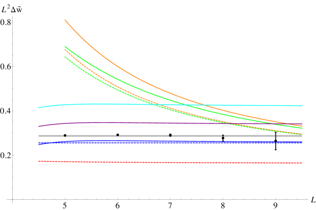
Figure 19: Plot of $L^{2}\Delta\tilde{w}(L)$ (black points) for $N=11$, $V=18^{4}$, $b=0.365$, $S=0.4$ together with the result of a fit to a constant (thin dark-grey line, error estimate indicated by the light-gray band). The various colored lines show estimates obtained from effective string theory (green, orange) and tree-level perturbation theory (blue, purple, cyan) as described in Secs. 7.3 and 7.4.

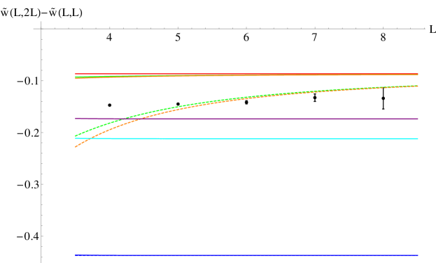
Figure 20: Plot of $\tilde{w}(L,2L)-\tilde{w}(L,L)$ (black points) for $N=11$, $V=18^{4}$, $b=0.365$, $S=0.4$. Numerical results for $\tilde{w}$ are obtained by subtracting area-, perimeter-, and constant-term (with coefficients determined from square loop data) from measured $w(L_{1},L_{2})+\frac{1}{4}\log(L_{1}L_{2})$.

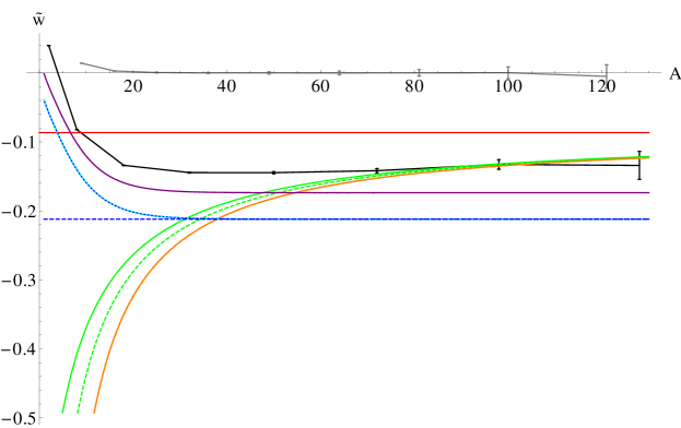
Figure 21: Plot of $\tilde{w}(L,2L)$ (black) and $\tilde{w}(L,L)$ (gray) as a function of the area $A$ for $N=11$, $V=18^{4}$, $b=0.365$, $S=0.4$. Since $\tilde{w}(L,L)$ is zero within errors (except for the smallest loops), $\tilde{w}(L,2L)$ can be viewed as a reasonable estimate for $\tilde{w}(\sqrt{2A},\sqrt{A/2})-\tilde{w}(\sqrt{A},\sqrt{A})$. The various colored lines show effective-string and perturbative predictions for this difference as a function of the area $A$.

7.4 Rough estimates in perturbative field theory

We now take an orthogonal view: we try to see how the data could be described by field theory in perturbation theory. Just as with the effective string description, we are most likely outside the proper reach of this expansion too. It is clear however that one cannot dispense with the area term, albeit that it is not predictable by field-theoretical perturbation theory. Regarding the term logarithmic in the area coming from effective string theory, we choose to eliminate it. Perturbation theory will come with its own logarithms and there is no objective way to mix them with logarithms coming from effective string theory. The relevant lines in the figures 19, 20, 21 are defined below.

• Solid blue: $\tilde{w}(l_{1},l_{2},s)=w^{\text{PT}}(l_{1},l_{2},s)-\frac{g^{2}C_{2}}{2}\frac{1}{(2\pi)^{\frac{3}{2}}}\left(\frac{l_{1}+l_{2}}{\sqrt{s}}\right)$ (cf. Eqs. (4.22, 4.24)).
  Note that shifting $\tilde{w}$ by a ($l_{1}/l_{2}$-independent) constant has no effect on the observables we are considering here.

• Dashed blue: leading term (in the large-$l_{i}/\sqrt{s}$ expansion) of the above.

• Cyan: $\tilde{w}(l_{1},l_{2},s)=w^{\text{PT}}(l_{1},l_{2},s)-\frac{g^{2}C_{2}}{2}\left(\frac{1}{(2\pi)^{\frac{3}{2}}}\left(\frac{l_{1}+l_{2}}{\sqrt{s}}\right)+\frac{1}{\pi^{2}}\log\left(\frac{s}{l_{1}l_{2}}\right)\right)$.
  Replacing the $\log(s/l_{1}l_{2})$-term in $w^{\text{PT}}(l_{1},l_{2},s)$ by $\log(s\Lambda^{2})$, this term would no longer contribute to the shape dependence. Then the leading order contribution is determined by $h_{0}(l_{2}/l_{1})$ only (cf. Eq. (4.24)).

• Purple: $\tilde{w}_{N}=w_{N}^{\text{PT}}(l_{1},l_{2},s)-\frac{g^{2}C_{2}}{2}\left(\frac{1}{(2\pi)^{\frac{3}{2}}}\left(\frac{l_{1}+l_{2}}{\sqrt{s}}\right)+\frac{1}{\pi^{2}}\log\left(\frac{s}{(l_{1}+l_{2})^{2}}\right)\right)$.
  This corresponds to the replacement $\log(s/(l_{1}+l_{2})^{2})\to\log(s\Lambda^{2})$ in $w^{\text{PT}}(l_{1},l_{2},s)$.

For our perturbative estimates shown in Figs. 19, 20, 21, we set the coupling constant to $\frac{g^{2}N}{4\pi}=1.03$, the value that we obtained from the coefficient of the $\log(s)$-term for $b=0.365$, $N=11$ (cf. Sec. 4.7.2).

Our information from perturbation theory is clearly too limited at this stage to draw any concrete conclusions. As far as we went, it seems to work just as well or as badly as effective string theory.

7.5 Suggestions for further research of the shape dependence

Summarizing the situation so far, it seems that for moderate sizes loops one observes a continuum shape dependence which might be explained by perturbation theory and might upon extension to much larger loops transit to another value given by effective string theory.

Taking into account what we know about nonabelian four-dimensional theories, we think that the issue of shape dependence deserves further study, albeit somewhat tangential to our own long-range project.

Further numerical checks could be made focusing on the specific issue of shape dependence. An interesting set of Wilson loops amenable to study on hypercubic lattices have $\theta_{i}$ angles equal to $\frac{3\pi}{2}$. The loop is not convex and for such angles the difference between the effective-string shape dependence and the field-theoretical one is enhanced. Physically, in perturbation theory gluons exchanged between different segments of the loop will predominantly choose to travel through the “outside” for an obtuse corner angle. On the other hand, surfaces of effective string theory fluctuate above the “inside” of the loop, convex or not. In this context it would be also of interest to consider self-intersecting loops given by fitting a figure of 8 onto a hypercubic lattice.

We suggest that the shape dependence of planar Wilson loops presents an interesting case for testing the limitations of the effective string approach. We know that a high-energy scattering event in QCD produces after degradation into the IR a pattern of jets that is an imprint of perturbation theory.

• Could it be that even an asymptotically dilated Wilson loop with kinks in Euclidean space would have elements of shape dependence that are determined by the field theory at short distances and which do not get washed out at large distances?

• Were that the case, is the effective string theory framework flexible enough to allow the inclusion of specific kink terms that can be adjusted to exactly reproduce the angle dependence of the anomalous dimensions associated with kinks?

7.6 How much should one expect 3D lattice $Z_{2}$ gauge theory to teach us about $\operatorname{SU}(\infty)$ 4D pure Yang-Mills theory?

In 3D gauge theories with continuous groups there are no corner singularities. The perimeter term is only logarithmically divergent. The renormalization properties of the Wilson loop operators are significantly different. We emphasized several features of the corner singularities in 4D gauge theory. They have no analogues in 3D. The corner singularities play a role in determining the shape dependence of Wilson loops in 4D. Further, the case of discrete gauge groups in 3D is substantially distinct from the case of continuous groups.

One place one can compare the two theories would be on the lattice. For 4D Yang-Mills theory one has well defined loop equations. These equations have a formal continuum limit in which loops with kinks play a crucial role. The Ising model, which is dual in three dimensions to the $Z_{2}$ gauge model also has a lattice loop equation in terms of a “barbed wire” loop boundary [28]. The equation is very different from the four-dimensional lattice loop equation for Yang-Mills.

These equations look stringy, and it has been the folklore that they would lead to an exact dual string description. It seems plausible that if such an exact dual description exists, the appropriate effective string would bear some closeness to it, say in terms of the correct massless degrees of freedom one should use. This may make no difference at leading order, but at higher order what is local on the world sheet in one description might be non-local in another. The string dual of the Ising model seems not to have a tunable string coupling constant, while the string dual of $\operatorname{SU}(N)$ gauge theory seems to have one, which can be set to zero by taking $N$ to infinity. There seems to be no analogous freedom and limit in the 3D case. Even if handles are exponentially suppressed for the three-dimensional Ising case, there is no control on this and no way we know of to actually estimate their numerical values; once one works at loop sizes and accuracies sensitive to higher order terms in $\rho$ than the leading one it is difficult to asses how much of a match between data and theory one ought to expect. In the large-$N$ limit of $\operatorname{SU}(N)$ gauge theory there is a credible argument that at least one does not have to worry about handle corrections.

We urge caution in drawing conclusions from 3D $Z_{2}$ lattice gauge theory about 4D Yang-Mills theory. The results of applying effective string theory to the three-dimensional Ising model are quite impressive in themselves, without necessarily being relevant in detail to four-dimensional gauge theories of the type we have in Nature at a rather fundamental level.

8 Conclusions

A stringy parametrization for rectangular Wilson loops holds relatively well all the way down to the large-$N$ transition point. Notably, the scale dependence of the $\Gamma_{1}(\operatorname{\cal C})\log(\rho)$-term is consistent with a correct interpretation of the number of degrees of freedom living on the worldsheet in the Nambu-Goto case. However, when one gets to the subleading level of the dependence on purely shape-dependent parameters, the situation is less clear.

We are specifically interested in the large-$N$ limit of four-dimensional $\operatorname{SU}(N)$ pure gauge theories and in contours with corner singularities. It could be that there is another effective string theory prescription that takes into account the corners in a special way. It would describe the large-$\rho$ asymptotics of Wilson loops with corners in some different manner. To make the Wilson loops we are interested in well defined in the continuum limit, one would need to either use smeared loops, or an alternative method, to eliminate the ultraviolet divergences inherent in the field-theoretical definition of the observables under consideration. Effective string theory is supposed to apply to continuum observables and to be free of ultraviolet cutoff effects. After applying constraints resulting from spacetime invariance in four dimensions, all ambiguities still present are supposedly parameterizable by terms local on the worldsheet, on the boundary and at the corners. These extra terms make contributions to the Wilson loops that are suppressed by non-negative powers of the inverse area measured in units of the string tension. An effective string theory different from the one employed here might use a different set of fields, or allow different kinds of additions representing corners, or both.

So far, it seems possible to try to roughly match rectangular loops across the large-$N$ phase transition. We need to perform more checks on the short scales side of the transition to see if one can ultimately turn this into a credible estimate of the ratio $\sigma/\Lambda_{\overline{MS}}^{2}$.

Our results might be taken as an indication to consider other observables that admit an effective string representation. Much work has been done on the two-point correlation function of Polyakov loops. Here, there are no corner divergences to worry about. So far one has not established an analogue of the large-$N$ phase transition in Wilson loops in this case, but we believe this to be possible. So, maybe focusing on Polyakov loop correlations would provide a way to temporarily circumvent the issue of dependence on loop shape in the presence of kinks. A more esoteric option is to use surface operators where the regularization of the operator presents less difficulty [29].

In any case, the issue of shape dependence is seen not to be a numerical impediment to obtaining a reasonably accurate estimate of $\sigma/\Lambda^{2}$ by analytical means. Only refinements at a later stage might have to take this issue into account. Nonetheless, at a deeper level a full understanding of the interplay between field-theoretical properties of kinks and a good effective string description of large loops promises to be illuminating.

9 Acknowledgments

HN would like to thank Ofer Aharony for a very useful e-mail exchange and the authors of  [21] for a friendly heads-up regarding the posting of their preprint. HN thanks the GGI Institute for hosting the 2010 workshop on “Large-$N$ gauge theories”. Several discussions with participants in this workshop were very helpful. Our research is supported in part by the DOE under grant number DE-FG02-01ER41165.

10 Tables

Method 1)
$b$	$\sigma$
0.359	0.0492(12)
0.360	0.04597(94)
0.361	0.04170(86)
0.362	0.03946(71)
0.363	0.03767(61)
0.364	0.03544(58)
0.365	0.03266(55)
0.366	0.03105(47)
0.367	0.02878(45)
0.368	0.02701(38)
0.369	0.02508(36)

Method 2a)
$b$	$\sigma$
0.359	0.0500(22)
0.360	0.0477(20)
0.361	0.0425(15)
0.362	0.0405(14)
0.363	0.0375(12)
0.364	0.0360(10)
0.365	0.0334(10)
0.366	0.03183(87)
0.367	0.02931(89)
0.368	0.02696(76)
0.369	0.02614(69)

Method 2b)
$b$	$\sigma$
0.359	0.0514(22)
0.360	0.0492(21)
0.361	0.0449(16)
0.362	0.0398(15)
0.363	0.0388(13)
0.364	0.0382(10)
0.365	0.0326(11)
0.366	0.03195(98)
0.367	0.02954(77)
0.368	0.02854(76)
0.369	0.02657(72)

Table 1: Results for the infinite-$N$ string tension $\sigma$ at $S=0.4$.

Method 1)
$b$	$\sigma$
0.359	0.0487(22)
0.360	0.0456(17)
0.361	0.0430(16)
0.362	0.0400(13)
0.363	0.0373(11)
0.364	0.03577(99)
0.365	0.03252(84)
0.366	0.03106(73)
0.367	0.02842(77)
0.368	0.02713(62)
0.369	0.02462(57)

Method 2a)
$b$	$\sigma$
0.359	0.0480(39)
0.360	0.0486(33)
0.361	0.0434(28)
0.362	0.0434(24)
0.363	0.0363(21)
0.364	0.0347(17)
0.365	0.0331(17)
0.366	0.0314(14)
0.367	0.0288(15)
0.368	0.0271(13)
0.369	0.0255(11)

Method 2b)
$b$	$\sigma$
0.359	0.0543(40)
0.360	0.0504(37)
0.361	0.0466(30)
0.362	0.0393(25)
0.363	0.0377(22)
0.364	0.0412(18)
0.365	0.0318(19)
0.366	0.0317(16)
0.367	0.0295(14)
0.368	0.0289(13)
0.369	0.0261(12)

Table 2: Results for the infinite-$N$ string tension $\sigma$ at $S=0.28$.

method & range	$d_{0}$	$\chi^{2}/N_{\text{dof}}$	$f_{0}$	$\chi^{2}/N_{\text{dof}}$
1) & A	1.50(6)	0.51	1.62(3)	0.63
2a) & A	1.55(11)	0.24	1.66(6)	0.25
2b) & A	1.55(11)	0.80	1.68(5)	0.79
1) & B	1.55(14)	0.42	1.65(7)	0.46
2a) & B	1.64(27)	0.14	1.71(16)	0.14
2b) & B	1.54(26)	1.56	1.68(13)	1.59

Table 3: Extrapolation to the continuum using $\sigma$ from Table 1.

fit	$d_{0}$	$\chi^{2}/N_{\text{dof}}$	$f_{0}$	$\chi^{2}/N_{\text{dof}}$
1) & A	1.89(8)	0.51	2.10(3)	0.69
2a) & A	1.94(15)	0.24	2.15(7)	0.26
2b) & A	1.95(16)	0.80	2.18(7)	0.79
1) & B	1.95(19)	0.42	2.13(9)	0.48
2a) & B	2.07(37)	0.14	2.20(19)	0.15
2b) & B	1.93(36)	1.56	2.17(15)	1.61

Table 4: Continuum extrapolations using $\xi_{c}(b)$ with setting $\bar{\beta}_{2}=0$ in (4.10).

$b$	$\sigma_{7}$	$\sigma_{11}$	$\sigma_{19}$	$\sigma_{29}$	$\sigma_{\infty}$	$h$	$\chi^{2}/N_{\text{dof}}$
0.359	0.03413(38)	0.04337(65)	0.04726(79)	0.0480(11)	0.04927(60)	-0.741(37)	0.14
0.360	0.03219(33)	0.03924(57)	0.04418(71)	0.04476(87)	0.04533(53)	-0.647(33)	1.3
0.361	0.03086(32)	0.03804(54)	0.04094(60)	0.04100(74)	0.04231(46)	-0.559(29)	0.64
0.362	0.02904(28)	0.03546(43)	0.03839(52)	0.03888(66)	0.03974(39)	-0.524(26)	0.09
0.363	0.02717(27)	0.03318(40)	0.03673(44)	0.03678(54)	0.03772(34)	-0.518(23)	0.91
0.364	0.02599(23)	0.03168(37)	0.03449(37)	0.03438(55)	0.03551(31)	-0.466(20)	0.81
0.365	0.02420(24)	0.02916(35)	0.03124(40)	0.03240(47)	0.03259(30)	-0.412(20)	0.35
0.366	0.02314(21)	0.02781(30)	0.03033(38)	0.03032(41)	0.03108(27)	-0.389(18)	0.68
0.367	0.02172(18)	0.02610(28)	0.02834(28)	0.02810(40)	0.02906(23)	-0.359(16)	1.3
0.368	0.02032(17)	0.02468(27)	0.02677(28)	0.02647(32)	0.02740(21)	-0.345(14)	2.2
0.369	0.01917(16)	0.02361(25)	0.02510(25)	0.02473(31)	0.02582(20)	-0.322(13)	4.6

Table 5: String tension at finite $N=7$, $11$, $19$, $29$, and results of the corresponding extrapolations to infinite $N$ (obtained by fitting $\sigma_{\infty}$ and $h$ in Eq. (4.17)).

Method 1) for rect.
$b$	$\sigma$
0.359	0.04842(66)
0.360	0.04510(56)
0.361	0.04153(53)
0.362	0.03943(43)
0.363	0.03744(45)
0.364	0.03486(39)
0.365	0.03239(37)
0.366	0.03068(29)
0.367	0.02858(29)
0.368	0.02688(25)
0.369	0.02489(26)

Table 6: Results for the infinite-$N$ string tension $\sigma$ from rectangular $L\times L\pm 1$ loops at $S=0.4$.

$b$	$S$	$\sigma$	$c_{3}$	$c_{2}$	$c_{1}$	$c_{4}$	$\chi^{2}/N_{\text{dof}}$
0.365	0.52	0.02462(29)	-0.2415(72)	0.3739(55)	-0.4423(71)	-0.2700(40)	0.25
0.365	0.44	0.02418(33)	-0.2558(84)	0.4332(64)	-0.4895(81)	-0.2819(46)	0.31
0.365	0.36	0.02379(38)	-0.267(10)	0.5066(75)	-0.5478(93)	-0.2918(54)	0.42
0.365	0.28	0.02348(48)	-0.273(13)	0.6028(95)	-0.622(11)	-0.2991(67)	0.45
0.365	0.20	0.02348(73)	-0.269(19)	0.734(14)	-0.714(15)	-0.3011(100)	0.77
0.366	0.52	0.02364(29)	-0.2349(70)	0.3696(55)	-0.4414(59)	-0.2657(40)	0.20
0.366	0.44	0.02333(33)	-0.2444(83)	0.4249(65)	-0.4906(67)	-0.2752(47)	0.15
0.366	0.36	0.02315(39)	-0.249(10)	0.4928(78)	-0.5510(78)	-0.2816(57)	0.23
0.366	0.28	0.02307(49)	-0.249(13)	0.5832(97)	-0.6265(98)	-0.2853(70)	0.48
0.366	0.20	0.02267(69)	-0.252(17)	0.721(13)	-0.721(14)	-0.2920(96)	0.75
0.367	0.52	0.02189(25)	-0.2377(64)	0.3775(49)	-0.4520(60)	-0.2707(35)	0.27
0.367	0.44	0.02155(29)	-0.2488(76)	0.4331(57)	-0.4988(68)	-0.2808(41)	0.15
0.367	0.36	0.02133(34)	-0.2565(92)	0.5018(68)	-0.5549(80)	-0.2882(49)	0.14
0.367	0.28	0.02125(43)	-0.260(12)	0.5926(89)	-0.6226(97)	-0.2928(63)	0.20
0.367	0.20	0.02122(64)	-0.262(17)	0.724(13)	-0.706(13)	-0.2961(91)	0.24
0.368	0.52	0.02073(24)	-0.2392(63)	0.3801(47)	-0.4529(55)	-0.2720(34)	0.34
0.368	0.44	0.02030(27)	-0.2516(75)	0.4367(55)	-0.5004(64)	-0.2832(40)	0.19
0.368	0.36	0.01990(33)	-0.2616(90)	0.5075(66)	-0.5582(76)	-0.2928(48)	0.16
0.368	0.28	0.01951(41)	-0.271(11)	0.6028(84)	-0.6283(91)	-0.3017(60)	0.28
0.368	0.20	0.01905(58)	-0.280(16)	0.740(12)	-0.713(12)	-0.3107(83)	0.67
0.369	0.52	0.01996(21)	-0.2195(57)	0.3696(42)	-0.4667(53)	-0.2637(30)	0.17
0.369	0.44	0.01968(25)	-0.2275(70)	0.4224(50)	-0.5152(60)	-0.2726(36)	0.12
0.369	0.36	0.01945(30)	-0.2322(86)	0.4886(62)	-0.5746(70)	-0.2794(44)	0.19
0.369	0.28	0.01921(38)	-0.236(11)	0.5793(78)	-0.6474(82)	-0.2855(56)	0.21
0.369	0.20	0.01872(52)	-0.244(14)	0.716(11)	-0.734(11)	-0.2946(75)	0.29

Table 7: Fit results for $N=7$ on $V=24^{4}$. Loop sizes used for the fits are $5\times 5$ to $11\times 11$, $5\times 6$ to $11\times 12$, $4\times 8$ to $8\times 16$ (which results in $N_{\text{dof}}=14$)

$b$	$S$	$\sigma$	$c_{3}$	$c_{2}$	$c_{1}$	$c_{4}$	$\chi^{2}/N_{\text{dof}}$
0.359	0.52	0.04347(77)	-0.233(15)	0.334(13)	-0.421(14)	-0.2573(95)	0.41
0.359	0.36	0.04167(99)	-0.284(20)	0.505(18)	-0.540(18)	-0.294(13)	0.31
0.360	0.52	0.03912(74)	-0.262(16)	0.371(14)	-0.444(13)	-0.282(10)	0.26
0.360	0.36	0.03836(97)	-0.284(22)	0.518(18)	-0.573(19)	-0.304(13)	0.28
0.361	0.52	0.03792(75)	-0.241(16)	0.355(14)	-0.442(12)	-0.2686(100)	0.08
0.361	0.36	0.03694(98)	-0.264(22)	0.503(18)	-0.573(17)	-0.293(13)	0.23
0.362	0.52	0.03531(58)	-0.260(14)	0.369(11)	-0.424(12)	-0.2756(79)	0.25
0.362	0.36	0.03456(78)	-0.281(19)	0.512(15)	-0.547(16)	-0.297(11)	0.22
0.362	0.20	0.0335(14)	-0.308(34)	0.777(27)	-0.716(26)	-0.319(19)	0.16
0.363	0.52	0.03267(55)	-0.270(13)	0.384(10)	-0.435(11)	-0.2849(75)	0.41
0.363	0.36	0.03157(73)	-0.302(18)	0.533(14)	-0.552(14)	-0.312(10)	0.63
0.363	0.20	0.0319(13)	-0.289(31)	0.766(25)	-0.734(24)	-0.313(18)	0.69
0.364	0.52	0.03185(49)	-0.241(13)	0.3652(97)	-0.4440(99)	-0.2697(70)	0.12
0.364	0.36	0.03102(66)	-0.263(17)	0.505(13)	-0.564(13)	-0.2912(94)	0.17
0.364	0.20	0.0301(13)	-0.273(33)	0.758(26)	-0.750(22)	-0.309(18)	0.33
0.365	0.52	0.02929(44)	-0.257(11)	0.3815(85)	-0.4432(96)	-0.2795(62)	0.25
0.365	0.36	0.02837(59)	-0.278(15)	0.521(12)	-0.565(13)	-0.3021(83)	0.15
0.365	0.20	0.0280(11)	-0.274(29)	0.759(22)	-0.752(20)	-0.312(16)	0.31
0.366	0.52	0.02816(46)	-0.251(11)	0.3756(87)	-0.4357(90)	-0.2731(63)	0.27
0.366	0.36	0.02745(58)	-0.276(15)	0.512(11)	-0.542(12)	-0.2940(81)	0.57
0.366	0.20	0.02689(98)	-0.287(24)	0.755(19)	-0.710(21)	-0.307(13)	0.89
0.367	0.52	0.02638(39)	-0.2388(96)	0.3763(76)	-0.4611(85)	-0.2733(55)	0.18
0.367	0.36	0.02557(55)	-0.258(14)	0.510(11)	-0.578(11)	-0.2940(77)	0.12
0.367	0.20	0.02519(92)	-0.254(23)	0.743(18)	-0.757(19)	-0.302(13)	0.31
0.368	0.52	0.02504(37)	-0.2378(94)	0.3773(71)	-0.4614(84)	-0.2730(52)	0.12
0.368	0.36	0.02421(50)	-0.261(13)	0.5109(98)	-0.572(11)	-0.2943(71)	0.04
0.368	0.20	0.02361(84)	-0.266(23)	0.747(17)	-0.745(19)	-0.307(12)	0.38
0.369	0.52	0.02391(34)	-0.2492(92)	0.3796(68)	-0.4335(79)	-0.2720(49)	0.29
0.369	0.36	0.02321(45)	-0.270(12)	0.5094(90)	-0.540(11)	-0.2910(65)	0.38
0.369	0.20	0.02251(81)	-0.269(21)	0.742(16)	-0.723(17)	-0.302(11)	0.45

Table 8: Fit results for $N=11$ on $V=18^{4}$. Loop sizes used for the fits are $5\times 5$ to $11\times 11$, $5\times 6$ to $11\times 12$, $4\times 8$ to $8\times 16$.

References

- [1] R. Narayanan and H. Neuberger, JHEP 0603, 064 (2006) [hep-th/0601210].
- [2] R. Lohmayer and H. Neuberger, PoS LATTICE 2011, 249 (2011) [arXiv:1110.3522 [hep-lat]].
- [3] A.M. Polyakov, hep-th/9711002.
- [4] R. Lohmayer and H. Neuberger, Phys. Rev. Lett. 108, 061602 (2012) [arXiv:1109.6683 [hep-lat]].
- [5] M. A. Shifman, A. I. Vainshtein and V. I. Zakharov, Nucl. Phys. B 147, 385 (1979).
- [6] M. A. Shifman, Nucl. Phys. B 173, 13 (1980).
- [7] E. Shintani, S. Aoki, H. Fukaya, S. Hashimoto, T. Kaneko, T. Onogi and N. Yamada, Phys. Rev. D 82, 074505 (2010) [arXiv:1002.0371 [hep-lat]]; E. Shintani et al. [JLQCD and TWQCD Collaborations], Phys. Rev. D 79, 074510 (2009) [arXiv:0807.0556 [hep-lat]].
- [8] S. Necco and R. Sommer, Nucl. Phys. B 622, 328 (2002) [hep-lat/0108008].
- [9] C. G. Callan, Jr., R. F. Dashen and D. J. Gross, Phys. Rev. D 19, 1826 (1979).
- [10] G. ’t Hooft, Nucl. Phys. B72 461 (1974)
- [11] O. Aharony and E. Karzbrun, JHEP 0906, 012 (2009) [arXiv:0903.1927 [hep-th]]; O. Aharony and M. Dodelson, JHEP 1202, 008 (2012) [arXiv:1111.5758 [hep-th]] and references therein.
-
[12]
O. Aharony, Z. Komargodski, and A. Schwimmer,
work in progress,
presented by O. Aharony at the Strings 2009 conference, June 2009,
http://strings2009.roma2.infn.it/talks/AharonyStrings09.ppt,
and at the ECT* workshop on “Confining flux tubes and strings”, July 2010,
http://www.ect.it/Meetings/ConfsWksAndCollMeetings/ConfWksDocument/ 2010/talks/Workshop0502010/Aharony.ppt. - [13] G.’t Hooft, Recent Developments in Gauge Theories (Plenum Press, 1980) 135.
- [14] S. Peris, M. Perrottet and E. de Rafael, JHEP 9805, 011 (1998) [hep-ph/9805442].
- [15] J. Kiskis, R. Narayanan and H. Neuberger, Phys. Lett. B 574, 65 (2003) [hep-lat/0308033].
- [16] R. Narayanan and H. Neuberger, Phys. Rev. Lett. 91 (2003) 081601 [hep-lat/0303023].
- [17] D. J. Gross and A. Matytsin, Nucl. Phys. B 429, 50 (1994) [hep-th/9404004].
- [18] D. J. Gross and A. Matytsin, Nucl. Phys. B 437, 541 (1995) [hep-th/9410054]; A. Bassetto and L. Griguolo, Phys. Lett. B 443, 325 (1998) [hep-th/9806037]; M. Staudacher and W. Krauth, Phys. Rev. D 57 (1998) 2456 [hep-th/9709101].
- [19] C. Allton, M. Teper and A. Trivini, JHEP 0807, 021 (2008) [arXiv:0803.1092 [hep-lat]].
- [20] J. Kiskis and R. Narayanan, Phys. Lett. B 681, 372 (2009) [arXiv:0908.1451 [hep-lat]].
- [21] A. Gonzalez-Arroyo and M. Okawa, arXiv:1206.0049 [hep-th].
- [22] A. Gonzalez-Arroyo and M. Okawa, JHEP 1007, 043 (2010) [arXiv:1005.1981 [hep-th]].
- [23] M. Teper, Acta Physica Polonica B 40 (2009) 3249-3320 and references therein.
- [24] A. M. Polyakov, Nucl. Phys. B 164, 171 (1980); V. S. Dotsenko and S. N. Vergeles, Nucl. Phys. B 169, 527 (1980). R. A. Brandt, A. Gocksch, M. A. Sato and F. Neri, Phys. Rev. D 26, 3611 (1982); R. A. Brandt, F. Neri and M. -a. Sato, Phys. Rev. D 24, 879 (1981); G. P. Korchemsky and A. V. Radyushkin, Phys. Lett. B 279, 359 (1992) [hep-ph/9203222]; G. P. Korchemsky and A. V. Radyushkin, Nucl. Phys. B 283, 342 (1987).
- [25] S. W. Hawking, Commun. Math. Phys. 55, 133 (1977).
- [26] B. Duplantier and F. David, Journal of Statistical Physics, 51 (1988) 327.
- [27] M. Billo, M. Caselle and R. Pellegrini, JHEP 1201, 104 (2012) [arXiv:1107.4356 [hep-th]]; M. Billo, M. Caselle, F. Gliozzi, M. Meineri and R. Pellegrini, JHEP 1205, 130 (2012); M. Caselle, A. Feo, M. Panero and R. Pellegrini, JHEP 1104, 020 (2011) [arXiv:1102.0723 [hep-lat]].
- [28] A. M. Polaykov, “Gauge Field and Strings”, Harwood Academic Publishers GmbH (1987).
- [29] R. Narayanan and H. Neuberger, JHEP 0911, 018 (2009) [arXiv:0909.4066 [hep-lat]].