On the Polish doughnut accretion disk via the effective potential approach

Abstract

We revisit the Polish doughnut model of accretion disks providing a comprehensive analytical description of the Polish doughnut structure. We describe a perfect fluid circularly orbiting around a Schwarzschild black hole, source of the gravitational field, by the effective potential approach for the exact gravitational and centrifugal effects. This analysis leads to a detailed, analytical description of the accretion disk, its toroidal surface, the thickness, the distance from the source. We determine the variation of these features with the effective potential and the fluid angular momentum. Many analytical formulas are given. In particular it turns out that the distance from the source of the inner surface of the torus increases with increasing fluid angular momentum but decreases with increasing energy function defined as the value of the effective potential for that momentum. The location of torus maximum thickness moves towards the external regions of the surface with increasing angular momentum, until it reaches a maximum an then decreases. Assuming a polytropic equation of state we investigate some specific cases.

1 Introduction

Accretion disks are one of the most intriguing issues in high energy Astrophysics. They enter into very different contexts: from the proto-planetary disks to Gamma Ray Bursts (GRB), from X-ray binaries to the Active Galactic Nuclei (AGN). Indeed, many aspects of disk structure, its dynamics, the formation of “jets”, the exact mechanism behind the accretion, its equilibrium, the confinement and stability under perturbations are still uncertain.

Analytic and semi-analytic models for accretion onto a compact object are generally stationary and axially symmetric. Thus, all physical quantities depend only on the radial distance from the center $r$, and the vertical distance from the equatorial symmetry plane $z$. Thick accretion disk ($z/r\gg 1$) models are basically designed according to the following assumptions: first, a circular motion dynamic is prescribed. Second, the matter being accreted is described by a perfect fluid energy-momentum tensor. This requirement lies on the assumption that the time scale of dynamic processes, involving the pressure, centrifugal and gravitational forces, are smaller, and much smaller in the case of vertically thin disks, than thermal ones, which in turn are smaller or much smaller than the viscous time scale. This implies that, at variance with many thin disk models, dissipative effects like viscosity or resistivity are neglected, and accretion is a consequence of the strong gravitational field of the attractor. Indeed this is a great advantage, since angular momentum transport in the fluid is perhaps one of the most controversial aspects in thin disk models.

In this work we focus on the Polish doughnut model. The Polish doughnut is a fully relativistic model of thick accretion disk with a toroidal shape, and is an example of opaque (large optical depth) and super-Eddington (hight matter accretion rates) disk model. During the evolution of dynamic processes, the functional form of the angular momentum and entropy distribution depends on the initial conditions of the system and on the details of the dissipative processes. Paczyński realized that it is physically reasonable to assume ad hoc distributions. The Polish doughnut is characterized by a constant angular momentum (, Abramowicz2008).

The development of this model was drawn up by Paczyński and his collaborators in a series of works (, Paczyński1980, Paczyński & Wiita1980, Kozłowski et al.1978, Abramowicz et al.1978, Jaroszynski et al.1980, Abramowicz et al.1980, Abramowicz et al.1997, Fishbone& Moncrief1976). Using a perfect fluid energy-momentum tensor, (Abramowicz et al.1978) wrote the equations of the hydrodynamics for this model. (Jaroszynski et al.1980) discussed the case of a non barotropic fluid and showed an important result concerning the pressure of the rotating fluid: for a perfect fluid matter circularly rotating around a Schwarzschild black hole, the shapes and location of the equipressure surfaces follow directly from the assumed angular momentum distribution (, Jaroszynski et al.1980). More recently, (Lei et al.2009) assumed an angular momentum distribution in the form that depends on three constant parameters, and different configurations have been studied. A significant result concerning this model, known as the von Zeipel condition, has been extensively investigated in (Kozłowski et al.1978) and (Jaroszynski et al.1980): the constant pressure surfaces coincide with surfaces of constant density if and only if the surfaces at constant angular momentum coincide with the surfaces at constant relativistic velocity. More generally we can say that in the static spacetimes the family of von Zeipel’s surfaces does not depend on the particular rotation law of the fluid, in the sense that it does not depend on nothing but the background spacetime. An accurate study of the von Zeipel surfaces has been performed in (Abramowicz1971) and (Chakrabarti1991, Chakrabarti1990).

Paczyński realized from the study of Roche lobe in the accretion disks of the binary systems that the black hole Roche lobe overflow must induce the dynamical mass loss from the disk, thus the accretion (, Boyer1965, Frank et al.2002). The accretion occurs at the point of cusp of equipotential surfaces. This process is realized by the relativistic Roche lobe overflow. This clearly is an explanation for the accretion that does not involve other factors (as the dissipative ones) than the strong gravitational field of the attractor. However (Abramowicz1981) showed that it constitutes also an important stabilizing mechanism against the thermal and viscous instabilities locally, and against the so called Papaloizou and Pringle instability globally (, Blaes1987).

The general relativistic effects on matter dynamics close to a Schwarzschild black hole have been modeled in an approximate pseudo-Newtonian theory by Paczyński and Wiita introducing a properly chosen non-exact gravitational potential, known as Paczyński-Wiita (P-W) potential (, Paczyński & Wiita1980). This potential simulates the relativistic effects of the gravitational field acting on the fluid in the disk, in the Schwarzschild spacetime. This is not the exact expression of the effective potential for gravitational and centrifugal effects, and yet the P-W potential cannot properly be considered a newtonian approximation, that is valid in the limit of weak gravitational fields. The P-W potential differs from the exact relativistic one by a constant in its gravitational part and it is a Newtonian way to write some of the general relativistic effects characterizing the thick disks. With this approximation, the radius of a marginally bound orbit, the last stable circular orbit radius of the Schwarzschild spacetime and the form of the Keplerian angular momentum have been correctively reproduced. A step-by-step derivation of the P-W potential and a detailed discussion of its main features can be found in (Abramowicz2009). The agreement between model predictions and simulations of accretion flows has been verified and found an excellent outcome, in e.g. (Igumenshche & Abramowicz2000) and (Shafee et al.2008). The equipressure surfaces for a Schwarzschild black hole have been compared with global magnetohydrodynamic numerical simulations in (Fragile et al.2007), (see also De Villiers & Hawley2002, Hawley1987, Hawley1990, Hawley1991, Hawley et al.1984). Recently, the study of the Polish doughnut model has been developed for different attractors (see Stuchlík et al.2009, Stuchlík & Slaný2006, Stuchlík & Kovář2008 for the Schwarzschild-de Sitter and Kerr-de Sitter spacetimes).

In the present work we face the study of the Polish doughnut model in the Schwarzschild background using the approach of the general relativistic effective potential in its exact form. Gravitational and centrifugal forces carried out in the effective potential and the pressure force operate on a perfect fluid of the disk. When the latter vanishes, the hydrodynamics of the fluid describes a geodesic disk whose equations are formally resembling those of motion of a test particle orbiting in the same background. We take advantage of this formal analogy using the familiar and well known results on the dynamics of the test particles to get a comparison between the Polish doughnut, which is supported by the pressure, and the geodetic disk. In this way we can evaluate the right weight of the pressure effects on the dynamics of fluid and the shape of the torus. Furthermore, we draw a complete and analytic description of the toroidal surface of the disk, including the analysis of its extension in space, the distance from the center attractor, its thickness etc, and understand how these features are modified by changing the angular momentum of the fluid and the effective potential. In particular we find that the distance from the source of the inner surface of the torus increases with increasing fluid angular momentum and decreases with increasing energy function defined as the value of the effective potential for that momentum.

In Section  2 we introduce the Polish doughnut model writing the equations of the ideal hydrodynamics for a fluid circularly orbiting in the background of the Schwarzschild spacetime. In Section 3 we detail the fluid pressure gradients along the radial direction, and in Section  4 along the polar angular direction to determine the regions of maximum and minimum pressure in the disk, the regions of increasing pressure and the isobar surfaces. In Section 5 we trace the profile of the toroidal disk in the Polish model by introducing and studying in detail the Boyer potential for the barotropic fluid. In Section  6 we investigate the case of polytropic equation of state. In Section 7 we analyze the proper fluid velocity, finding the regions of the disks of maximum and minimum velocity. In Section 8 we discuss the relativistic angular velocity examining the properties of the von Zeipel surfaces. Conclusions follow.

2 The Polish doughnut model

Consider a one-species particle perfect fluid (simple fluid), where

$$T_{ab}=(\rho+p)U_{a}U_{b}+\ pg_{ab}$$ (1)

is the fluid energy momentum tensor, $\rho$ and $p$ are the total energy density and pressure, respectively, as measured by an observer moving with the fluid, and $g_{ab}$ the metric tensor. The time-like flow vector field $U$ denotes the fluid four-velocity

The motion of the fluid is described by the continuity equation:

$$U^{a}\nabla_{a}\rho+(p+\rho)\nabla^{a}U_{a}=0\,,$$ (2)

and the Euler equation:

$$(p+\rho)U^{a}\nabla_{a}U^{c}+\ h^{bc}\nabla_{b}p=0\,,$$ (3)

where $h_{ab}=g_{ab}+U_{a}U_{b}$ (, Misner et al.1973).

Neglecting the fluid back reaction, we consider the fluid motion in the Schwarzschild spacetime background:

$$ds^{2}=-e^{\nu(r)}dt^{2}+e^{-\nu(r)}(r)dr^{2}+r^{2}\left(d\vartheta^{2}+\sin^{2}\vartheta d\varphi^{2}\right),$$ (4)

written in standard spherical coordinates, where $e^{\nu(r)}\equiv\left(1-2M/r\right)$. We define:

$$\Lambda\equiv U^{r},\quad\Sigma\equiv U^{t},\quad\Phi\equiv U^{\varphi},\quad\Theta\equiv U^{\vartheta}\,,$$ (5)

and we introduce the set of variables $\{E,V_{sc},L,T\}$ by the following relations:

$$\Lambda=\sqrt{E^{2}-V_{sc}^{2}}\,,\quad\Sigma=\frac{E}{e^{\nu}}\,,\quad\Phi=\frac{L}{r^{2}\sin^{2}\vartheta}\,,\quad\Theta=\frac{T}{r^{2}}\,,$$ (6)

where

$$V_{sc}\equiv\sqrt{e^{\nu(r)}\left(1+\frac{L^{2}}{r^{2}\sin^{2}\vartheta}+\frac{T^{2}}{r^{2}}\right)}$$ (7)

is the effective potential(, Misner et al.1973). In fact, from Eq. 6 we obtain:

$$\dot{r}^{2}=\left(E^{2}-V_{sc}^{2}\right)$$ (8)

(the dot represents differentiation with respect to the proper time): Eq. 8 describes the motion inside the effective potential ${V_{{sc}}}$, defined as the energy at which the (radial) kinetic energy of the fluid element vanishes.

Eq. 8 and the definitions in Eqs. 5,6,7 are formally the same as for the test particle motion in the Schwarzschild spacetime. Obviously, for the particle motion, $U^{a}$ in Eq. 5 is the test particle four-velocity, and $(E,L)$ in Eq. 6 are two constants of motion, the particle energy and angular momentum per unit of mass as seen by infinity, respectively.

Using this similarity, we can make a one-to-one comparison of the motion of the fluid, under the action of the pressure forces balanced by the effective potential, with the test particles dynamics regulated by the gravitational and centrifugal forces as described by the effective potential (, Wald1984, Misner et al.1973, Pugliese et al.2011a, Pugliese et al.2011b, Pugliese et al.2011c). The comparison with the case of dust disk through the effective potential enables us to evaluate the relationship between the contribution of pressure and the gravitational and centrifugal effects to the dynamics of the system, especially in relation to the angular momentum of the fluid in rotation and the disk shape.

We consider the case of a fluid circular configuration, defined by the constraints $\Lambda=0$ (i.e. ${V_{sc}}=E$), restricted to a fixed plane $\sin\vartheta=\sigma\neq 0$. No motion is assumed in the $\vartheta$ angular direction, which means $\Theta=0$. For the symmetries of the problem, we always assume $\partial_{t}\mathbf{Q}=0$ and $\partial_{\varphi}\mathbf{Q}=0$, being $\mathbf{Q}$ a generic tensor of the spacetime (we can refer to this assumption as the condition of ideal hidrodynamics of equilibrium).

Within our assumptions $(\Lambda=0,\Theta=0,\partial_{t}p=\partial_{\varphi}p=0)$, from the Euler equation 3 we derive the expressions for the radial pressure gradient $G_{r}$ and the angular pressure gradient $G_{\vartheta}$:

$${G_{r}\equiv\frac{\nabla_{r}p}{\rho+p}=-\left(\frac{\nu^{\prime}e^{\nu}}{2}\Sigma^{2}-r\sigma^{2}\Phi^{2}\right)\,},$$ (9)

and

$${G_{\vartheta}\equiv\frac{\nabla_{\vartheta}p}{\rho+p}=+\sigma\sqrt{1-\sigma^{2}}r^{2}\Phi^{2}\,,}$$ (10)

3 The radial pressure gradient $G_{r}$

The first part of the present work is dedicated to the study of the fluid angular momentum, in particular, we are interested especially in the comparison between the geodetic disk case, and the case of a fluid subjected to a non-zero pressure, for this purpose in this and following Sections we will study the radial and angular pressure gradient. This study allows us to evaluate the pressure contribution to the disk dynamics along the orbital radius and the plans on which the accretion disk stretches. This analysis introduces the second part of the work in which we finally trace the profile of the disk obtained from the analysis of the constant pressure surfaces.

Equation 9 can be written as:

$${\frac{\nabla_{r}p}{\rho+p}=-\frac{e^{-\nu}}{2}\left(\frac{\partial V_{{sc}}^{2}}{\partial r}\right)_{L}}$$ (11)

in terms of the partial derivative of $V_{sc}$ computed keeping $L=\mbox{constant}$. Eq. 11 yields to:

$$\partial_{r}p=0\quad\mbox{for}\quad\left(\frac{\partial V_{{sc}}^{2}}{\partial r}\right)_{L}=0\,,$$ (12)

and

$${\lim_{r\rightarrow\infty}G_{r}=0,\quad\lim_{r\rightarrow 2M}G_{r}=-\infty\,.}$$ (13)

Assuming $\rho>0$ and $p>0$, from Eq. 11 it follows that the pressure increases (decreases) with the orbital radius $r$ as $V_{sc}$ decreases (increases), and that the critical points of $p$ (as a function of r) are the same as of $V_{{sc}}$ as a function of $r$ at $L$ constant. Thus, solving Eq. 12 for the unknown $L$ we find that these critical points are for:

$$L_{\mbox{\tiny{K}}}=\pm\sqrt{\frac{\sigma^{2}Mr^{2}}{(r-3M)}}\,.$$ (14)

This function is defined in the range $r>r_{{lco}}$, where $r_{{lco}}\equiv 3M$ is the last circular orbit radius for a test particle in the Schwarzschild spacetime. Equation 12 is therefore satisfied only in the range $r>r_{lco}$, for fixed $\sigma$. In $r=r_{lco}$ it is ${G_{r}=-1/(3M)}$. The angular momentum $L_{\mbox{\tiny{K}}}$ describes the isobar fluid configurations: where the fluid is characterized by $L=L_{\mbox{\tiny{K}}}$, the pressure $p$ is constant and the Euler equation 3 reduces to $U^{a}\nabla_{a}U^{b}=0$, describing the motion of a pressure-free fluid (dust). The curves $L=L_{\mbox{\tiny{K}}}$ represent the critical points of the pressure $p$. From Eq. 14 it follows, according to the physics of the free (test) particle (and dust defined by $p=0$) (, Misner et al.1973, Pugliese et al.2011a, Pugliese et al.2011b, Pugliese et al.2011c) that no critical point exists in the range $[2M,r_{lco}]$, where $\partial_{r}p<0$ (pressure always decreasing) (, Kozłowski et al.1978, Abramowicz et al.1978, Paczyński1980, Abramowicz2009, Lei et al.2009, Kucakova et al.2011).

The angular momentum $L_{\mbox{\tiny{K}}}$ as a function of $r$ for fixed $\sigma$, $L_{\mbox{\tiny{K}}}$ tends to infinity as the orbital radius approaches $r=r_{{lco}}$, then monotonically decreases until it reaches its minimum value for $r=r_{{lsco}}$ $\left(L_{\mbox{\tiny{K}}}(r_{{lsco}})=2\sqrt{3\sigma^{2}}M\right.$ and ${\left.G_{r}(r_{{lsco}})=-\frac{M^{-1}}{24}\left(1-\frac{L^{2}}{12M^{2}\sigma^{2}}\right)\right)}$ where $r_{{lsco}}=6M$ is the last stable circular orbit radius for a test particle in the Schwarzschild geometry. Finally it increases for $r>r_{{lsco}}$. The angular momentum $L_{\mbox{\tiny{K}}}$ is a monotonically increasing function of $\sigma$, and in the boundary $\sigma=0$ it is $L_{\mbox{\tiny{K}}}=0$.

3.1 Radial pressure gradient $G_{r}(L)$ vs angular momentum $L$

Figure 1-right panel illustrates the sign of the radial pressure gradient $G_{r}$ as a function of the dimensionless angular momentum $\mathbf{\mathcal{L}\equiv L/(M\sigma)}$ and distance from the attractor $r$. As we noticed in the previous Section, ${G_{r}<0}$ (pressure decreasing) in the range $2M<r\leq r_{lco}$ for every value of the angular momentum. When $r>r_{lco}$, ${G_{r}<0}$ (pressure decreasing) for $0<L\leqslant L_{\mbox{\tiny{K}}}$ while ${G_{r}>0}$ (pressure increasing) for $L>L_{\mbox{\tiny{K}}}$.

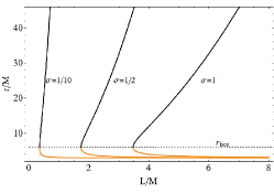
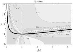
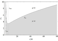
Figure 1: (Color online) Left panel: $r_{\mbox{\tiny{L}}}^{+}/M$ (black line) and $r_{\mbox{\tiny{L}}}^{-}/M$ (orange line) as a function of $L/M$ for different $\sigma$. The dashed line marks $r_{\mbox{\tiny{L}}}^{+}=r_{\mbox{\tiny{L}}}^{-}=r_{lsco}$. This condition is fulfilled when $\mathcal{L}=2\sqrt{3}$. Center panel: $G_{r}=\mbox{constant}$ as a function of $\ell$ and $r/M$. The singularity at $\ell=\ell_{r}$ is marked with a thick black line. Dashed line marks $r=r_{lco}$. Right panel: $\mathbf{\mathcal{L}_{\mbox{\tiny{K}}}=L_{\mbox{\tiny{K}}}/(M\sigma)}$ as a function of $r/M$. $p^{\prime}>0$ (and $p^{\prime}<0$) in the white (gray) region. $G_{r}=0$ when $L=L_{\mbox{\tiny{K}}}$ (solid line). Dashed line marks $r=r_{{lsco}}$, dotted line $r=r_{{lco}}$.

We are now interested in finding explicitly the critical points for the pressure, i.e. to find the solutions to Eq. 12. For a test particle within the effective potential $V_{sc}$, the angular momentum $L$ is a constant of motion. The particle motion is then described by $V^{\prime}_{sc}=0$ (the prime $(^{\prime})$ stays for the derivative with respect to $r$), which is equivalent to Eq. 12. Therefore, the circular orbit radii for a test particle in Schwarzschild spacetime:

$$r^{\pm}_{\mbox{\tiny{L}}}\equiv\frac{L^{2}}{2\sigma^{2}M^{2}}\left(M\pm\sqrt{L^{2}-12\sigma^{2}M^{2}}\right)=\frac{\mathcal{L}^{2}}{2}\left(M\pm\sigma M\sqrt{\mathcal{L}^{2}-12}\right)$$ (15)

are solutions to Eq. 12. $r_{\mbox{\tiny{L}}}^{+}$ corresponds to the test particle stable orbit, and $r_{\mbox{\tiny{L}}}^{-}$ to the unstable orbit. The isobar surfaces ($G_{r}=0$) are therefore located at $r=r_{\mbox{\tiny{L}}}^{\pm}$. Figure 1left panel describes the behavior of $r_{\mbox{\tiny{L}}}^{\pm}$ as a function of $L$ and $\sigma$. We underline that the matter distribution around the accretor is not spherically symmetric, and hence it is not independent on $\sigma$. A complete characterization of the equipotential surfaces as a function of $\sigma$ can be found in Appendix (A).

3.2 Angular momentum $L$ vs. fluid angular momentum $l$

It is also possible to describe the motion of the fluid orbiting in the Schwarzschild background in terms of its angular momentum $l$, defined as:

$$l\equiv\frac{g_{\varphi\varphi}}{g_{tt}}\frac{\Phi}{\Sigma}=\frac{L}{V_{sc}}\,,$$ (16)

In fact, equipotential surfaces define the marginally stable configurations with respect to the axisymmetric perturbation (, Seguin1975), characterized by $l$ constant. These configurations have been detailed studied in (Kozłowski et al.1978). From Eq. 16 and the definition of the effective potential in Eq. 7 the following relation holds:

$$L^{2}=\frac{r^{2}\sigma^{2}}{e^{-\nu}r^{2}\sigma^{2}l^{-2}-1}\quad(l\neq 0)\,.$$ (17)

The boundary case $l=0$ corresponds to $L=0$.

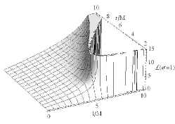
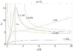
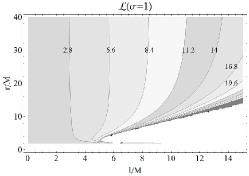
Figure 2: Left panel: $\mathcal{L}$ on the equatorial plane $\sigma=1$ as a function of $l/M\in[0,10]$ and $r/M\in]2,10]$. Central panel: $\mathcal{L}(\sigma=1)$ as a function of $r/M$, for different $l$. Asymptotically ($r\rightarrow\infty$), it is $L\rightarrow l$. The dotted-dashed curve marks $l=l_{r}$ as a function of $r/M$: the angular momentum $L$ is defined for $l<l_{r}$. $r_{\mbox{\tiny{lco}}}$ is a minimum of $l_{r}$. Right panel: $\mathcal{L}(\sigma=1)=\rm{constant}$ as a function of $r/M$ and $l/M$.

We detail the angular momentum $L$ on the equatorial plane $\sigma=1$ as a function of $l\neq 0$ and $r$ in Figs. 2. The two definitions of angular momentum coincide in the asymptotic limit of flat spacetime ($r\rightarrow\infty$). It is manifest from Fig. 2, central panel that it is $L=l=$constant for sufficiently large distances from the accretor. $L$ is not defined everywhere in the plane $(r,l)$: from Eq. 17, we notice that $L$ exists for $0\leq l<l_{r}$, where:

$$l_{r}\equiv\sqrt{\frac{\sigma^{2}r^{3}}{(r-2M)}}\,,$$ (18)

is defined for $r>2M$. In the boundary case $r=2M$, $L=0$. For fixed $\sigma$, $l_{r}$ is increasing for $r>r_{lco}$, is minimum for $r=r_{lco}$, and is deceasing for $2M<r<r_{lco}$. It is also progressively larger when approaching the equatorial plane $\sigma=1$, where it is maximum.

We now face the problem of finding a relation to link $(r,\sigma)$ and $l$ to the condition of the existence of $L$, and therefore of the velocity of the fluid $\Phi$. For this purpose we re-define the radii in Eq. 15:

$$r^{+}_{l}/M \equiv \frac{2\sqrt{\ell^{2}}\cos\left[\frac{1}{3}\arccos\left(-\frac{3\sqrt{3}}{\sqrt{\ell^{2}}}\right)\right]}{\sqrt{3}},\quad r^{-}_{l}/M\equiv-\frac{2{\sqrt{\ell^{2}}}\sin\left[\frac{\pi}{6}-\frac{1}{3}\arccos\left(-\frac{3\sqrt{3}}{{\sqrt{\ell^{2}}}}\right)\right]}{\sqrt{3}},$$ (19)

introducing the dimensionless quantity $\ell\equiv l/(\sigma M)>0$ ($\ell_{r}\equiv l_{r}/(\sigma M)$). With this definition, $r^{+}_{l}=r^{-}_{l}=r_{lco}$ for $\ell=3\sqrt{3}$. $r^{-}_{l}$ approaches the horizon $r=2M$ as the angular momentum $\ell$ increases (see Fig. 3 upper right panel). The angular momentum $L$ and the velocity $\Phi$ are not defined inside the region $[r^{-}_{l},r^{+}_{l}]$ (see Figs. 3 bottom panel and upper left panel). The region $[r^{-}_{l},r^{+}_{l}]$ increases with $\ell$. It varies also for different $\sigma$: its behavior as a function of $\sigma$ is detailed in Appendix A.

Now, we investigate the critical points of the angular momentum $L$ as function of $r$, solutions of $L^{\prime}=0$. For $r>r_{lco}$, $L$ is a constant with respect to the orbital radius when $l=l_{\mbox{\tiny{K}}}$, where

$$l_{\mbox{\tiny{K}}}/M=\sqrt{\frac{\sigma^{2}r^{3}}{M(r-2M)^{2}}}$$ (20)

is the Keplerian angular momentum of the fluid. The critical points of $L$ are, thus:

$$r_{-}/M \equiv \frac{1}{3}\left(\ell^{2}-2\sqrt{\ell^{2}\left(\ell^{2}-12\right)}\cos\left[\frac{1}{3}\left(\pi+\arccos\left[\frac{\ell^{2}\left(54-18\ell^{2}+\ell^{4}\right)}{\left(\ell^{2}\left(\ell^{2}-12\right)\right)^{3/2}}\right]\right)\right]\right)\,,$$ (21)

$$r_{+}/M \equiv \frac{1}{3}\left(\ell^{2}+2\sqrt{\ell^{2}\left(\ell^{2}-12\right)}\cos\left[\frac{1}{3}\arccos\left(\frac{\ell^{2}\left(54-18\ell^{2}+\ell^{4}\right)}{\left[\ell^{2}\left(\ell^{2}-12\right)\right]^{3/2}}\right)\right]\right)\,,$$ (22)

where $r_{-}\leq r_{+}$, and $r_{-}=r_{+}=r_{lsco}$ when $\ell=3\sqrt{{3}/{2}}$.

The angular momentum $L$ is a decreasing function of $r/M$ in all $r>r_{{lco}}$ with $\ell_{\mbox{\tiny{K}}}<\ell<\ell_{r}$, it increases with $r$ in $2M<r\leq r_{lco}$ with $0<\ell<\ell_{r}$ and in $r>r_{lco}$ for $0<\ell<\ell_{\mbox{\tiny{K}}}$ (see Figs. 3).

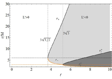
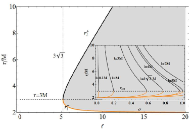
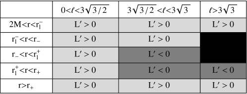
Figure 3: (Color online) Upper left panel $r_{\pm}$ and $r^{\pm}_{l}$ as a function of $\ell$. $r_{+}=r_{-}=r_{lsco}=6M$ (dashed line) when $\ell=3\sqrt{3/2}$ (dotted-dashed line). $r^{+}_{l}=r^{-}_{l}=r_{lco}=3M$ (dashed orange line) when $\ell=3\sqrt{3}$ (dotted line). White region corresponds to $L^{\prime}>0$, light gray region to $L^{\prime}<0$. In the gray region the function $L$ is not defined. Upper right panel $r_{l}^{+}$ (black curve) and $r_{l}^{-}$ (orange curve) as a function of $\ell=l/(\sigma M)$. $r_{l}^{+}=r_{l}^{-}=3M$ (dashed line) when $\ell=3\sqrt{3}$ (dotted line). $L$ is not defined in the gray region. Inset panel $r_{l}^{+}$ (black curve) and $r_{l}^{-}$ (orange curve) as a function of $\sigma$ for different values of $l$. Dashed line marks $r=r_{lco}$, where $r_{l}^{+}=r_{l}^{-}$. Lower panel table summarizing the intervals where $L^{\prime}>0$ (light-gray) or $L^{\prime}<0$ (gray). Black boxes correspond to the interval $[r_{-},r_{+}]$, where the function $L$ is not defined.

3.3 Radial pressure gradient $G_{r}(l)$ vs fluid angular momentum $l$

The radial gradient $G_{r}$, as a function of $\ell=l/(\sigma M)$, can be written as:

$${G_{r}=-\frac{Mr^{3}-\ell^{2}M^{2}(r-2M)^{2}}{r(r-2M)\left[r^{3}-\ell^{2}M^{2}(r-2M)\right]}\,,}$$ (23)

for $\sigma\neq 0$ (see Figs. 1). It is not defined in $\ell=\ell_{r}=\sqrt{r^{3}/M^{2}(r-2M)}$ and in $r=r^{\pm}_{l}$.

We studied the sign of $G_{r}$ as a function of $L$ in Sect. 3.1: here we face the problem for $G_{r}$ as a function of $\ell$, the fluid constant of motion. In Appendix A, we will discuss the $G_{r}$ sign in terms of $(l,\sigma,r)$ explicitly. According with the results found in Sect. 3.2, $G_{r}=0$ (isobar surfaces) for the radii $r_{\pm}$ with Keplerian angular momentum $\ell_{\mbox{\tiny{K}}}$. Thus, ${G_{r}<0}$ in:

$$2M<r\leq r_{lco}\quad\mbox{for}\quad 0\leq\ell<\ell_{r}\quad\mbox{and}\quad\ell>\ell_{\mbox{\tiny{K}}}\,,$$

$$r>r_{lco}\quad\mbox{for}\quad 0\leq\ell<\ell_{\mbox{\tiny{K}}}\quad\mbox{and}\quad\ell>\ell_{r}\,.$$

In terms of the radii $r_{\pm}$ and $r^{\pm}_{l}$, ${G_{r}>0}$ in:

$$0\leq\ell<3\sqrt{{3}/{2}} r>2M\,,$$ in

$$\ell=3\sqrt{{3}/{2}} r>2M,\quad r\neq r_{lsco}\,,$$ in

$$3\sqrt{{3}/{2}}<\ell\leq 3\sqrt{3} 2M<r<r_{-},\quad r>r_{+}\,,$$ in

$$\ell>3\sqrt{3} 2<r<r_{l}^{-},\quad r_{-}<r<r_{l}^{+},\quad r>r_{+}\,.$$ in

These intervals are portrayed in Figs. 4 upper panels.

In Sect. 3.2 we verified that $L^{\prime}(l_{\mbox{\tiny{K}}})=0$, where $L(l_{\mbox{\tiny{K}}})=L_{\mbox{\tiny{{K}}}}$ for $r>r_{lco}$. Here we showed that $l_{\mbox{\tiny{K}}}$ satisfies the condition $G_{r}(l_{\mbox{\tiny{K}}})=0$ and therefore we can claim that $l_{\mbox{\tiny{K}}}$ is also a critical point for the pressure $p$. This is illustrated in Figs. 4.

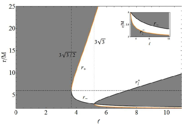
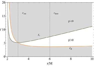
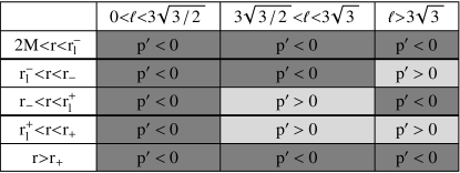
Figure 4: (Color online) Upper left panel: $r_{\pm}$ and $r_{l}^{\pm}$ as a function of $\ell$. White regions correspond to $p^{\prime}>0$ and gray regions to $p^{\prime}<0$. Radii $r_{l}^{\pm}$ are defined for $\ell>3\sqrt{3}$: the gradient $G_{r}$ is not defined in $r^{\pm}_{l}$. For $3\sqrt{3/2}<\ell<3\sqrt{3}$ the radius $r_{-}$ is a minimum of the pressure, and $r_{+}$ is a maximum. For $\ell>3\sqrt{3}$ the radius $r_{-}$ and $r_{+}$ are both maximum of the pressure. $r_{\pm}$, and $r^{\pm}_{l}$ are plotted as a function of $\ell$, $r_{+}=r_{-}=r_{lsco}$ (dashed line) when $\ell=3\sqrt{3/2}$ (dotted-dashed line). $r^{+}_{l}=r^{-}_{l}=r_{lco}$ when $\ell=3\sqrt{3}$ (dotted line). Inset: zoom of the region $r/M\in[2,3]$. Right panel: $\ell_{r}$ (black line) and $\ell_{\mbox{\tiny{K}}}$ (orange line) as a function of $r/M$. $\ell_{r}=\ell_{\mbox{\tiny{K}}}=3\sqrt{3}$ in $r=r_{lco}$ (dashed line), where ${G_{r}=-(1/3)M^{-1}}$. The function is not defined in $\ell=\ell_{r}$, while $G_{r}=0$ in $\ell=\ell_{\mbox{\tiny{K}}}$. In the gray regions $p^{\prime}<0$, in the white regions $p^{\prime}>0$ . The angular momentum $\ell_{\mbox{\tiny{K}}}$ has a minimum in $r_{lsco}$ (dashed line). Lower panel: table summarizing the regions of increasing ($p^{\prime}>0$–light-gray shaded regions) and decreasing ($p^{\prime}<0$–gray shaded regions) pressure $p$.

4 The polar angular pressure gradient $G_{\vartheta}$

We now concentrate our attention on the polar angular pressure gradient $G_{\vartheta}$. From Eq. 10:

$${G_{\vartheta}\equiv\frac{\nabla_{\vartheta}p}{\rho+p}\,}$$ (24)

On the equatorial plane $\sigma=1$, it is $\nabla_{\vartheta}p=0$: the angular gradient of pressure on the equatorial plane is always zero. $\partial_{\vartheta}p=0$ also for $L=0$. This implies that the case $L=0$ leads to a zero polar gradient of $p$, while ${G_{r}(L=0)=-{M}/((r-2M)r)<0}$, i.e. the pressure decreases as $1/r^{2}$ as approaching the horizon $r=2M$.

For $L=L_{\mbox{\tiny{K}}}$, $\partial_{r}p=0$ and therefore $p$ is a function of $\vartheta$ only. In general, for $\sigma\neq 1$ it is $\nabla_{\vartheta}p(L=L_{\mbox{\tiny{K}}})\neq 0$. In fact it results:

$$G_{\vartheta}(L=L_{\mbox{\tiny{K}}})\equiv\frac{\nabla_{\vartheta}p(L_{\mbox{\tiny{K}}})}{\rho+p}=\frac{M\sqrt{1-\sigma^{2}}}{\sigma(r-3M)},$$ (25)

(see Figs. 5). The quantity in Eq. 25 is not defined in $r=r_{{lco}}$ and, as for $L_{\mbox{\tiny{K}}}$, in the region $r\in(2M,r_{lco}]$. This means that there is a fluid configuration with pressure constant along the orbital radius and a pressure variable from plane to plane extended at radial distance $r>r_{lco}$. $G_{\vartheta}(L=L_{\mbox{\tiny{K}}})$ admits critical points for $\sigma=1$.

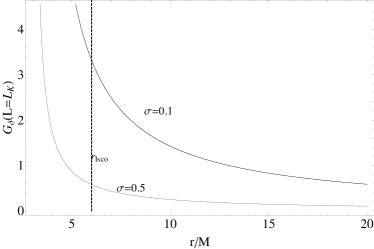
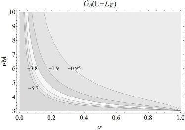
Figure 5: left panel: $G_{\vartheta}(L=L_{\mbox{\tiny{K}}})$ as a function of $r/M\in]3,20]$ for different values of $\sigma$. The black dashed line marks $r=r_{lsco}$. No solutions of $\partial_{\vartheta}p=0$, and no test particle circular orbits exist for $r/M\in(2,3]$. Right panel: Curves $G_{\vartheta}(L=L_{\mbox{\tiny{K}}})=$constant as a function of $r/M$ and $\sigma$.

4.1 Pressure gradient ratio $\Pi_{r\vartheta}$ vs angular momentum $L$

We define the pressure gradient ratio $\Pi_{r\vartheta}=\Pi_{r\vartheta}(L,r,\sigma)$ as $\Pi_{r\vartheta}\equiv{\nabla_{r}p}/{\nabla_{\vartheta}p}$. It is clearly $\Pi_{r\vartheta}=0$ for $L=L_{\mbox{\tiny{K}}}$ and it is not defined in $\sigma=1$. We rewrite this function as:

$$\Pi^{L}_{r\vartheta}\equiv\left|\cot\vartheta\Pi_{r\vartheta}M\right|=\frac{\left|r^{2}-M\mathcal{L}^{2}(r-3M)\right|}{\mathcal{L}^{2}r(r-2M)},$$ (26)

This ratio is equal to one for:

$$\mathcal{L}_{\Pi}\equiv\sqrt{\frac{r^{2}}{r(r-M)-3M^{2}}}\,,\quad r_{\Pi}^{L}/M\equiv\frac{1}{2}\left[\frac{\mathcal{L}^{2}}{\mathcal{L}^{2}-1}+\sqrt{\frac{\mathcal{L}^{2}\left(13\mathcal{L}^{2}-12\right)}{\left(\mathcal{L}^{2}-1\right)^{2}}}\right]\,.$$ (27)

The ranges where $\Pi^{L}_{r\vartheta}$ is larger, lower or equal to one are summarized in Fig. 6, left panel.

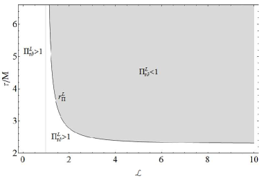
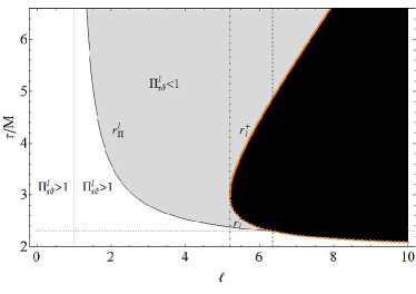
Figure 6: (Color online) Left panel: $r_{\Pi}^{L}$ as a function of $\mathcal{L}$. Black line marks $\mathcal{L}=1$. In the light gray region $\Pi^{L}_{r\vartheta}<1$, in the white region $\Pi^{L}_{r\vartheta}>1$. Right panel: $r_{\Pi}^{l}$, $r^{\pm}_{l}$ as a function of $\ell$. Black line marks the value $\ell=1$, dashed line $\ell\simeq 6.35$, dotted-dashed line $\ell=3\sqrt{3}$, dotted line $r=\frac{1}{2}\left(1+\sqrt{13}\right)M$. In the black region $r^{-}_{l}<r<r^{+}_{l}$ the function $\Pi^{l}_{r\vartheta}$ is not defined. In the gray region $\Pi^{l}_{r\vartheta}<1$, in the white region $\Pi^{l}_{r\vartheta}>1$. In $r=r_{\Pi}^{l}$ (black line) it is $\Pi^{l}_{r\vartheta}=1$.

4.2 Analysis of the pressure gradient ratio $\Pi_{r\vartheta}$ vs angular momentum $l$

We consider now the ratio $\Pi_{r\vartheta}$ as function of $l$. We then define the function $\Pi^{l}_{r\vartheta}=\Pi^{l}_{r\vartheta}(r,\ell)$:

$$\Pi^{l}_{r\vartheta}\equiv\left|\cot\vartheta M\Pi_{r\vartheta}\right|=\frac{\left|r^{3}-\ell^{2}M(r-2M)^{2}\right|}{\ell^{2}r(r-2M)^{2}},$$ (28)

in the range of existence of $L(l)$. Then we exclude the range $r^{-}_{l}\leq r\leq r^{+}_{l}$. The solution of $\Pi^{l}_{r\vartheta}=1$ are $r=r_{\Pi}^{l}>M(1+\sqrt{13})/2$ and $\ell=\ell_{\Pi}\in(1,\ell_{(\Pi-)})$, where $\ell_{(\Pi-)}=\sqrt{\left(41+11\sqrt{13}\right)/2}=6.35063$ satisfies the condition $r_{\Pi}^{l}(\ell_{(\Pi-)})=r_{l}^{-}(\ell_{(\Pi-)})\approx 2.30278\,M$ (see Fig. 6, right panel), with:

$$\ell_{\Pi}\equiv\sqrt{\frac{r^{3}}{(r+M)(r-2M)^{2}}}\,,$$ (29)

and

$$r_{\Pi}^{l}/M\equiv\frac{\ell^{2}}{\ell^{2}-1}+2\ell^{2}\sqrt{\frac{1}{\left(\ell^{2}-1\right)^{2}}}\cos\left(\frac{1}{3}\arccos\left[\frac{1}{\ell^{4}}\sqrt{\frac{1}{\left(\ell^{2}-1\right)^{2}}}\left(1-\ell^{2}\right)\left(\ell^{4}-4\ell^{2}-2\right)\right]\right)\,.$$ (30)

The ranges where $\Pi^{l}_{r\vartheta}$ is larger, lower or equal to one are summarized in Fig. 6, right panel.

5 The Boyer potential

The disk fluid configuration in the Polish doughnut model has been widely studied by many authors (see for example Frank et al.2002, Abramowicz& Fragile2011). In particular, an analytic theory of equilibrium configurations of rotating perfect fluid bodies was initially developed by (Boyer1965). The “Boyer’s condition” states that the boundary of any stationary, barotropic, perfect fluid body has to be an equipotential surface $W(l,\vartheta)=\mbox{constant}$. For a barotropic fluid the surfaces of constant pressure are given by the equipotential surfaces of the potential defined by the relation:

$$\int_{0}^{p_{in}}\frac{dp}{\rho+p}=-(W-W_{in}),$$ (31)

where the subscript “in” refers to the inner edge of the disc. It is important to notice here that, in the newtonian limit, the quantity $W$ is equal to the total potential, i.e. to the sum of the gravitational and of the centrifugal effects.

As mentioned in Sect. 3.2, all the main features of the equipotential surfaces for a generic rotation law $\Omega=\Omega(l)$ are described by the equipotential surface of the simplest configuration with uniform distribution of the angular momentum density $l$, which are very important being marginally stable (, Seguin1975). At the same time, the equipotential surfaces of the marginally stable configurations orbiting in a Schwarzschild spacetime are defined by the constant $l$. It is therefore important to study the potential $W=W(l,\sigma)$ and to compare it with $W=W(L,\sigma)$.

We can classify the equipotential surfaces in three classes: closed, open, and with a cusp (self-crossing surfaces, which can be either closed or open). The closed equipotential surfaces determine stationary equilibrium configurations: the fluid can fill any closed surface. The open equipotential surfaces are important to model some dynamical situations, for example the formation of jets (see e.g. , Kucakova et al.2011, Stuchlík et al.2009, Lei et al.2009, Abramowicz et al.1998, Stuchlík & Slaný2006, Abramowicz2009, Stuchlík & Kovář2008, Rezzolla et al.2003, Stuchlíkl2000, Slaný & Stuchlík2005, Stuchlík et al.2000).

The critical, self-crossing and closed equipotential surfaces are relevant in the theory of thick accretion disks, since the accretion onto the black hole can occur through the cusp of the equipotential surface. According to Paczyński (, Abramowicz et al.1978, Kozłowski et al.1978, Jaroszynski et al.1980, Abramowicz1981), the accretion onto the source (black hole) is driven through the vicinity of the cusp due to a little overcoming of the critical equipotential surface $W_{cusp}$ by the surface of the disk. The accretion is thus driven by a violation of the hydrostatic equilibrium, clearly ruling out the viscosity as a basis for accretion (, Kozłowski et al.1978). In the Paczyński mechanism the disk surface exceeds the critical equipotential surface $W_{cusp}$ giving rise to a mechanical non-equilibrium process that allows the matter inflow into the black hole. In this accretion model the cusp of this equipotential surface corresponds to the inner edge of the disk.

We calculate now the Boyer potential for our system integrating Eq. 11:

$$\int^{p_{out}}_{p_{in}}\frac{dp}{\rho+p}=-\int_{r_{in}}^{r_{out}}\frac{e^{-\nu}}{2}\left(\frac{\partial V_{sc}^{2}}{\partial r}\right)_{L}.$$ (32)

The integration range $[r_{in},r_{out}]\subset[2M,\infty]$ is the range of existence for $V_{sc}(r,l)$, $(r-2M)\left[r^{3}-\ell^{2}M^{2}(r-2M)\right]>0$. This condition implies that we are excluding the range $[r_{l}^{-},r_{l}^{+}]$. The general integral is:

$$\int\frac{dp}{\rho+p}=-W,$$ (33)

where

$$W=\ln\left[\sqrt{\frac{(r-2M)r^{2}}{r^{3}-\ell^{2}M^{2}(r-2M)}}\right]=\ln V_{{sc}}.$$ (34)

In particular it results:

$$\lim_{r\rightarrow\infty}W=0,\quad\lim_{r\rightarrow 2M}W=+\infty$$ (35)

(see also , Stuchlík et al.2000, Stuchlík & Kovář2008, Abramowicz2005, Stuchlík & Slaný2006, Slaný & Stuchlík2005, Abramowicz et al.1980, Rezzolla et al.2003). Clearly it is $W=0$ where $V_{sc}=1$, and $W\gtrless 0$ where $V_{sc}\gtrless 1$. Its maxima and minima are the same than the Schwarzschild effective potential, $V_{sc}=V_{sc}(l,r)$. In particular, we are interested to study the equipotential surfaces, defined by the condition $W=\rm{constant}$, that coincide with the surfaces $V_{sc}=\rm{K}>0$, being $\rm{K}\equiv e^{c}$ the energy of a test particle circularly orbiting around the source. In fact the surfaces of constant Boyer potential determine the shape of the torus (disc). We study these surfaces as a function of $L=\mbox{constant}$ and $l=\mbox{constant}$, respectively.

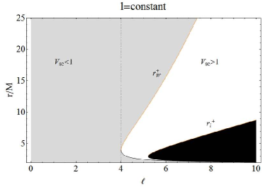
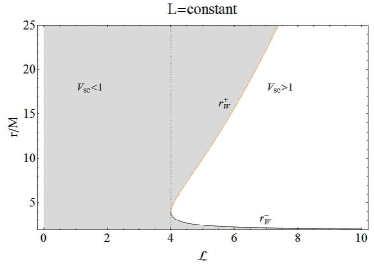
Figure 7: (Color online) Left panel: $r_{W}^{+}$ (orange curve) and $r_{W}^{-}$ (black curve) as a function of $\ell$. The black region $r^{-}_{l}<r<r_{l}^{+}$) is forbidden. $V_{sc}>1$ in the white region, $V_{sc}<1$ in the gray region. Dotted line marks $\ell=4$. Right panel: $\tilde{r}_{W}^{+}$, (orange curve) and $\tilde{r}_{W}^{-}$ (black curve) as function of $\mathcal{L}$. $V_{sc}>1$ in the white region, $V_{sc}<1$ in the gray region. Dotted line marks $\mathcal{L}=4$.

5.1 Analysis of the Boyer potential vs the angular momentum $L$

We consider the Boyer potential $W(L,r)$ in Eq. 34 as function of the angular momentum $L$. The condition $W=0$ is satisfied in:

$$\tilde{r}_{W}^{\pm} \equiv \frac{M}{4}\left(\mathcal{L}^{2}\pm\sqrt{\mathcal{L}^{2}(\mathcal{L}^{2}-16)}\right)$$ (36)

(see Fig. 7, right panel).

We notice that two relevant cases occur when the angular momentum is ${\mathcal{L}^{2}=\mathcal{L}_{k}^{2}}$, where ${{\mathcal{L}}_{k}^{2}\equiv\frac{r^{2}\left[2M+\left(\rm{K}^{2}-1\right)r\right]}{M^{2}(r-2M)}}$: (I) when $0<\rm{K}<1$, $W<0$, in $2M<r\leq\tilde{r}_{\rm{K}}$, where $\tilde{r}_{\rm{K}}\equiv\frac{2M}{1-\rm{K}^{2}}$; (II) when $\rm{K}\geq 1$, $W\geq 0$ in $r>2M$.

The solutions of the equation $W=\ln(\rm{K})$ can be describer in terms of the energies:

$$\tilde{\rm{K}}_{\pm}\equiv\sqrt{\frac{1}{54}\left(36\pm\sqrt{\frac{(\mathcal{L}^{2}-12)^{3}}{\mathcal{L}^{2}}}+\mathcal{L}^{2}\right)},\quad\tilde{\rm{K}}_{\alpha}\equiv\frac{1}{\sqrt{3}}\sqrt{\frac{3\mathcal{L}^{2}-4}{\mathcal{L}^{2}}},$$ (37)

of the radii:

$$\tilde{r}_{k_{1}}/M \equiv -\frac{2+2\varpi\sin\left[\frac{1}{6}\left(\pi+2\arccos\psi\right)\right]}{3\left(\rm{K}^{2}-1\right)},$$ (38)

$$\tilde{r}_{k_{2}}/M \equiv -\frac{2+2\varpi\cos\left[\frac{1}{3}\left(\pi+\arccos\psi\right)\right]}{3\left(\rm{K}^{2}-1\right)},$$ (39)

$$\tilde{r}_{k_{3}}/M \equiv \frac{-2+2\varpi\cos\left(\frac{1}{3}\arccos\psi\right)}{3\left(\rm{K}^{2}-1\right)},$$ (40)

(see Figs. 8), where:

$$\psi\equiv-\frac{8+9\left(3\rm{K}^{4}-5\rm{K}^{2}+2\right)\mathcal{L}^{2}}{\varpi^{3}},\quad\varpi\equiv\left(\rm{K}^{2}-1\right)\sqrt{\frac{4+3\left(\rm{K}^{2}-1\right)\mathcal{L}^{2}}{\left(\rm{K}^{2}-1\right)^{2}}},$$ (41)

and of the angular momenta:

$$\mathcal{L}^{2}_{\alpha}\equiv\frac{4}{3\left(\rm{K}^{2}-1\right)},\quad{(\mathcal{L}_{K}^{\pm})}^{2}\equiv{\frac{1}{2}\left[\frac{27\rm{\rm{K}}^{4}-36\rm{K}^{2}+8}{\rm{K}^{2}-1}\pm\sqrt{\frac{\rm{K}^{2}\left(9\rm{K}^{2}-8\right)^{3}}{\left(\rm{K}^{2}-1\right)^{2}}}\right]},$$ (42)

These solutions are summarized in Figs. 9.

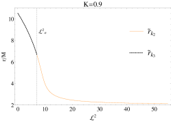
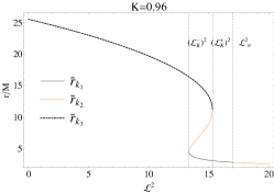
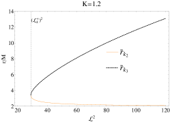
Figure 8: (Color online) $\tilde{r}_{k_{1}}$, $\tilde{r}_{k_{2}}$, $\tilde{r}_{k_{3}}$ as a function of $\mathcal{L}^{2}$ for different values of $\rm{K}$ in the ranges: $[0,2\sqrt{2}/3]$ (left panel), $[2\sqrt{2}/3,1]$ (central panel), $\rm{K}>1$ (right panel). Dotted lines are the momentum $\mathcal{L}^{2}_{\alpha}$ and $(\mathcal{L}_{K}^{\pm})^{2}$.

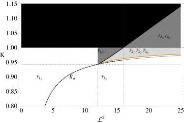
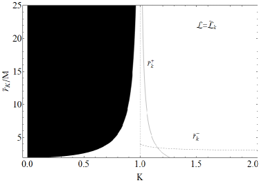
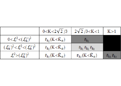
Figure 9: (Color online) Upper left panel: $\tilde{\rm{K}}^{+}$ (black curve), $\tilde{\rm{K}}^{-}$ (orange curve) and $\tilde{\rm{K}}_{\alpha}$ (dashed thick curve) as a function of $\mathcal{L}^{2}$. The regions of existence for the radii $\tilde{r}_{k_{1}},\tilde{r}_{k_{2}},\tilde{r}_{k_{3}}$, solution of $W=\ln(\rm{K})$ are marked in white, gray, light-gray. Black regions are forbidden. Dotted-dashed line marks $\rm{K}=2\sqrt{2}/3$. Upper right panel: $\tilde{r}_{\rm{K}}$ as a function of $\rm{K}$. Gray curve is $\tilde{r}_{k}^{+}$, dashed curve $\tilde{r}_{k}^{-}$. In the white region $\mathcal{L}^{2}={\mathcal{L}^{2}}_{k}$ solution of $W=\ln(\rm{K})$. No solution exists in the black region. Lower panel: table summarizing the regions of existence of the radii $\tilde{r}_{k_{1}},\tilde{r}_{k_{2}},\tilde{r}_{k_{3}}$. Black boxes are forbidden.

The critical points of the angular momentum $\mathcal{L}^{2}_{k}$ are:

$$\tilde{r}_{k}^{\pm}/M=\frac{1}{2}\left[\sqrt{\frac{\rm{K}^{2}\left(9\rm{K}^{2}-8\right)}{\left(\rm{K}^{2}-1\right)^{2}}}\pm\frac{3\rm{K}^{2}-4}{\rm{K}^{2}-1}\right]\,.$$ (43)

When $2\sqrt{2}/{3}<\rm{K}<1$ there are two critical points $\tilde{r}_{k}^{\pm}$, while when $\rm{K}>1$ there is only $r=\tilde{r}_{k}^{+}$ (see Fig. 9, upper right panel). For $\rm{K}=1$ it is $\tilde{r}_{k}^{\pm}=r_{mbo}$, where $r_{mbo}=4M$ is the marginally bounded orbit for a test particle in the Schwarzschild spacetime, and in $\rm{K}=2\sqrt{2}/3$ it is $\tilde{r}_{k}^{\pm}=r_{lsco}$.

Closed surfaces: the conditions for the existence of closed surfaces can be obtained by noting that, in cartesian coordinate $(x,y)$, the closed surfaces should satisfy the condition $V_{sc}(x=0)=\rm{K}$ with three solutions, say $y=\{y_{1},y_{2},y_{3}\}$. The closed surfaces then exist when ${2\sqrt{2}}/{3}<\rm{K}<1$ and $(\mathcal{L}_{\rm{K}}^{-})^{2}<\mathcal{L}^{2}<({\mathcal{L}_{\rm{K}}^{+}})^{2}$ (see Fig. 9, lower panel), with $(\mathcal{L}_{\rm{K}}^{-})^{2}\geq 16$. In cartesian coordinate $(x,y)$ the surfaces $V_{sc}=\rm{K}$ are:

$$x=\pm\sqrt{\frac{\left(2L^{2}+2y^{2}\right)^{2}}{\left(L^{2}+y^{2}-y^{2}\rm{K}^{2}\right)^{2}}-y^{2}}.$$ (44)

The maximum diameter $(x=0)$ of the closed Boyer surface lies between the points $y=y_{2}$ and $y=y_{3}$, where

$${y_{1}}/M \equiv \sqrt{\frac{1}{9}\left(\varsigma-6\theta\sin\left[\frac{1}{6}(\pi+2\arccos\varepsilon)\right]\right)},$$ (45)

$${y_{2}}/M \equiv \sqrt{\frac{1}{9}\left(\varsigma-6\theta\cos\left[\frac{1}{3}(\pi+\arccos\varepsilon)\right]\right)},$$ (46)

$${y_{3}}/M \equiv \sqrt{\frac{1}{9}\left[\varsigma+6\theta\cos\left(\frac{1}{3}\arccos\varepsilon\right)\right]},$$ (47)

being,

$$\theta \equiv \sqrt{\frac{16+8\left(3\rm{K}^{4}-4\rm{K}^{2}+1\right)(L/M)^{2}+\left(\rm{K}^{2}-1\right)^{2}(L/M)^{4}}{\left(\rm{K}^{2}-1\right)^{4}}},$$ (48)

$$\varepsilon \equiv \frac{64+48\left(3\rm{K}^{4}-4\rm{K}^{2}+1\right)(L/M)^{2}+6\left(\rm{K}^{2}-1\right)^{2}\left(9\rm{K}^{4}-6\rm{K}^{2}+2\right)(L/M)^{4}-\left(\rm{K}^{2}-1\right)^{3}(L/M)^{6}}{\left(\rm{K}^{2}-1\right)^{6}\theta^{3}},$$ (49)

$$\varsigma \equiv \frac{6\left[2+\left(\rm{K}^{2}-1\right)(L/M)^{2}\right]}{\left(\rm{K}^{2}-1\right)^{2}}$$ (50)

(see Fig. 10, left panel).

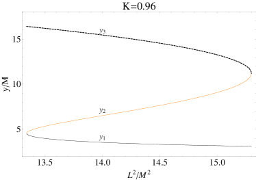
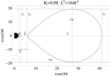
Figure 10: (Color online) Left panel: $y_{1}$ (black curve), $y_{2}$ (orange curve) and $y_{3}$ (dashed curve) as a function of $L^{2}$ for $\rm{K}=0.96$. Right panel: the closed Boyer surface at $K=0.98$ and $L^{2}=16M^{2}$. $\lambda\equiv y_{3}-y_{2}$ is the surface maximum diameter, $\delta\equiv y_{2}-2M$ is the distance from the source, $\hat{\delta}\equiv y_{2}-y_{1}$ is the distance from the inner surface, $\breve{\delta}\equiv y_{1}-2M$ is the distance of the inner surface from the horizon, $h\equiv 2x_{M}$ and $X_{h}\equiv y_{M}$.

Fig. 10, right panel portrays a closed Boyer surface. We can characterize this surface introducing the following parameters:

1. the surface maximum diameter: $\lambda\equiv y_{3}-y_{2},$

2. the distance from the source defined as: $\delta\equiv y_{2}-2M,$

3. the distance from the inner surface: $\hat{\delta}\equiv y_{2}-y_{1},$

4. the distance of the inner surface from the horizon: $\breve{\delta}\equiv y_{1}-2M,$

5. the surface maximum height defined as: $h\equiv 2x_{M},$

6. the quantity $X_{h}\equiv y_{M}.$

$(x_{M},y_{M})$ is the critical point of the surface in Eq. 44. In what follows we find the constraints for the set of parameters $\{\lambda,\delta,\hat{\delta},\breve{\delta},h,X_{h}\}$. The point $y_{3}$ varies in the range $2M<y_{3}<y_{s}$, and $L^{2}$ lies on the surface $L^{2}_{s}$, which is a solution of $V_{s}=K$ on the plane $x=0$ for $y>4M$ and $K\geq 1$, and for $4M<y<y_{s}$ for $K<1$:

$$y_{s}\equiv\frac{2M}{\left|\rm{K}^{2}-1\right|},\quad L^{2}_{s}=2M\sqrt{\frac{\rm{K}^{4}y^{6}}{(y^{2}-4M^{2})^{2}}}+y^{2}\left(\frac{\rm{K}^{2}y^{2}}{y^{2}-4M^{2}}-1\right)$$ (51)

(see Figs. 11). $\lambda$ increases with the energy $\rm{K}$, but decreases with the fluid angular momentum $L$. On the contrary, the distance from the source $\delta=y_{2}-2M$ increases with $L$ and decreases with $\rm{K}$ (see Figs. 11).

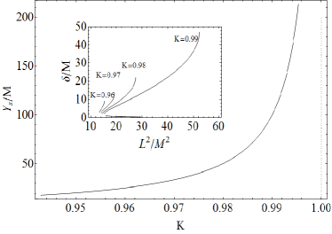
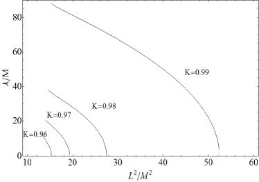
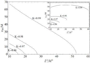
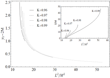
Figure 11: Upper left panel: $y_{s}$ as a function of the energy $2\sqrt{2}/3<K<1$. Inset: distance of the surface from the $r=2M$ $\delta\equiv y_{2}-2M$ as a function of $L^{2}$, for different values of $K$. It increases with $L^{2}$ and decreases with $\rm{K}$. Upper right panel: surface maximum diameter $\lambda\equiv y_{3}-y_{2}$ as a function of $L^{2}$ for different values of $K$. Lower left panel: maximum $x_{M}=x(y_{M})$ as a function of $L^{2}$ for different energies $K$. Inset: $y_{M}$ as a function of $L^{2}$, for different values of $K$. Lower right panel: distance $\breve{\delta}\equiv y_{1}-2M$ as a function of $L^{2}$, for different values of $K$. Inset: distance $\hat{\delta}=y_{2}-y_{1}$ as a function of $L^{2}$, for different values of $K$.

The maximum vertical distance of the closed surfaces is:

$$y_{M}/M=\sqrt{\frac{3(L/M)^{2}+4\sqrt{6}\left(\rm{K}^{2}-1\right)\sqrt{-\frac{\rm{K}^{2}(L/M)^{2}}{\left(\rm{K}^{2}-1\right)^{3}}}\cos\left[\frac{1}{3}\arccos\left[-\frac{3}{4}\sqrt{\frac{3}{2}}\left(\rm{K}^{2}-1\right)^{2}\sqrt{-\frac{\rm{K}^{2}(L/M)^{2}}{\left(\rm{K}^{2}-1\right)^{3}}}\right]\right]}{3\left(\rm{K}^{2}-1\right)}}.$$ (52)

As shown in Figs. 11, the maximum $x_{M}=x(y_{M})$, and consequently the height $h$, increases with $\rm{K}$ and decreases with $L^{2}$. On the contrary $y_{M}$ increases with $\rm{K}$ and with $L^{2}$, until it reaches a maximum and then decreases. The distance $\hat{\delta}=y_{2}-y_{1}$ increases with $L^{2}$ and decreases with $\rm{K}$. The distance $\breve{\delta}\equiv y_{1}-2M$ increases with the energy $\rm{K}$ and decreases with $L^{2}$.

Cusps: the cusps, i.e. the self-crossing surfaces $W=\rm{constant}$, correspond to the maxima of the effective potential as a function of $r$: open surfaces are maxima with energy $\rm{K}>1$, and closed surfaces are maxima with energy $\rm{K}<1$, as outlined in Fig. 12 upper. It is therefore important to consider the function $V^{\prime}$ in the regions of closed and open Boyer surfaces. From Sect. 3.1 we know that the solutions of the equations $V^{\prime}=0$ that correspond to maxima of the effective potential are located on the radius $r=r_{L}^{-}$, in particular there are closed surfaces with a cusps in $r_{L}^{-}>r_{mbo}$, and $12\leq\mathcal{L}^{2}<16$ , viceversa maxima located in $r_{L}^{-}>r_{mbo}$ with $\mathcal{L}^{2}\geq 16$ are open surfaces with a cusp (see Fig. 12 upper).

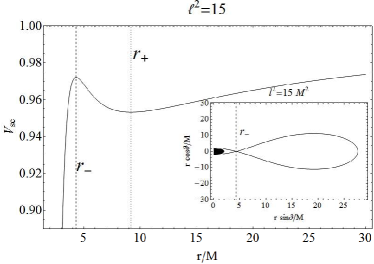
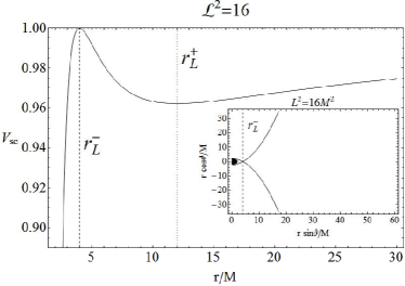
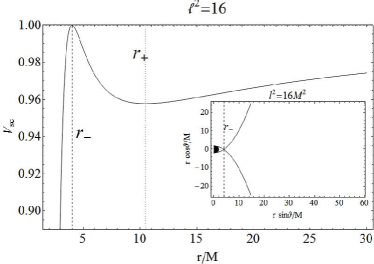
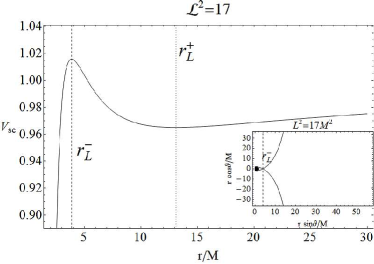
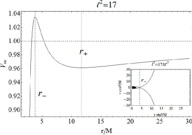
Figure 12: Left panels: Effective potential $V_{sc}(L,r)$ as a function of $r/M$, for selected values of $\mathcal{L}^{2}=L^{2}/M^{2}\sigma^{2}$. Dashed lines mark $r_{L}^{\pm}$. Inset: the self–crossing Boyes surfaces corresponding to the maxima of the effective potential as function of $r$: maximum with energy $\rm{K}>1$ are open surfaces and maximum with energy $\rm{K}<1$ are closed surfaces. Right panels: Plots of the effective potential $V_{sc}(l,r)$ as function of $r/M$, for selected values of ${\ell^{2}}=l^{2}/M^{2}\sigma^{2}$. Dashed lines are $r_{\pm}$. Correspondingly the self–crossing Boyer surfaces are plotted in the inner panel. They correspond to the maxima of the effective potential as function of $r$: maximum with energy $\rm{K}>1$ are open surfaces and maximum with energy $\rm{K}<1$ are closed surfaces.

Remark: integrating Eq. 32 with $V_{sc}$ as function of the constant of motion $L$, we obtain the following expression for the potential:

$${\widetilde{W}\equiv\frac{2\mathcal{L}^{4}M(r+3M)+\left(4+\mathcal{L}^{4}\right)r^{2}[\ln(r/M-2)-\ln(r/M)]}{8r^{2}}\,.}$$ (53)

The solutions of $\widetilde{W}=\rm{c}$ ensure the existence of closed, open and self–crossing surfaces.

5.2 Analysis of the Boyer potential vs the angular momentum $l$

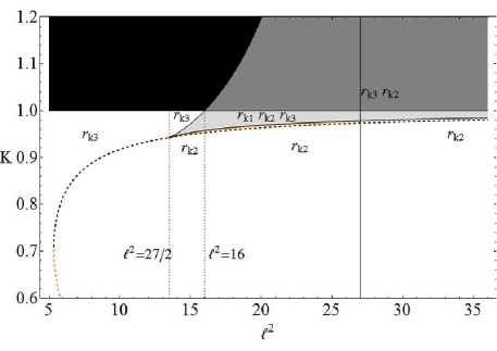
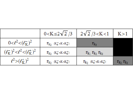
Figure 13: (Color online) Upper panel: ${\rm{K}}_{a}$ (black curve), ${\rm{K}}_{b}$ (orange curve), ${\rm{K}}_{\alpha}^{+}$ (dashed thick black curve) and ${\rm{K}}_{\alpha}^{-}$ (dashed thick orange curve) as a function of ${\ell^{2}}$. The colored regions mark the existence for the radii ${r}_{k_{1}},{r}_{k_{2}},{r}_{k_{3}}$. The black region is forbidden. Dotted lines are $\ell^{2}=16$ and $\ell^{2}=27/2$. Lower panel: table summarizing the regions of existence for the radii ${r}_{k_{1}},{r}_{k_{2}},{r}_{k_{3}}$. Black boxes are forbidden.

We face now the analysis of the Boyer potential in terms of the fluid angular momentum $l=\mbox{constant}$. Firstly, we note that the Boyer surface in Eq. 34 is not defined in the region $[r_{l}^{-},r_{l}^{+}]$. We detail the study of the sign of $V_{sc}(l,r)$ in Figs. 13 (see also Fig. 7, left panel). With respect to the case of $L=\rm{constant}$ (see Figs. 9 and Eqs. 37–42), here new definitions have been introduced for the energies:

$$\rm{K}_{a} \equiv \sqrt{\frac{\ell^{2}-36-2\beta_{1}\sin\left(\frac{1}{3}\arcsin\alpha_{1}\right)}{3\ell^{2}-81}},$$ (54)

$$\rm{K}_{b} \equiv \sqrt{\frac{\ell^{2}-36+2\beta_{1}\cos\left(\frac{1}{3}\arccos\alpha_{1}\right)}{3\ell^{2}-81}},$$ (55)

$$\rm{K}_{\alpha}^{\pm} \equiv \frac{1}{\sqrt{6}}\sqrt{3\pm\frac{\sqrt{3}\sqrt{\ell^{2}(3\ell^{2}-16)}}{\ell^{2}}},$$ (56)

with

$$\alpha_{1}\equiv\frac{\left(2^{3}3^{9}\right)-\left(108\sqrt{2}\right)^{2}\ell^{2}+\left(6\sqrt{51}\right)^{2}{\ell^{2}}^{2}-72{\ell^{2}}^{3}+{\ell^{2}}^{4}}{\ell^{2}\beta_{1}^{3}},\quad\beta_{1} \equiv (\ell^{2}-27)\sqrt{\frac{72+(\ell^{2}-24)^{2}}{(\ell^{2}-27)^{2}}},$$ (57)

angular momenta:

$${\ell}_{\alpha}^{2}\equiv-\frac{4}{3\rm{K}^{2}\left(\rm{K}^{2}-1\right)},\quad({\ell}^{\pm}_{k})^{2} \equiv \frac{1}{2}\left(\pm\sqrt{\frac{\left(9\rm{K}^{2}-8\right)^{3}}{\rm{K}^{2}\left(\rm{K}^{2}-1\right)^{2}}}+\frac{27\rm{K}^{4}-36\rm{K}^{2}+8}{\rm{K}^{2}\left(\rm{K}^{2}-1\right)}\right),$$ (58)

and radii:

$${r}_{k_{1}}/M \equiv -\frac{2\left[1+\varpi_{k}\cos\left(\frac{1}{3}\arccos\psi_{k}\right)\right]}{3\left(\rm{K}^{2}-1\right)},$$ (59)

$${r}_{k_{2}}/M \equiv \frac{2\left(-1+\varpi_{k}\cos\left[\frac{1}{3}\arccos\left(-\psi_{k}\right)\right]\right)}{3\left(\rm{K}^{2}-1\right)},$$ (60)

$${r}_{k_{3}}/M \equiv \frac{2\left[-1+\varpi_{k}\sin\left(\frac{1}{3}\arcsin\psi_{k}\right)\right]}{3\left(\rm{K}^{2}-1\right)},$$ (61)

where:

$$\psi_{k}\equiv\frac{8+9\rm{K}^{2}\left(3\rm{K}^{4}-5\rm{K}^{2}+2\right)\ell^{2}}{\varpi_{k}^{3}},\quad\varpi_{k}\equiv\left(\rm{K}^{2}-1\right)\sqrt{\frac{4+3\rm{K}^{2}\left(\rm{K}^{2}-1\right)\ell^{2}}{\left(\rm{K}^{2}-1\right)^{2}}}\,.$$ (62)

The surfaces $W(l,r)=\rm{constant}$ exist in all the spacetime with angular momentum $\ell^{2}=\ell^{2}_{k}$ and energy $\rm{K}=\rm{K}_{k}$, where:

$$\ell^{2}_{k} \equiv \frac{r^{2}\left[2M+\left(\rm{K}^{2}-1\right)r\right]}{\rm{K}^{2}M^{2}(r-2M)}<\frac{r^{3}}{M^{2}(r-2M)},\quad\rm{K}_{k}\equiv r\sqrt{\frac{r-2M}{r^{3}-\ell^{2}M^{2}(r-2M)}}.$$ (63)

In particular in the case $0<\rm{K}<1$ it is $2M<r\leq 2M/(1-\rm{K}^{2})$.

Closed surfaces: following the same procedure outlined in the previous Subsection for $V_{sc}(L,r)$, we find that closed surfaces of the Boyer potential in the cartesian coordinate $(x,y)$ are in the regions $2\sqrt{2}/3<\rm{K}<1$ and $({\ell}_{k}^{-})^{2}<{\ell^{2}}<({\ell}_{k}^{+})^{2}$, where ${\ell^{2}}_{k}^{-}>27/2$ (see Figs. 13). The surfaces are therefore:

$$x=\pm\sqrt{\left[\frac{2M\left(\rm{K}^{2}l^{2}+y^{2}\right)}{\rm{K}^{2}\left(l^{2}-y^{2}\right)+y^{2}}\right]^{2}-y^{2}}$$ (64)

(see Fig. 14, right panel).

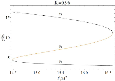
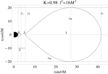
Figure 14: (Color online) Left panel: $y_{1}/M$ (black curve), $y_{2}/M$ (orange curve) and $y_{3}/M$ (dashed curve) as a function of $l^{2}/M^{2}$ for $\rm{K}=0.96$. Right panel: the closed Boyer surface at $K=0.98$ and $l^{2}=16M^{2}$. $\lambda\equiv y_{3}-y_{2}$ is the surface maximum diameter, $\delta\equiv y_{2}-2M$ is the distance from the source, $\hat{\delta}\equiv y_{2}-y_{1}$ is the distance from the inner surface, $\breve{\delta}\equiv y_{1}-2M$ is the distance of the inner surface from the horizon, $h\equiv 2x_{M}$ and $X_{h}\equiv y_{M}$.

The maximum diameter $(x=0)$, is defined by the points $y={y}_{2}$ and $y={y}_{3}$, where

$${y}_{1}/M \equiv \sqrt{\frac{1}{9}\left(\varsigma_{k}-6\theta_{k}\sin\left[\frac{1}{6}(\pi+2\arccos\varepsilon_{k})\right]\right)},$$ (65)

$${y}_{2}/M \equiv \sqrt{\frac{1}{9}\left(\varsigma_{k}-6\theta_{k}\cos\left[\frac{1}{3}(\pi+\arccos\varepsilon_{k})\right]\right)}$$ (66)

$${y}_{3}/M \equiv \sqrt{\frac{1}{9}\left(\varsigma_{k}+6\theta_{k}\cos\left[\frac{1}{3}\arccos\varepsilon_{k}\right]\right)},$$ (67)

(see also Eqs. 45–47), being

$$\theta_{k} \equiv \sqrt{\frac{16+8\rm{K}^{2}(l/M)^{2}+\rm{K}^{4}[(l/M)^{2}-32](l/M)^{2}-2\rm{K}^{6}[(l/M)^{2}-12](l/M)^{2}+\rm{K}^{8}(l/M)^{4}}{\left(\rm{K}^{2}-1\right)^{4}}},$$ (68)

$$\varepsilon_{k} \equiv \frac{64+K^{2}(l/M)^{2}\left(48+K^{2}\left[48\left(3K^{2}-4\right)+6\left(K^{2}-1\right)^{2}\left(9K^{4}-6K^{2}+2\right)(l/M)^{2}-K^{2}\left(K^{2}-1\right)^{3}(l/M)^{4}\right]\right)}{\left(\rm{K}^{2}-1\right)^{6}\theta_{k}^{3}},$$ (69)

$$\varsigma_{k} \equiv \frac{6\left[\rm{K}^{4}(l/M)^{2}-\rm{K}^{2}(l/M)^{2}+2\right]}{\left(\rm{K}^{2}-1\right)^{2}}\,,$$ (70)

(see Fig. 14, left panel).

The maximum height for the surface is:

$${y}_{M}/M \equiv \sqrt{\frac{3\rm{K}^{2}(l/M)^{2}+4\sqrt{6}\left(\rm{K}^{2}-1\right)\sqrt{-\frac{\rm{K}^{4}(l/M)^{2}}{\left(\rm{K}^{2}-1\right)^{3}}}\cos\left[\frac{1}{3}\arccos\left[-\frac{3}{4}\sqrt{\frac{3}{2}}\left(\rm{K}^{2}-1\right)^{2}\sqrt{-\frac{\rm{K}^{4}(l/M)^{2}}{\left(\rm{K}^{2}-1\right)^{3}}}\right]\right]}{3\left(\rm{K}^{2}-1\right)}}.$$ (71)

The surfaces for $l=\rm{constant}$ are larger then those for $L=\rm{constant}$. The two cases are compared in Figs. 15: the maximum diameter $\lambda(l)>\lambda(L)$; the distance from the source $\delta(l)>\delta(L)$; the distance of the inner surface from the horizon $\breve{\delta}(l)>\breve{\delta}(L)$; its maximum height $h(l)>h(L)$ and finally the quantity $x_{h}(l)>x_{h}(L)$; the distance from the inner surface $\hat{\delta}(l)<\hat{\delta}(L)$.

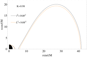
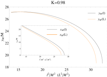
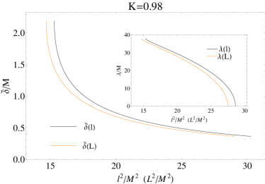
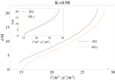
Figure 15: (Color online) Upper left panel: comparison of the closed Boyer surfaces with energy $\rm{K}=0.98$ and angular momentum $l^{2}=16M^{2}$ (black curves) and $L^{2}=16M^{2}$ (orange curve). It results $x(l^{2}=16M^{2})>x(L^{2}=16M^{2})$. Upper right panel: comparison of the surface maximum point $y_{M}/M$. Inset: comparison of the surface maximum point $x_{M}/M$. Lower left panel: comparison of the distance of the inner surface from the horizon $\breve{\delta}\equiv y_{1}-2M$. Inset: comparison of the surface maximum diameter $\lambda\equiv y_{3}-y_{2}$. Lower right panel: comparison of the surface distance from the horizon $\delta\equiv y_{2}-2M$. Inset: comparison of the distance from the inner surface $\hat{\delta}\equiv y_{2}-y_{1}$.

Cusps: the closed (open) self-crossing surfaces $W=\rm{constant}$ are located on the maxima of the effective potential with energy $\rm{K}<1$ ($\rm{K}\geq 1$) as function of $r$ (see Figs. 12 bottom). The critical points are located on $r_{\pm}$: the maximum is $r_{-}$ when $3\sqrt{3/2}<\ell<3\sqrt{3}$. The energy $V_{sc}(r_{-})$ at the maximum $r_{-}$ and at $\ell=4$ is $V_{sc}(r_{-})=1$ and for $\ell<4$ it is $V_{sc}(r_{-})<1$.

6 The polytropic equation of state

We consider the particular case of a polytropic equation of state $p(r)=k\rho(r)^{\gamma}$, where the constant $\gamma$ is the polytropic index and $k>0$ is a constant. Using this relation in Eq. 31 we have:

$$k\gamma\int^{\rho_{out}}_{\rho_{in}}\frac{\rho^{(\gamma-1)}d\rho}{\rho(1+k\rho^{\gamma})}=-(W(r_{out})-W(r_{in})).$$ (72)

Integrating Eq. 72, we obtain:

$$\ln\left[\left(\rho\left(k+\rho^{1-\gamma}\right)^{\frac{1}{-1+\gamma}}\right)^{\gamma}\right]=-W,\quad\mbox{for}\quad\gamma\neq 1,$$ (73)

and

$$\ln\left[((1+k)\rho)^{\frac{k}{k+1}}\right]=-W,\quad\mbox{for}\quad\gamma=1,$$ (74)

(isothermal case).

Solving Eq. 73 and 74 for $\rho$ and using Eq. 34, we find respectively:

$$\bar{\rho}_{\gamma}\equiv\left[\frac{1}{k}\left(V_{sc}^{-\frac{-1+\gamma}{\gamma}}-1\right)\right]^{\frac{1}{(-1+\gamma)}},\quad\mbox{for}\quad\gamma\neq 1$$ (75)

and

$$\rho_{k}\equiv V_{sc}^{-\frac{1+k}{k}}\frac{1}{1+k},\quad\mbox{for}\quad\gamma=1.$$ (76)

In the following we adopt the normalization: $\rho_{\gamma}\equiv k^{1/(\gamma-1)}\bar{\rho}_{\gamma}$, which is independent from $k$. The following limits are satisfied:

$$\lim_{r\rightarrow\infty}\rho_{\gamma}=0,\quad\lim_{r\rightarrow 2M}\rho_{\gamma}=\infty,$$ (77)

and

$$\lim_{r\rightarrow\infty}{\rho}_{k}=1,\quad\lim_{r\rightarrow 2M}{\rho}_{k}=\infty.$$ (78)

We underline that for $\gamma=1$ it is $\rho^{out}_{k}=\rho^{in}_{k}\left({V^{out}_{sc}/V^{in}_{sc}}\right)^{-\frac{1+k}{k}},$ and for $\gamma\neq 1$ it is $k(\bar{\rho})_{out}^{\gamma-1}=(k(\bar{\rho})_{in}^{\gamma-1}+1)\left({V^{out}_{sc}/V^{in}_{sc}}\right)^{\frac{1-\gamma}{\gamma}}-1.$ In the polytropic case it is $\rho^{\prime}=p^{\prime}/(k\gamma\rho^{\gamma-1})$, thus it is $\rho^{\prime}=0$ when $p^{\prime}=0$ and, being $\gamma>0$, the maxima (minima) of $p$ correspond to maxima (minima) of $\rho$.

6.1 The case: $\gamma\neq 1$

If the polytropic index is $\gamma\neq 1$, the density $\rho=\rho_{\gamma}$ is:

$${\rho}_{\gamma}\equiv C^{1/(-1+\gamma)},$$ (79)

with $C\equiv(V_{sc}^{-2})^{\frac{-1+\gamma}{2\gamma}}-1$ and $(V_{sc}^{-2})\equiv\left(\frac{r}{r-2M}-\frac{\ell^{2}M^{2}}{r^{2}}\right)>0$.

We distinguish between two cases:

1. $C>0$ and the density $\rho_{\gamma}$ is defined for all $\gamma$;

2. $C<0$ and the density $\rho_{\gamma}$ is defined for $\gamma=\gamma_{q}\equiv 1+\frac{1}{2q}$, where $|q|\geq 1$ are integers (see Fig. 16, left panel).

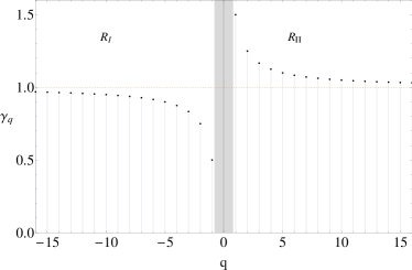
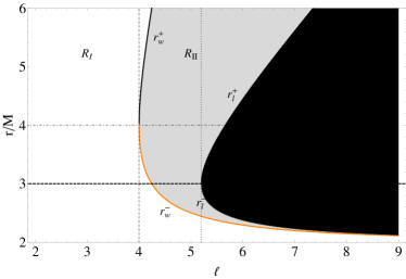
Figure 16: (Color online) Left panel: $\gamma_{q}$ as a function of $q$, where $|q|\geq 1$ are integers. For large values of $|q|$, the index $\gamma$ tends asymptotically to $\gamma=1$. Gray region is forbidden. The maximum value of $\gamma_{q}$ is $\gamma_{q}=3/2$, the minimum is $\gamma_{9}=1/2$. $C<0$ for $V_{sc}^{2}<1$ with $0<\gamma_{q}<1$ in $R_{\mbox{\tiny{I}}}$ and $V_{sc}^{2}>1$ with $\gamma_{q}>1$ in $R_{\mbox{\tiny{II}}}$. Right panel: $r_{l}^{+}$ (black line), $r_{l}^{-}$ (orange line), $r_{W}^{+}$ (thick black line) and $r_{W}^{-}$ (thick orange line) as a function of $\ell$. Dashed line marks $\ell=4$, dotted line $\ell=3\sqrt{3}$, dotted–dashed line $r=r_{mbo}$, thick–dashed line $r=r_{lco}$. White region correspond to the range $R_{\mbox{\tiny{I}}}$, gray region to $R_{\mbox{\tiny{II}}}$.

The condition $C>0$ is satisfied in two cases: where $V_{sc}^{2}<1$ and $\gamma>1$, in the ranges:

$$R_{\mbox{\tiny{I}}}\equiv\left\{\begin{array}[]{lcl}0<\ell<4&\mbox{in}&r>2M\\ \ell\geq 4&\mbox{in}&2M<r<r_{W}^{-}\quad r>r_{W}^{+}\end{array}\right.$$ (80)

and where $V_{sc}^{2}>1$ and $0<\gamma<1$, in the ranges:

$$R_{\mbox{\tiny{II}}}\equiv\left\{\begin{array}[]{lcl}4<\ell<3\sqrt{3}&\mbox{in}&r_{W}^{-}<r<r_{W}^{+}\\ \ell=3\sqrt{3}&\mbox{in}&r_{W}^{-}<r<r_{W}^{+}\quad r\neq r_{lco}\\ \ell>3\sqrt{3}&\mbox{in}&r_{W}^{-}<r<r_{l}^{-}\quad r^{+}_{l}<r<r_{W}^{+}\end{array}\right.$$ (81)

with

$$r_{W}^{\pm}/M\equiv\ell^{2}\pm\frac{\ell}{4}\sqrt{\ell^{2}-16},$$ (82)

(see Fig. 16/ right panel).

We can summarize as follows: when the polytropic index $\gamma=\gamma_{q}$, the fluid density $\rho$ is defined for the conditions $R_{\mbox{\tiny{I}}}\cup R_{\mbox{\tiny{II}}}$, when $\gamma\neq\gamma_{q}$ it is defined only for the conditions $R_{\mbox{\tiny{I}}}$. In the following subsections we will discuss an example of $\gamma=5/3\neq\gamma_{q}$ and the particular case $\gamma_{q}(q=1)=3/2$.

6.1.1 The adiabatic case: $\gamma=5/3$

We consider now the particular case $\gamma=5/3$. This polytropic index is adopted to describe a large variety of matter models, as the generic degenerate matter like star cores of white dwarfs (see e.g. , Horedt2004).

The density $\rho_{\gamma}$ is then:

$$\rho_{5/3}=\left[\left(\frac{r}{r-2M}-\frac{M^{2}\ell^{2}}{r^{2}}\right)^{1/5}-1\right]^{3/2},$$ (83)

defined in the range $R_{\mbox{\tiny{I}}}$ as in Eq. 80:

$$0<\ell<4 r>2M,$$ in (84)

$$\ell\geq 4 2M<r<r^{-}_{W}\;,\;\;r>r^{+}_{W},$$ in (85)

where $\lim_{r\rightarrow r_{W}^{\pm}}\rho_{5/3}=0,$ (see Figs. 17).

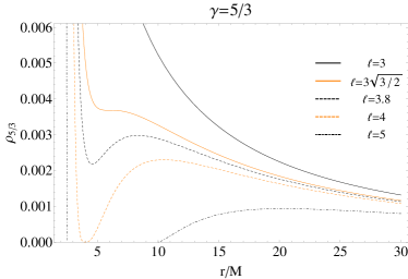
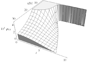
Figure 17: (Color online) Left panel: $\rho_{5/3}$ as a function of $r/M$ for different values of $\ell$. Right panel: $\rho_{5/3}$ as a function of $r/M$ and $\ell$. $\rho_{5/3}$ is not defined in $[r^{-}_{W},r^{+}_{W}]$.

The critical points of $\rho_{5/3}$ can be found as solutions of $\rho^{\prime}_{5/3}=0$:

$$\ell=3\sqrt{{3}/{2}}\quad\mbox{in}\quad r=r_{lsco},\quad 3\sqrt{{3}/{2}}<\ell<4\quad\mbox{in}\quad r=r_{\pm},\quad\ell\geq 4\quad\mbox{in}\quad r=r_{+},$$ (86)

and it is $\rho^{\prime}_{5/3}>0$, (density increasing with the orbital radius) for:

$$3\sqrt{{3}/{2}}<\ell\leq 4\quad\mbox{in}\quad r_{-}<r<r_{+},\quad\ell>4\quad\mbox{in}\quad r_{W}^{+}<r<r_{+}.$$ (87)

We thus conclude that $r_{-}$ is a minimum and $r_{+}$ is a maximum of $\rho_{5/3}$ (see Figs. 18).

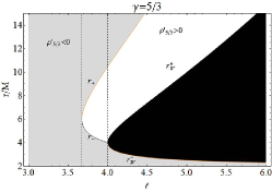
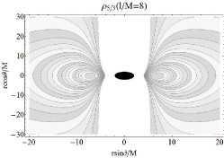
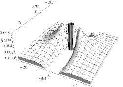
Figure 18: (Color online) Left panel: $r_{W}^{\pm}$ and $r_{\pm}$ as a function of $\ell$. In the gray (white) region $\rho^{\prime}_{5/3}<0$ ($\rho^{\prime}_{5/3}>0$), in the black region $\rho^{\prime}_{5/3}$ is not defined. Central panel: $\rho_{5/3}=\mbox{constant}$ in the plane $(x,y)$. Right panel: $\rho_{5/3}$ as a function of $(x,y)$ for $l=8M$. The black surface is $\sqrt{x^{2}+y^{2}}=2M$.

6.1.2 The case: $\gamma=3/2$

We consider the particular case $\gamma_{q}(q=1)=3/2$, which is in the extreme cases $1<\gamma<5/3$.

The density $\rho_{3/2}\neq 0$ is then:

$$\rho_{3/2}=\left[\left(\frac{r}{r-2M}-\frac{M^{2}\ell^{2}}{r^{2}}\right)^{1/6}-1\right]^{2},$$ (88)

defined in the range $R_{\mbox{\tiny{I}}}\cup R_{\mbox{\tiny{II}}}$ as in Eqs. 80-81:

$$0<\ell<4 r>2M,$$ in (89)

$$4\leq\ell<3\sqrt{3} r>2M,\quad r\neq r_{W}^{\pm}$$ in (90)

$$\ell\geq 3\sqrt{3} 2M<r<r_{l}^{-},\quad r>r_{l}^{+}\quad r\neq r_{W}^{\pm},$$ in (91)

where $\lim_{r\rightarrow r_{W}^{\pm}}\rho_{3/2}=0,$ (see Figs. 19).

The critical points of $\rho_{3/2}$ can be found as solutions of $\rho^{\prime}_{3/2}=0$, or noting that $p^{\prime}=\frac{3}{2}\rho^{\prime}\sqrt{\rho}$. We summarize these results concluding that $r_{-}$ is a minimum and $r_{+}$ is a maximum of $\rho_{3/2}$.

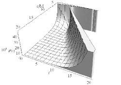
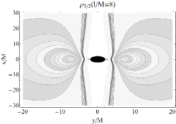
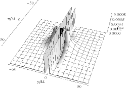
Figure 19: Left panel:$\rho_{3/2}$ as a function of $r/M$ and $\ell$. $\rho_{3/2}$ is not defined in $[r^{-}_{l},r^{+}_{l}]$. Central panel: $\rho_{5/3}=\mbox{constant}$ in the plane $(x,y)$. Right panel: $\rho_{3/2}$ as a function of $(x,y)$ for $l=4M$. The black surface is $\sqrt{x^{2}+y^{2}}=2M$.

6.2 The isothermal case: $\gamma=1$

For an isothermal equation of state $(\gamma=1)$, the solution of Eq. 74 is $\rho=\rho_{k}$ (see Eq. 75). This function is not defined in the range $r_{l}^{-}\leq r\leq r_{l}^{+}$ and the fluid angular momentum is $0<\ell<\ell_{r}$.

In order to describe the regions of maximum and minimum density, we study the function $\rho_{k}^{\prime}$. Being $p=k\rho$, it is clearly $p^{\prime}=k\rho^{\prime}$. Thus it is $\rho^{\prime}=0$ when $p^{\prime}=0$. Moreover, being $k>0$, the maxima (minima) of $p$ correspond to maxima (minima) of $\rho$. The existence of critical points for the isothermal case is therefore studied in Sect. 3.3 in terms of the critical points of $G_{r}$:

$$\ell=3\sqrt{{3}/{2}}\quad\mbox{in}\quad r=r_{lsco},\quad 3\sqrt{{3}/{2}}<\ell<3\sqrt{3}\quad\mbox{in}\quad r=r_{\pm},\quad\ell\geq 3\sqrt{3}\quad\mbox{in}\quad r=r_{+},$$ (92)

or also $r>r_{lco}\quad\ell=\ell_{\rm{\rm{K}}}.$

7 The fluid proper angular velocity

This Section concerns with the analysis of the fluid velocity field, in particular we are interested in assessing the orbits and the plans where the fluid proper velocity is maximum or minimum.

The fluid four velocity along the $\varphi$ angular direction is:

$$\Phi=\frac{L}{r^{2}\sigma^{2}}=\frac{1}{\sigma^{2}r^{2}}\sqrt{\frac{\sigma^{2}l^{2}(r-2M)r^{2}}{\sigma^{2}r^{3}-l^{2}(r-2M)}}\,,$$ (93)

where we are always considering $L>0$ and $\Phi>0$. We redefine $\Phi$ as a dimensionless quantity:

$$\frac{\Phi\sigma^{2}}{M}=\frac{M^{2}}{r^{2}}\sqrt{\frac{\ell^{2}(r-2M)r^{2}}{r^{3}-\ell^{2}M^{2}(r-2M)}}\,.$$ (94)

Clearly it is $\Phi\gtreqless 0$ when $L\gtreqless 0$, and they have the same existence conditions ($0<l<l_{r}$, $2M<r<r_{l}^{-}$ and $r>r_{l}^{+}$). The behavior of the angular velocity as a function of $\sigma$, $l$, and $r$ are portrayed in Figs. 20.

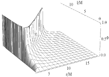
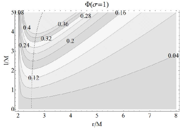
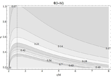
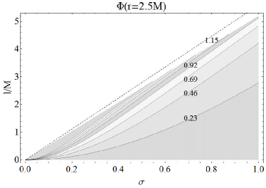
Figure 20: Upper left panel: $\Phi=aU^{\varphi}/M$ on the equatorial plane $\sigma=1$ as a function of $r/M$ and $l/M$. The function is defined for $l\in[0,l_{r}]$. Upper right panel: $\Phi=\mbox{constant}$ as function of $l/M$ and $r/M$ on the equatorial plane $\sigma=1$. The curves have minima in $r=r_{\chi}$. Lower left panel: $\Phi=\mbox{constant}$ in the plane $\sigma$ and $r/M$ for $l/M=1$. The curves have maxima in $r=5/2M$ (dashed line). Lower right panel: $\Phi=\mbox{constant}$ in the plane $\sigma$ and $\ell$ for $r/M=5/2$. No motion is allowed for $\ell>\ell_{r}$ ($\ell=\ell_{r}$, dashed line), and it is $\Phi^{\prime}=0$ on $r=r_{\chi}^{-}$, $l=l_{\chi}$ and $\sigma=\sigma_{\chi}$.

In order to derive the critical points of the proper angular velocity as a function of $r$, we consider the solutions of the equation $\Phi^{\prime}=0$. Apart from the trivial case $l=0$ and $\Phi=0$, the proper angular velocity is constant with respect to the radial coordinate when:

$$l=l_{\chi}\equiv\sqrt{\frac{\sigma^{2}r^{3}(2r-5M)}{(r-2M)^{2}}}\quad\mbox{for}\quad{5}/{2}M<r<3M,$$ (95)

where $0<l_{\chi}<3\sqrt{3}M$. In terms of the angular momentum and the radius, the orbits of $\Phi$ belong to the planes:

$$\sigma=\sigma_{\chi}\equiv l\sqrt{\frac{(r-2M)^{2}}{r^{3}(2r-5M)}}\quad\mbox{for}\quad r_{\chi}<r<r_{lco}\quad(\sigma=1\quad\mbox{when}\quad r=r_{\chi})\,,$$ (96)

where:

$$r_{\chi}=r^{\pm}_{\chi}/M \equiv \frac{5}{8}+\frac{1}{2}\sqrt{\frac{25}{8}+\frac{2\ell^{2}}{3}-\frac{\ell^{2}\left(\ell^{2}-36\right)}{6\alpha}-\frac{\alpha}{6}\mp\frac{\sqrt{3}\left(\frac{125}{8}-11\ell^{2}\right)}{\beta}}\mp\frac{\beta}{8\sqrt{3}},$$ (97)

with

$$\alpha \equiv \left[-\ell^{2}\left(\ell^{4}-54\ell^{2}+1350-6\sqrt{48\ell^{4}-2754\ell^{2}+50625}\right)\right]^{1/3},$$ (98)

$$\beta \equiv \sqrt{16\ell^{2}+75+\frac{8\ell^{2}\left(\ell^{2}-36\right)}{\alpha}+8\alpha}\ .$$ (99)

As shown in Figs. 21, $2.5M<r_{\chi}<3M$ and the orbital radius $r_{\chi}$ increases with ${\ell=l/(M\sigma)}$. An alternative analysis of the proper fluid angular velocity, as function of ${(l,r,\sigma)}$, is presented in Appendix  B.

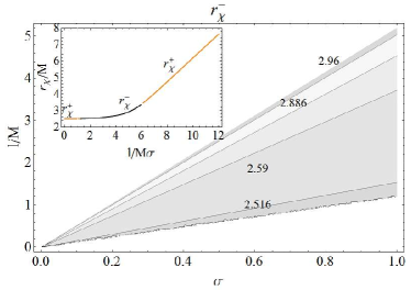
Figure 21: (Color online)Left panel: $r^{-}_{\chi}=$constant as a function of $0<\sigma<1$ and $0<l/M<3\sqrt{3}$. Inset $r^{-}_{\chi}$ (black line) and $r^{+}_{\chi}$ (orange line) as increasing functions of $\ell=l/(\sigma M)$. Right panel: $r^{+}_{\chi}/M$ (orange line) and $r^{-}_{\chi}/M$ (black line) as a function of $\sigma$. Gray region corresponds to $r\in[r_{lco},\infty]$. Dotted lines mark $\sigma=\sigma_{l}$ for the selected $l/M$.

8 Comparing the fluid relativistic angular velocity and the Keplerian angular momentum

In this Section we compare the fluid configurations with $\partial_{r}p\neq 0$ with the model $p=$constant where the disk is geodetic by studying the relativistic angular velocity and comparing our results with the Keplerian definitions. In Sect. 3.2 we already explored the fluid behavior with respect to $l_{\mbox{\tiny{K}}}$. We summarize here the results considering the ratio:

$$\Pi_{\mbox{\tiny{LK}}}\equiv L/L_{\mbox{\tiny{K}}}=\Phi/\Phi_{\mbox{\tiny{K}}}=\sqrt{\frac{\ell^{2}M(r-3M)(r-2M)}{r^{3}-\ell^{2}M^{2}(r-2M)}}\,,$$ (100)

which is defined for $0<\ell\leq 3\sqrt{3}$ in $r>r_{lco}$, and for $\ell>3\sqrt{3}$ in $r>r^{+}_{l}$. The regions where $L(l)$ is larger or smaller than $L_{\mbox{\tiny{K}}}=L(l_{\mbox{\tiny{K}}})$ for different values of the fluid constant of motion $l$ are portrayed in Figs. 22 upper left panel. We have $\lim_{r\rightarrow\infty}\Pi_{\mbox{\tiny{LK}}}=\lim_{r\rightarrow r_{lco}}\Pi_{\mbox{\tiny{LK}}}=0$. In general, $L>L_{\mbox{\tiny{K}}}$ for fluid angular momentum $l$ sufficiently large, for $l$ sufficiently low or far from the source it is $L<L_{\mbox{\tiny{K}}}$ (see Figs. 22 upper left panel).

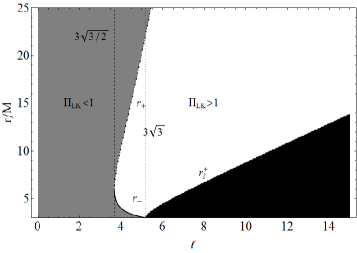
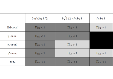
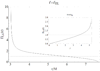
Figure 22: Upper left panel: $r_{\pm}$ and $r^{+}_{l}$ as a function of $\ell$. $\Pi_{\mbox{\tiny{LK}}}$ is not defined in the black region. $\Pi_{\mbox{\tiny{LK}}}>1$ in the white region and $\Pi_{\mbox{\tiny{LK}}}<1$ in the gray region. Dashed line marks $\ell=3\sqrt{3/2}$, dotted line $\ell=3\sqrt{3}$. Upper right panel: $r_{\Pi_{LK}}$, $r^{+}_{l}$, $r_{\pm}$ as a function of $\ell$. $\Pi_{\mbox{\tiny{LK}}}$ is not defined in $r<r^{+}_{l}$ (black region). For $r<r_{\Pi_{LK}}$ it is $\Pi^{\prime}_{\mbox{\tiny{LK}}}>0$ (white region). The gray colored region corresponds to $\Pi^{\prime}_{\mbox{\tiny{LK}}}<0$. When $r=r_{\pm}$ it is $\Pi_{\mbox{\tiny{LK}}}=1$. Dashed thin line marks $\ell=3\sqrt{3}$. Lower left panel: table summarizing the regions $\Pi_{\mbox{\tiny{LK}}}>1$ (light-gray regions) and $\Pi_{\mbox{\tiny{LK}}}<1$ (gray regions) for different values of $r/M$ and $\ell$. $\Pi_{\mbox{\tiny{LK}}}$ is not defined in the black boxes. Lower right panel : $\Pi_{\mbox{\tiny{LK}}}(\ell_{\Pi_{LK}})$ as a function of $r/M\in[3.76,7.88]$. Dashed line marks $\Pi_{\mbox{\tiny{LK}}}=1$. Inset: $\Pi_{\mbox{\tiny{LK}}}(r_{\Pi_{LK}})$ as a function of $\ell\in[0,3\sqrt{3}]$. Dashed line marks $\Pi_{\mbox{\tiny{LK}}}=1$.

We are now interested to define the critical points of the ratio $\Pi_{\mbox{\tiny{LK}}}$. The solutions of the equation $\Pi^{\prime}_{\mbox{\tiny{LK}}}=0$ are, in terms of the angular momentum:

$$\ell_{\Pi_{LK}}\equiv\frac{r\sqrt{(10M-r)r-18M^{2}}}{M(r-2M)}\,,$$ (101)

and in terms of the orbital radius:

$$r_{\Pi_{LK}}/M=\frac{1}{6}\left[15+\sqrt{3}\sqrt{78-4\ell^{2}-\frac{\left(\ell^{2}-18\right)^{2}}{\kappa}-\kappa^{1/3}-\frac{6\sqrt{3}\left(\ell^{2}-35\right)}{\bar{\kappa}}}+\sqrt{3}\bar{\kappa}\right]\,,$$ (102)

with

$$\kappa \equiv \left[54\left(108+10\ell^{2}-\ell^{4}\right)+\ell^{6}+12\sqrt{6}\sqrt{-\ell^{2}\left(\ell^{2}-27\right)\left(\ell^{4}-54\ell^{2}+756\right)}\right]^{1/3}\,,$$ (103)

$$\bar{\kappa} \equiv \sqrt{\frac{\ell^{4}-2\ell^{2}(18+\kappa)+(12+\kappa)(27+\kappa)}{\kappa}}\,.$$ (104)

These are defined for $r_{lco}<r_{\Pi_{LK}}<(5+\sqrt{7})$ and $0<l_{\Pi_{LK}}<3\sqrt{3}$. The sign of $\Pi^{\prime}_{\mbox{\tiny{LK}}}$ as a function of $r$ and $l$ is summarized in Fig. 22, upper right panel. In particular, it is manifest that $r_{\Pi_{LK}}$ is a maximum of $\Pi_{\mbox{\tiny{LK}}}$. The values of this maximum, $\Pi_{\Pi_{LK}}(\ell)=\Pi_{\mbox{\tiny{LK}}}(\ell=\ell_{\Pi_{LK}})$ and $\Pi_{\Pi_{LK}}(r)=\Pi_{\mbox{\tiny{LK}}}(r=r_{\Pi_{LK}})$, are portrayed in Fig. 22, lower right panel. We note in particular that $\Pi_{LK}$ is an increasing function of $l$: this implies that the larger the angular momentum of fluid, the larger is the ratio between $L$ and the angular momentum of the free particle $L_{K}$.

8.1 The fluid relativistic angular velocity $\Omega$: the Von Zeipel surfaces

The fluid relativistic angular velocity $\Omega$ is:

$$\Omega\equiv\frac{\Phi}{\Sigma}\equiv-l\frac{g_{tt}}{g_{\varphi\varphi}}=\frac{l(r-2M)}{r^{3}\sigma^{2}}=\frac{l}{l_{r}^{2}},$$ (105)

The function ${\Omega=\sigma\Omega(\ell)}$:

$$\Omega=\frac{\ell M(r-2M)}{r^{3}}$$ (106)

is defined in $r>2M$, and has a maximum in $r=r_{lco}$ (see Fig. 23, left panel).

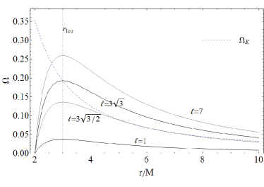
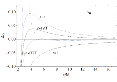
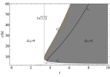
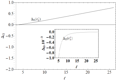
Figure 23: (Color online) Upper left panel: the relativistic angular velocity $\Omega$ in units of $1/M$, for $\sigma=1$ as a function of $r/M$, for different values of $\ell$. Dashed line marks the Keplerian velocity $\Omega_{\mbox{\tiny{K}}}$. Dotted line marks $r=r_{lco}=3M$, a maximum of $\Omega$. For $\ell=3\sqrt{3/2}$, it is $\Omega=\Omega_{\mbox{\tiny{K}}}$ in $r=r_{lco}=3M$; for $\ell=3\sqrt{3}$, it is $\Omega=\Omega_{\mbox{\tiny{K}}}$ in $r=r_{lsco}=6M$ and in $r=6(2+\sqrt{3})M$. Upper right panel: $\Delta_{\Omega}$ as a function of $r/M$, for different values of $\ell$. Dashed line marks the maximum of $\Delta_{\Omega}$. Lower left panel: $r_{o}^{\pm}$ and $r_{\pm}$ as a function of $\ell$. In the white (gray) regions it is $\Delta^{\prime}_{\Omega}>0$ ($\Delta^{\prime}_{\Omega}<0$). $\Delta_{\Omega}=0$ when $r=r_{\pm}$, and $\Delta_{\Omega}$ is maximum in $r={r}_{o}^{-}$ and minimum in $r={r}_{o}^{+}$. Lower right panel: $\Delta_{\Omega}(r_{o}^{-})$ as a function of $\ell$. Inset: $\Delta_{\Omega}(r_{o}^{+})$ as a function of $\ell$.

The surfaces known as the von Zeipel’s cylinders, are defined by the conditions: $l=\mbox{constant}$ and $\Omega=\mbox{constant}$ (see for example , Abramowicz1971, Chakrabarti1991, Chakrabarti1990). In the static spacetimes the family of von Zeipel’s surfaces does not depend on the particular rotation law of the fluid, $\Omega=\Omega(l)$, in the sense that it does not depend on nothing but the background spacetime. In the case of a barotropic fluid, the von Zeipel’s theorem guarantees that the surfaces $\Omega=\mbox{constant}$ coincide with the surface with constant angular momentum. More precisely, the von Zeipel condition states: the surfaces at constant pressure coincide with the surfaces of constant density (i.e. the isobar surfaces are also isocore) if and only if the surfaces with the angular momentum $l=\mbox{constant}$ coincide with the surfaces with constant angular relativistic velocity (, Kozłowski et al.1978, Jaroszynski et al.1980, Abramowicz1971, Chakrabarti1991, Chakrabarti1990).

The surfaces $\Omega/l=s>0$, being $s$ a constant, are defined by:

$$r_{s}^{-}/M \equiv -\frac{2\sqrt{\frac{M^{2}}{\sigma^{2}s}}\cos\left[\frac{1}{3}\left(\pi+\arccos\left[-\frac{3\sqrt{3}}{\sqrt{\frac{M^{2}}{\sigma^{2}s}}}\right]\right)\right]}{\sqrt{3}},\quad r_{s}^{+}/M\equiv\frac{2\sqrt{\frac{M^{2}}{\sigma^{2}s}}\cos\left[\frac{1}{3}\arccos\left(-\frac{3\sqrt{3}}{\sqrt{\frac{M^{2}}{\sigma^{2}s}}}\right)\right]}{\sqrt{3}}.$$ (107)

These are a function of the product $\sigma^{2}s$, and they exist for $0<\sigma^{2}s\leq(1/27)M^{2}$. In particular, $\sigma^{2}s=(1/27)M^{2}$ corresponds to $r_{s}^{\pm}=r_{lco}$ (see Fig. 24, upper left panel). In the $(x,y)$ coordinates, the $\Omega/l=s>0$ surfaces read:

$$x_{s}^{\pm}\equiv\pm\sqrt{\left(\frac{2M^{5}}{M^{4}-sy^{2}}\right)^{2}-y^{2}}$$ (108)

(see Figs. 24).

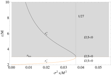
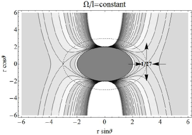
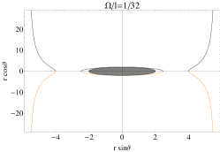
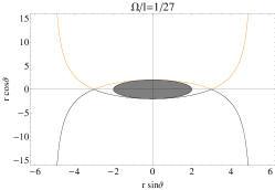
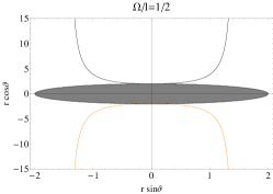
Figure 24: (Color online) Upper left panel: $r_{s}^{\pm}/M$ as a function of $(\sigma^{2}s)$. Dashed lines mark the conditions $r=r_{lco}$, $\sigma^{2}s=(1/27)M^{2}$. The white region $(r<r_{lco})$ corresponds to $\Omega^{\prime}/l>0$, the light-gray region $(r>r_{lco})$ to $\Omega^{\prime}/l<0$. $\Omega^{\prime}/l=0$ in $r=r_{lco}$. Upper right panel: surfaces $\Omega/l=s$ with $r/M=\mbox{constant}$ in coordinate $x=r\cos{\vartheta}$, $y=r\sin{\vartheta}$. The surface $s=(1/27)M^{2}$ is marked with a number. The gray region marks the circle $r\leq 2M$. Arrows follow the increasing (decreasing) direction respect of $s$. Lower panels: surfaces $\Omega/l=s$ in units of $M^{2}$ as a function of $x=r\cos{\vartheta}$, $y=r\sin{\vartheta}$ in units of $M$, for different values of $s$. The gray region underlines the circle $r\leq 2M$. Dashed circle corresponds to $r=r_{lco}$.

We are now interested in characterizing the angular velocity with respect to the Keplerian velocity $\Omega_{\mbox{\tiny{K}}}\equiv\frac{\sqrt{M}}{\sigma r^{3/2}}$. We therefore consider the dimensionless difference $\mathbf{\Delta_{\Omega}\equiv(\Omega-\Omega_{\mbox{\tiny{K}}})M\sigma}$:

$$\mathbf{\Delta_{\Omega}=M\sigma\frac{\ell M(r-2M)-\sqrt{r^{3}M}}{\sigma r^{3}}.}$$ (109)

$\Delta_{\Omega}=0$ for $r\rightarrow\infty$, $\Delta_{\Omega}(r=2M)=-1/2\sqrt{2}$, $\Delta_{\Omega}(r_{lco})=\left(\ell-3\sqrt{3}\right)/27$, and $\Delta_{\Omega}(r_{lsco})=\left(2\ell-3\sqrt{6}\right)/108$ (see Fig. 23, right panel). $\Delta_{\Omega}(r=2M)$ is negative irrespective of the value of $\ell$. The sign of $\Delta_{\Omega}(r_{lco})$ and $\Delta_{\Omega}(r_{lsco})$, on the contrary, depends on the fluid angular momentum. The sign of $\Delta_{\Omega}$ as a function of $r$ and $\ell$ is summarized in Figs. 25.

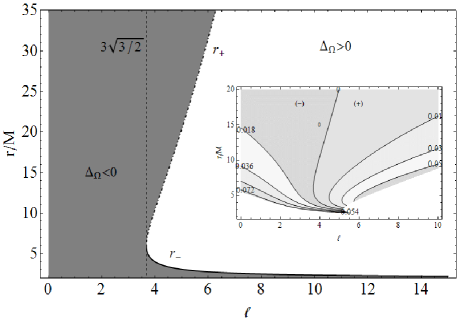
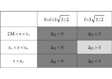
Figure 25: Upper panel: $r_{\pm}$ as a function of $\ell$. Gray region corresponds to $\Delta_{\Omega}<0$, white region to $\Delta_{\Omega}>0$. $\Delta_{\Omega}=0$ in $r=r_{\pm}$. Inset: curves $\Delta_{\Omega}=\rm{constant}$. The regions of positive and negative $\Delta_{\Omega}$ are underlined. Lower panel: table summarizing the regions $\Delta_{\Omega}>0$ (light-gray) and $\Delta_{\Omega}<0$ (gray).

The difference $\Delta_{\Omega}$ is maximum in $r>r_{lco}$ when $\ell=(3/4)\ell_{\mbox{\tiny{K}}}$. Notably, $\ell_{\mbox{\tiny{K}}}$ is not a critical point of the angular velocity difference $\Delta_{\Omega}$. $\Delta_{\Omega}$ always increases in $2M<r\leq r_{lco}$ for all $\ell$, and for $0<\ell<(3/4)\ell_{\mbox{\tiny{K}}}$ in the region $r>r_{lco}$. Other critical points are for $\ell\geq 27/8$ in $r=r^{\pm}_{o}$:

$$r_{o}^{-}/M \equiv \frac{8}{27}\left(2\ell^{2}-\sqrt{2}\sqrt{\ell^{2}\left(8\ell^{2}-81\right)}\cos\left[\frac{1}{3}\left(\pi+\arccos\hat{o}\right)\right]\right),$$ (110)

$$r_{o}^{+}/M \equiv \frac{8}{27}\left(2\ell^{2}+\sqrt{2}\sqrt{\ell^{2}\left(8\ell^{2}-81\right)}\cos\left[\frac{1}{3}\arccos\hat{o}\right]\right),$$ (111)

with

$$\hat{o}\equiv\frac{\ell^{2}\left(512\ell^{4}-7776\ell^{2}+19683\right)}{16\sqrt{2}\left[\ell^{2}\left(-8\ell^{2}-81\right)\right]^{3/2}},$$ (112)

where $r_{o}^{-}=r_{o}^{+}=9M$ for $\ell=27/8$. $\Delta_{\Omega}$ always increases in $0<\ell<27/8$, and for $\ell\geq 27/8$ in the regions $(2M,r_{o}^{-})$ and $r>r_{o}^{+}$, while it decreases in $\ell\geq 27/8$ in the region $(r_{o}^{-},r_{o}^{+})$. The radius $r_{o}^{+}$ is a minimum and $r_{o}^{-}$ a maximum point of $\Delta_{\Omega}$. The critical points values $\Delta_{\Omega}(r_{o}^{\pm})$ are portrayed in Figs. 23, lower panels.

We analyze the profile of the proper angular velocity, $\Phi$, and the relativistic angular velocity, $\Omega$, respect to the corresponding Keplerian quantities for the case of a isothermal matter. Clearly, with respect to the general analysis, here we should take into account the specific density and pressure profile emerging by the choice of the particular equation of state, $p=k\rho^{\gamma}$.

9 Summary and conclusions

The analysis of a stationary axisymmetric configuration of material, in equilibrium in a Schwarzschild spacetime, as emerging in the Polish doughnut framework constitutes a timely question in view of the interest in astrophysical sources, possibly resulting from super-Eddington accretion onto very compact objects, like Gamma-Ray Bursts, Active Galactic Nuclei, binary systems and Ultraluminous X-ray sources (see e.g. , Fender& Belloni2004, Soria2007). The most characterizing features of the Polish doughnut approach is the thickness of the matter distribution across the equilibrium and the existence of a region enveloping the horizon surface, where the fluid can, in principle, infall onto the black hole. The first property is of impact for a comparison with the wide spectrum of numerical simulation of a thick disk (see Straub et al.2012, Font2003, Abramowicz& Fragile2011 for recent examples). The non-negligible depth of the accreting profile is typical of the regime where the gravitational effects are strong and it takes a relevant role in all those extreme phenomena associated with the gravitational collapse, characterized by a violent energy-matter release from the central compact object. The second aspect is relevant because the Polish doughnut model can account for a non-zero accretion rate of the torus even when the dissipative effects are negligible. This is in contrast to the original idea by (Shakura & Sunyaev1973) that the angular momentum transport is always allowed by the shear viscosity of the accreting material. Indeed, the accreting plasma is in general quasi-ideal and the emergence of dissipative effects as those required to match the observations requires the appearance in the dynamics of a strong turbulent regime, restated as a laminar one in the presence of a significant shear viscosity. Since this picture is not yet settled down (see , Balbus2011), it is very important that an ideal hydrodynamical scheme on a Schwarzschild background like the one offered by the Polish doughnut is able to account for a material infalling onto a black hole.

In this work we revisited the Polish doughnut model of accretion disks for a perfect fluid circularly orbiting around a Schwarzschild black hole with the effective potential approach for the exact gravitational and centrifugal contributions. We take advantage of the formal analogy between the fluid when the pressure vanishes and the test particle orbiting in the same background to get a comparison between the Polish doughnut, which is supported by the pressure, and the geodetic disk. Our analysis provides a revisited theoretical framework to characterize the accretion processes in presence of general relativistic effects. Indeed we formulate the Polish doughnut model in such a way that the fluid dynamics can be interpreted in terms of the fundamental stability properties of the circular orbits in Schwarzschild background.

We extensively analyzed the Polish doughnut configurations for the fluid $l$ and the particle $L$ angular momenta, taken respectively constant throughout the entire toroidal surface. Then we propose a reinterpretation of torus physics, with respect to the its shape and equilibrium dynamics in terms of the parameter $l$ (and $L$), and in terms of the parameter $K$ that was naturally established by introducing the effective potential for the fluid motion. This new parameter $K$ has been derived by exploiting the methodological and formal analogy with the effective potential approach to the test particles motion. Note that ($l$, $K$) fully describe the toroidal fluid configuration. This procedure made it possible to emphasize the pressure influence in the equilibrium dynamics with respect to the case of dust, the latter being treated as a set of test particles not subjected to pressure. This dual aspect, methodological and procedural, we thought it required a complete and deep analysis of the behavior of the momenta $l$ and $L$ on the plans and disk orbits, and of $L$ as a function of $l$, and of the surface characteristic parameters as a function of $K$.

The main steps of this analysis are:

Radial pressure gradient vs angular momentum $\mathcal{L}$

We studied the pressure radial gradient as a function of $r$ and of the angular momentum $\mathcal{L}$. The pressure is a decreasing function of $r$ in $r<r_{lco}$. and for $\mathcal{L}<\mathcal{L}_{K}$ it is $p^{\prime}<0$, this means that $\mathcal{L}_{K}$ identifies the pressure minimum points located in $[r_{lco},r_{lsco}]$, and pressure maximum points in $r>r_{lsco}$ (see Fig. 1, right panel). However, at fixed orbit $r$, $\mathcal{L}_{K}$ is always a minimum point of $r$ ie at fixed $r$ the pressure decreases until the angular momentum reaches the values $\mathcal{L}=\mathcal{L}_{K}$, and then increases with $\mathcal{L}$ (note that $r_{lsco}$ is a minimum point of $\mathcal{L}_{K}$).

Angular momentum $\mathcal{L}$ vs. fluid angular momentum $\ell$

We found that at fixed $\ell$ the angular momentum $\mathcal{L}(r,l)$ has a maximum for $r=r_{-}\in[r_{lco},r_{lsco}]$, and a minimum in $r_{+}>r_{lsco}$, and $\mathcal{L}(r)$ increases for $r<r_{-}$ and $r>r_{+}$ (Fig. 3). We identify three possibilities: $\ell<3\sqrt{3/2}$, where the momentum $\mathcal{L}(r)$ increases with $r$; $3\sqrt{3/2}<\ell<3\sqrt{3}$, where $\mathcal{L}$ increases with $r$ up to the maximum point $r_{-}$, decreases up to the minimum $r_{+}$; $\ell>3\sqrt{3}$, where $\mathcal{L}$ increases with $r$.

Pressure gradients vs fluid angular momentum $\ell$

The fluid pressure decreases for $r<r_{l}^{-}$ and $r>r_{+}$ as well as for $\ell<3\sqrt{3/2}$ (Fig. 4). The situation is much more complicated for fluid with higher angular momenta ($\ell>3\sqrt{3/2}$). It appears necessary to consider fluids with $3\sqrt{3/2}<\ell<3\sqrt{3}$ and with $\ell>3\sqrt{3}$ separately. In the first case we observe the presence of a ring $[r_{-},r_{+}]$ where the fluid pressure increases with the orbital radius, $r_{-}$ being a pressure minimum and $r_{+}$ a pressure maximum. In the case $\ell>3\sqrt{3}$ we find two rings, $[r_{l}^{-},r_{-}]$ and $[r_{l}^{+},r_{+}]$, where the fluid pressure is an increasing function of $r$. Figure 4 upper right describes this situation from a different point of view: for what concerns the variation of its hydrodynamic pressure with the orbits and the angular momentum, the fluid dynamics is basically split into two zones, $r<r_{lco}$ and $r>r_{lco}$, respectively: in the first region, the fluid pressure decreases with increasing angular momentum up to $\ell=\ell_{r}$ (minimum), then it increases with $\ell$ up to $\ell_{K}$ (maximum), finally it decreases with $\ell$. The trend is precisely the same in the region $r>r_{lco}$, but $\ell_{k}$ and $\ell_{r}$ are now the minimum and maxima momentum respectively, i.e. the fluid pressure decreases with $\ell<\ell_{k}$, grows in the range $[\ell_{k},\ell_{r}]$ and then decreases with $\ell$. The angular pressure gradient has been studied and compared to the radial and angular gradient in Sec. 4.

The Boyer surfaces and polytropic equation of state

In Sec. 5 we drew a complete and analytic description of the toroidal surface of the disk. A key role of this analysis was played by the effective potential approach: the toroidal disk can be described once one gives the effective potential and the fluid angular momentum. Our results concerning the disk shape and structure can be summarized as follows:

1. the distance from the source of the torus inner surface ($\delta=y_{2}-2M$), increases with increasing angular momentum of the fluid but decreases with increasing energy function defined as the value of the effective potential for that momentum;

2. the surface maximum height (torus thickness - $h$), increases with the energy and decreases with the angular momentum:the torus becomes thinner for high angular momenta, and thicker for high energies;

3. the location of maximum thickness of the torus moves towards the external regions with increasing angular momentum and energy, until it reaches a maximum an then decreases;

4. the surface maximum diameter $(\lambda)$ increases with the energy, but decreases with the fluid angular momentum;

5. the distance of the torus inner surface from the structure inner surface $(\hat{\delta}=y_{2}-y_{1})$ increases with the angular momentum and decreases with the energy;

6. the distance of the structure inner surface from the horizon ($\breve{\delta}\equiv y_{1}-2M$) increases with the energy and decreases with the fluid angular momentum.

The accreting fluids with a polytropic equation of state were studied in the Section 6, divided into two classes identified by their polytropic index.

The fluid angular velocity

In Section 7 we analyzed the fluid proper angular velocity $\Phi$ and we have compared the proper velocity with the Keplerian one $\Phi_{K}$ in Section 8: the velocity $\Phi<\Phi_{K}$ in $r>r_{+}$ and for all $r$ when $\ell<3\sqrt{3/2}$ (see Fig. 22). As for the analysis of the angular momentum $L(r,l)$, a distinction is made between fluids with $\ell\in[3\sqrt{3/2},3\sqrt{3}]$, characterized by a ring $[r_{-},r_{+}]$ where the proper velocity is higher then the kepler one, and fluids with $\ell>3\sqrt{3}$, where the proper fluid velocity is greater than the Keplerian one in the inner regions, $r<r_{-}$. Finally, we have investigated the regions and momenta where the difference $\Phi-\Phi_{K}$ is maximum (see Fig. 22). We concluded the study of velocity fields by analyzing the fluid relativistic velocity $\Omega$ and the Von Zeipel surfaces in Section 8. The velocity $\Omega$ has a maximum at $r_{lco}$ and increases with the increasing of $\ell$. We also studied the differences $\Delta_{\Omega}\equiv(\Omega-\Omega_{\mbox{\tiny{K}}})M\sigma$ between the relativistic fluid velocity and the Keplerian one $\Omega_{\mbox{\tiny{K}}}$ (see Fig. 23). At fixed angular momentum $\ell>3\sqrt{3/2}$, this difference has a maximum and a minimum, while for $\ell<3\sqrt{3/2}$ it is always decreasing. The fluid velocity $\Omega$ is lower then the Keplerian $\Omega_{K}$ for $r<r_{-}$ and $r>r_{+}$, and for any $r$ when $\ell<3\sqrt{3/2}$, instead for fluid with with angular momentum greater then $\ell=3\sqrt{3/2}$ there is a ring $[r_{-},r_{+}]$ where the fluid velocity $\Omega$ is larger then the Keplerian one (see Fig. 25).

The fundamental merit of the present work is that the analysis of the Polish doughnut features maintain the explicit presence of the effective potential in all the basic expressions describing the matter distribution. In fact, this allows to keep in direct contact our study with the behavior of free test particles moving the gravitational field of the central object and following circular orbit (the dust, pressure-free limit of the present analysis). What is significant here is the possibility to compare configuration of the considered fluid, as described by certain values of the parameters $K$ and $l$, with the behavior of the test particle system, characterized by the same values of the corresponding parameters $K$ and $L$. These latter quantities have a precise meaning for the particle (energy and angular momentum as viewed at infinite distance), while the corresponding parameters for the fluid must, on this level, regarded as a classification criterion for the torus morphology. Thus retaining the effective potential in the Polish doughnut treatment allows to identify the Boyer surfaces in terms of parameters that have a precise meaning for a different, but closely related, context, the pressure-free fluid, i.e. the fundamental features of the Schwarzschild spacetime. If this study can not yet directly offer a paradigm for the comparison with the observations, nonetheless, it makes a concrete step in this direction. We are now able to constrain the morphology of the equilibrium configuration by fixing the two parameters $K$ and $l$, i.e. specifying their value, we can define the basic features of the torus shape and of the velocity field in different space regions (this is synthetically sketched in the ten final remarks, achieved by our systematic analysis) and the comparison with the corresponding profile of the particle motion, where the physical comprehension is settled down, offer a valuable tool to interpret what the observations trace out. Our model will be completed including other relevant ingredients, like dissipative effects and the magnetic field and this is probably the natural development of the conceptual paradigm we fixed here.

Appendix A The radial gradient $G_{r}$ as function of $\sigma$.

In Section 3.1 and  3.3 we detailed the study of the radial gradient $G_{r}$ as a function of the angular momentum $L$ and of the fluid angular momentum $l$ with a re-parametrization that is independent from the equatorial plane $\sigma$. However, an explicit study of $G_{r}$ as a function of $\sigma$ is useful for two main reasons: first, to have a direct comparison when the re-parametrization is not possible (as for the polar gradient $G_{\vartheta}$). Secondly, the angular dependence is necessary to build a three-dimensional characterization of the torus.

In Section 3 we showed that the critical points of the pressure are defined by the condition Eq. 14. In terms of the polar coordinate, it reads:

$$\sigma_{\mbox{\tiny{K}}}^{\mbox{\tiny{L}}}\equiv\frac{L}{M}\sqrt{\frac{M(r-3M)}{r^{2}}}\,.$$ (113)

The condition of existence of $\sigma_{\mbox{\tiny{K}}}^{\mbox{\tiny{L}}}$ are $r>r_{lco}$ for $0<L\leq 2\sqrt{3}M$, and $r_{lco}<r\leq r_{\mbox{\tiny{L}}}^{-}(\sigma=1)$ and $r\geq r_{\mbox{\tiny{L}}}^{+}(\sigma=1)$ for $L>2\sqrt{3}M$, where $r_{\mbox{\tiny{L}}}^{+}(\sigma=1)$ are the circular orbit radii for a test particle in Schwarzschild spacetime defined by Eq. 15, evaluated at $\sigma=1$. The point $r_{lsco}$ is a maximum for $\sigma_{\mbox{\tiny{K}}}^{\mbox{\tiny{L}}}$: the condition $r_{\mbox{\tiny{L}}}^{+}=r_{\mbox{\tiny{L}}}^{-}=r_{lsco}$ is fulfilled when $\sigma_{\mbox{\tiny{K}}}^{\mbox{\tiny{L}}}=\sigma_{\mbox{\tiny{K}}}^{\mbox{\tiny{L*}}}\equiv{\sqrt{L^{2}}}/{2\sqrt{3}M}$. When $L=2\sqrt{3}M$, it is $\sigma_{\mbox{\tiny{K}}}^{\mbox{\tiny{L*}}}=1$. The sign of $G_{r}$ is summarized in Figs. 26.

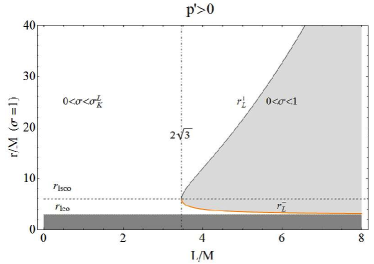
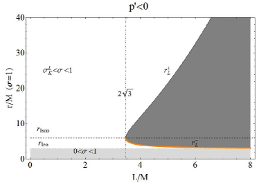
Figure 26: (Color online) Left panel: conditions for $G_{r}>0$: $0\leq\sigma<\sigma_{\mbox{\tiny{K}}}^{\mbox{\tiny{L}}}$ when $0<L<2\sqrt{3}M$ and $r>r_{lco}$, and when $L>2\sqrt{3}M$ and $r_{lco}<r<r_{\mbox{\tiny{L}}}^{-}(\sigma=1)$ and $r>r_{\mbox{\tiny{L}}}^{+}(\sigma=1)$. $G_{r}>0$ for all $0<\sigma<1$ when $L>2\sqrt{3}M$ and $r_{\mbox{\tiny{L}}}^{-}(\sigma=1)<r<r_{\mbox{\tiny{L}}}^{+}(\sigma=1)$, while it is always positive when $r<r_{lco}$. Right panel: conditions for $G_{r}<0$: $\sigma_{\mbox{\tiny{K}}}^{\mbox{\tiny{L}}}<\sigma<1$ when $0<L<2\sqrt{3}M$ and $r>r_{lco}$, and when $L>2\sqrt{3}M$ and $r_{lco}<r<r_{\mbox{\tiny{L}}}^{-}(\sigma=1)$ and $r>r_{\mbox{\tiny{L}}}^{+}(\sigma=1)$. $G_{r}<0$ for all $0<\sigma<1$ when $r<r_{lco}$, while it is always negative when $L>2\sqrt{3}M$ and $r_{\mbox{\tiny{L}}}^{-}(\sigma=1)<r<r_{\mbox{\tiny{L}}}^{+}(\sigma=1)$. Dotted lines mark $r=r_{lco}$, dashed lines $r=r_{lsco}$, dot-dashed lines $L=2\sqrt{3}M$.

We characterize now the angular momentum $L$ as an explicit function of $l$ and $\sigma$. We know from Section 3.2 that $L$ is not defined in the interval $[r^{-}_{l},r^{+}_{l}]$, where $r_{l}^{\pm}$ are introduced in Eq. 19. In terms of $\sigma$ this region corresponds to $0\leq a\leq\sigma_{l_{r}}$, where $\sigma_{l_{r}}\equiv\sqrt{\frac{l^{2}(r-2M)}{r^{3}}}$. $\sigma_{l_{r}}$ is defined for $r>2M$ when $0<l\leq 3\sqrt{3}M$, and for $2M<r<r_{l}^{-}(\sigma=1)$ and $r>r_{l}^{+}(\sigma=1)$ when $l>3\sqrt{3}M$. $r=r_{lco}$ is a maximum for $\sigma_{l_{r}}$, where $\sigma_{l_{r}}=\sigma_{l_{r}}^{*}\equiv\frac{\sqrt{l^{2}}}{3\sqrt{3}M}$. When $l=3\sqrt{3}M$, it is $\sigma_{l_{r}}^{*}=1$.

Table 1: Regions where $\partial_{r}L=0$.

$0<l/M\leq 3\sqrt{3/2}$		$3\sqrt{3/2}<l/M<3\sqrt{3}$		$l/M\geq 3\sqrt{3}$
$\sigma$	$r/M$	$\sigma$	$r/M$	$\sigma$	$r/M$
$(0,\sigma_{l_{r}}^{*}]$	$r_{+}$	$(0,\sigma_{l_{r}}^{*}]$	$r_{+}$	$(0,1]$	$r_{+}$
$(\sigma_{l_{r}}^{*},\sqrt{2}\sigma_{l_{r}}^{*})$	$r_{+}$, $r_{-}$	$(\sigma_{l_{r}}^{*},1]$	$r_{+}$, $r_{-}$
$\sqrt{2}\sigma_{l_{r}}^{*}$	$r_{+}=r_{-}=r_{lsco}$

The critical points of $L$ are determined by the condition:

$$\sigma_{\mbox{\tiny{K}}}^{\mbox{\tiny{l}}}\equiv\sqrt{\frac{l^{2}(r-2M)^{2}}{Mr^{3}}}\,.$$ (114)

(see Eq. 20). $\sigma_{\mbox{\tiny{K}}}^{\mbox{\tiny{l}}}$ is defined for $r>r_{lco}$ when $0<l\leq 3\sqrt{3/2}M$, and for $r_{lco}<r\leq r_{-}(\sigma=1)$ and $r\geq r_{+}(\sigma=1)$ when $3\sqrt{3/2}M<l<3\sqrt{3}M$, and also for $r\geq r_{+}(\sigma=1)$ for $l\geq 3\sqrt{3}M$, where $r_{\pm}(\sigma=1)$ are the radii defined by Eq. 21, evaluated at $\sigma=1$. $\sigma_{\mbox{\tiny{K}}}^{\mbox{\tiny{l}}}$ is maximum for $r=r_{lsco}$, where $\sigma_{\mbox{\tiny{K}}}^{\mbox{\tiny{l}}}=\sigma_{\mbox{\tiny{K}}}^{\mbox{\tiny{l}}*}=\sqrt{2}\sigma_{l_{r}}^{*}$. These results are summarized in Table 1.

Finally the study of $G_{r}$ as a function of $(r,l,\sigma)$ is illustrated in Figs. 27.

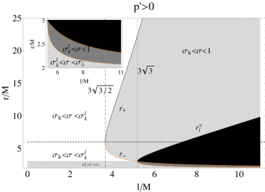
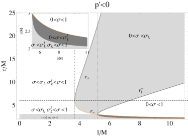
Figure 27: (Color online) Left panel: conditions for $G_{r}>0$: $\sigma_{l_{r}}<\sigma<\sigma_{\mbox{\tiny{K}}}^{\mbox{\tiny{l}}}$ when $0<l<3\sqrt{3/2}M$ and $r>r_{lco}$, and when $3\sqrt{3/2}M<l<3\sqrt{3}M$ and $r_{lco}<r<r_{-}(\sigma=1)$ and $r>r_{+}(\sigma=1)$, and when $l>3\sqrt{3}M$ and $r>r_{+}(\sigma=1)$; $\sigma_{l_{r}}<\sigma<1$ when $3\sqrt{3/2}M<l<3\sqrt{3}M$ and $r_{-}(\sigma=1)<r<_{+}(\sigma=1)$, and when $l>3\sqrt{3}M$ and $r_{l}^{+}(\sigma=1)<r<r_{+}(\sigma=1)$; $\sigma_{\mbox{\tiny{K}}}^{\mbox{\tiny{l}}}<\sigma<1$ when $l>3\sqrt{3}M$ and $r_{l}^{-}(\sigma=1)<r<r_{-}(\sigma=1)$; $\sigma_{\mbox{\tiny{K}}}^{\mbox{\tiny{l}}}<\sigma<\sigma_{l_{r}}$ when $l<3\sqrt{3}M$ and $2M<r<r_{lco}$, and when $l>3\sqrt{3}M$ and $2M<r<r_{l}^{-}(\sigma=1)$. Right panel: conditions for $G_{r}>0$: $0<\sigma<\sigma_{l_{r}}$ and $\sigma_{\mbox{\tiny{K}}}^{\mbox{\tiny{l}}}<\sigma<1$ when $0<l<3\sqrt{3/2}M$ and $r>r_{lco}$, and when $3\sqrt{3/2}M<l<3\sqrt{3}M$ and $r_{lco}<r<r_{-}(\sigma=1)$ and $r>r_{+}(\sigma=1)$, and when $l>3\sqrt{3}M$ and $r>r_{+}(\sigma=1)$; $)<\sigma<\sigma_{l_{r}}$ when $3\sqrt{3/2}M<l<3\sqrt{3}M$ and $r_{-}(\sigma=1)<r<_{+}(\sigma=1)$, and when $l>3\sqrt{3}M$ and $r_{l}^{+}(\sigma=1)<r<r_{+}(\sigma=1)$; $0<\sigma<\sigma_{\mbox{\tiny{K}}}^{\mbox{\tiny{l}}}$ when $l>3\sqrt{3}M$ and $r_{l}^{-}(\sigma=1)<r<r_{-}(\sigma=1)$; $0<\sigma<\sigma_{\mbox{\tiny{K}}}^{\mbox{\tiny{l}}}$ and $\sigma_{l_{r}}<\sigma<1$ when $l<3\sqrt{3}M$ and $2M<r<r_{lco}$, and when $l>3\sqrt{3}M$ and $2M<r<r_{l}^{-}(\sigma=1)$. $G_{r}<0$ for all $0<\sigma<1$ when $L>3\sqrt{3}M$ and $r_{-}(\sigma=1)<r<r_{l}^{+}(\sigma=1)$. Dotted lines mark $l=3\sqrt{3}M$, dot-dashed lines $l=3\sqrt{3/2}M$, dashed lines $r=r_{lsco}$ and dotted gray lines $r=r_{lco}$. Black regions are forbidden. Insets: zoom of the region $l/M\in[6,11]$ and $r/M\in[2,r_{lco}]$.

Appendix B Analysis of the proper velocity profile

We redefine the radius in Eq. 97 in terms of $\sigma$ and $l$:

$$r_{\chi}/M=\frac{1}{4}\left(\frac{5}{2}-\frac{\beta}{2\sqrt{3}}+\frac{\check{\beta}}{\sqrt{6}}\right)\,,$$ (115)

where

$$\check{\beta} \equiv \sqrt{\frac{264\sqrt{3}(l/M)^{2}\alpha-4\left[(l/M)^{4}-4(l/M)^{2}\alpha+\alpha^{2}\right]\beta+\sigma^{2}\left[144(l/M)^{2}\beta+75\alpha\left(\beta-5\sqrt{3}\right)\right]}{\sigma^{2}\alpha\beta}},$$ (116)

$$\alpha \equiv \left[-(l/M)^{2}\left(1350\sigma^{4}+(l/M)^{4}-6\sigma^{2}\left[9(l/M)^{2}+\sqrt{48(l/M)^{4}-2754\sigma^{2}(l/M)^{2}+50625\sigma^{4}}\right]\right)\right]^{1/3},$$ (117)

$$\beta \equiv \sqrt{\frac{8\left[(l/M)^{2}+\alpha\right]^{2}+\sigma^{2}\left[75\alpha-288(l/M)^{2}\right]}{\sigma^{2}\alpha}},$$ (118)

for $\sigma\neq 0$ (for $\sigma=0$ it is $r^{\pm}_{\chi}=2M$).

The fluid proper angular velocity increases with $r/M$ ($\Phi^{\prime}>0$) when:

$$0<l<3\sqrt{3}M\quad\mbox{for}\quad 0<\sigma\leq\sigma_{l_{r}}\quad\mbox{and}\quad 2M<r<r_{l}^{-}\,,$$ (119)

$$\sigma_{l_{r}}<\sigma\leq 1\quad\mbox{and}\quad 2M<r<r_{\chi}\,;$$ (120)

$$l\geq 3\sqrt{3}M\quad\mbox{for}\quad 0<\sigma\leq 1\quad\mbox{and}\quad 2M<r<r_{l}^{-}\,.$$ (121)

It is $\Phi^{\prime}<0$ when:

$$0<l<3\sqrt{3}M\quad\mbox{for}\quad 0<\sigma<\sigma_{l_{r}}\quad\mbox{and}\quad r>r_{l}^{+}\,,$$ (122)

$$\sigma=\sigma_{l_{r}}\quad\mbox{and}\quad r>r_{l}^{-}\,,$$ (123)

$$\sigma_{l_{r}}<\sigma\leq 1\quad\mbox{and}\quad r>r_{\chi}\,;$$ (124)

$$l=3\sqrt{3}M\quad\mbox{for}\quad 0<\sigma<1\quad\mbox{and}\quad r>r_{l}^{+}\,,$$ (125)

$$\sigma=1\quad\mbox{and}\quad r>r_{l}^{-}\,;$$ (126)

$$l>3\sqrt{3}M\quad\mbox{for}\quad 0<\sigma\leq 1\quad\mbox{and}\quad r>r_{l}^{+}$$ (127)

(see Fig. 28). It follows that the angular velocity increases in $2M<r<r_{\chi}<3M$ until it reaches the point $r=r_{\chi}$, that is a maximum, where $2.5M<r_{\chi}<3M$ with angular momentum $l_{\chi}$ on the equatorial plane $\sigma_{\chi}$, then it decreases with the radius (see Fig. 28).

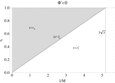
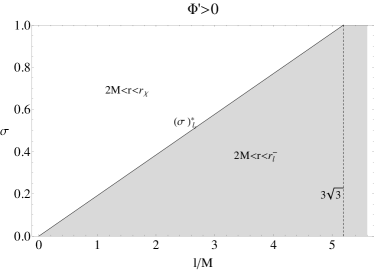
Figure 28: Left panel: conditions for $\Phi^{\prime}<0$. Right panel: conditions for $\Phi^{\prime}>0$. Solid line marks $\sigma_{l_{r}}^{*}$ as a function of $l/M$, dashed line $l/M=3\sqrt{3}$.

References

- (1) Abramowicz M. A., 1971, Acta Astron., 21, 81
- (2) Abramowicz M. A., 1981, Nat. 294, 235
- (3) Abramowicz M. A., 2005, in Merloni A., Nayakshin S., Sunyaev R., eds, ESO Astrophysics Symposia, Growing Black Holes: Accretion in a Cosmological Context. Springer-Verlag, Berlin, p. 257
- (4) Abramowicz M. A., 2008, preprint (astro-ph/0812.3924)
- (5) Abramowicz M. A., 2009, A&A, 500, 213
- (6) Abramowicz M. A., Fragile P. C., 2011, preprint (astro-ph/1104.5499 )
- (7) Abramowicz M. A., Jaroszyński M., Sikora M., 1978, A&A, 63, 221
- (8) Abramowicz M. A., Calvani M., Nobili L., 1980, ApJ, 242, 772
- (9) Abramowicz M. A., Lanza A., Percival M. J., 1997, ApJ, 479, 179
- (10) Abramowicz M. A., Karas V., Lanza A., 1998, A&A, 331, 1143
- (11) Balbus S.A., 2011, Nat., 470, 475
- (12) Blaes O.M., 1987, MNRAS, 227, 975.
- (13) Boyer R. H., 1965, MPCPS, 61, 527
- (14) Chakrabarti S. K., 1990, MNRAS, 245, 747
- (15) Chakrabarti S. K., 1991, MNRAS, 250, 7
- (16) De Villiers J-P, Hawley J. F., 2002, ApJ, 577, 866
- (17) Fender R., Belloni T., 2004, Ann. Rev. Astron. Astrophys., 42, 317
- (18) Fishbone L. G., Moncrief V., 1976, ApJ, 207, 962
- (19) Font J. A., 2003, Living Rev. Relat., 6, 4
- (20) Fragile P. C., Blaes O. M., Anninois P., Salmonson J. D., 2007, preprint (astro-ph/0706.4303)
- (21) Frank J., King A., Raine D., 2002, Accretion Power in Astrophysics, Cambridge University Press, Cambridge
- (22) Horedt G. P. 2004, Polytropes: Applications in Astrophysics and Related Fields, Klawer Academic Publishers, Dordrecht
- (23) Hawley J. F., 1987, MNRAS, 225, 677
- (24) Hawley J. F., 1990, ApJ,356, 580
- (25) Hawley J. F., 1991, ApJ, 381, 496
- (26) Hawley J. F., Smarr L. L., Wilson J. R., 1984, ApJ, 277, 296
- (27) Igumenshchev I.V., Abramowicz M. A., 2000, ApJS, 130, 463
- (28) Jaroszynski M., Abramowicz M. A., Paczynski B., 1980, Acta Astronm., 30, 1
- (29) Kozłowski M., Jaroszyński M., Abramowicz M. A., 1978, A&A, 63, 209
- (30) Kucakova H., Slany P., Stuchlik Z., 2011, JCAP, 01, 033
- (31) Lei Q., Abramowicz M. A., Fragile P. C., Horak J., Machida M., Straub O., 2009, A&A, 498, 471
- (32) Misner C. W., Thorne K. S., Wheeler J. A., 1973, Gravitation, Freeman, San Francisco
- (33) Paczyński B., 1980, Acta Astron., 30, 4
- (34) Paczyński B., Wiita P., 1980, A&A, 88, 23
- (35) Pugliese D., Quevedo H., Ruffini R., 2011a, Phys. Rev. D, 84, 044030
- (36) Pugliese D., Quevedo H., Ruffini R., 2011b, Phys. Rev. D, 83, 104052
- (37) Pugliese D., Quevedo H., Ruffini R., 2011c, Phys. Rev. D, 83, 024021
- (38) Rezzolla L., Zanotti O., Font J. A., 2003, A&A, 412, 603
- (39) Seguin F. H., 1975, ApJ, 197, 745
- (40) Shakura N.I., Sunyaev R.A., 1973, A&A, 24, 337-355
- (41) Shafee R., McKinney J.C., Narayan R., Tchekhovosky A., Gammie C.F, McClintock J.E., 2008, ApJ, 687, L25
- (42) Slaný P., Stuchlík Z., 2005, Class. Quantum Gravity, 22, 3623
- (43) Soria R., 2007, Astrophysics and Space Science, 311, 213
- (44) Straub O.,Vincent F. H., Abramowicz M. A., Gourgoulhon E. and Paumard T., 2012, preprint (astro-ph/1203.2618)
- (45) Stuchlík Z., 2000, Acta Phys. Slovaca, 50, 219
- (46) Stuchlík Z., Kovář J., 2008, Int. J. Mod Phys D, 17
- (47) Stuchlík Z., Slaný P., 2006, AIP Conf. Proc. 861, 770
- (48) Stuchlík Z., Slaný P., Hledík S, 2000, A&A, 363, 425
- (49) Stuchlík Z., Slaný P., Kovar J., 2009, Class. Quantum Gravity, 26, 215013
- (50) Tsagas C. G., 2005, Class. Quantum Gravity, 22, 393
- (51) Wald R. M., 1984, General Relativity, University of Chicago Press, Chicago