Evaluating Overlapping Communities
with the Conductance of their Boundary Nodes

Abstract

Usually the boundary of a community in a network is drawn between nodes and thus crosses its outgoing links. If we construct overlapping communities by applying the link-clustering approach nodes and links interchange their roles. Therefore, boundaries must drawn through the nodes shared by two or more communities. For the purpose of community evaluation we define a conductance of boundary nodes of overlapping communities analogously to the graph conductance of boundary-crossing links used to partition a graph into disjoint communities. We show that conductance of boundary nodes (or normalised node cut) can be deduced from ordinary graph conductance of disjoint clusters in the network’s weighted line graph introduced by evans2009line to get overlapping communities of nodes in the original network. We test whether our definition can be used to construct meaningful overlapping communities with a local greedy algorithm of link clustering. In this note we present encouraging results we obtained for Zachary’s karate-club network.

1 Introduction

A community in a network is usually defined as a subgraph that is both cohesive and well separated from the rest of the network [FortunatoFortunato2010]. Cohesion and separation can be evaluated by various measures. A simple absolute measure of cohesion is the sum of weights of links between all members $C$ of a subgraph which equals their total internal degree $k_{\mathrm{in}}(C)$ divided by 2. A simple absolute measure of separation is the sum of weights of links between members and non-members which equals the total external degree $k_{\mathrm{out}}(C)$. A single function sensitive to a subgraph’s cohesion and separation is the normalised cut

$$\Phi(C)=\frac{k_{\mathrm{out}}(C)}{k_{\mathrm{in}}(C)+k_{\mathrm{out}}(C)}.$$

The total external degree $k_{\mathrm{out}}(C)$ equals the total electrical conductance of the links cut by $C$’s boundary if each link’s conductance is defined by its weight. Therefore $\Phi(C)$ is also named conductance. If the cut through external links of a subgraph with node set $C$ has minimal conductance $\Phi(C)$ then $C$ can be called a community. yang2012defining tested 13 evaluation functions and found that evaluating subgraphs with conductance $\Phi$ results in good disjoint communities.

These ideas can also be applied when the perspective on the network is changed and communities of links instead of communities of nodes are to be constructed. This approach was introduced by evans2009line and by ahn2010link with the aim to obtain overlapping node communities. The definition of a community as a cohesive and separated subgraph still holds for this perspective. The important difference between communities of nodes and communities of links is that the latter’s boundaries cuts through nodes instead of links. When community boundaries shift from links to nodes, the evaluation function needs to be changed accordingly. In this paper, we introduce the normalised node cut $\Psi$ as an evaluation function for link communities.

evans2009line found that a network’s line graph can be used to obtain link communities. They applied modularity—a global evaluation function—to obtain link communities but stressed that any method for community construction can be applied to the line graph. We show that evaluating a network’s subgraphs with the normalised node cut $\Psi$ is equivalent to an evaluation of subgraphs in the network’s line graph with ordinary normalised edge cut $\Phi$ if each edge in the line graph is weighted with the degree of the corresponding node as proposed by evans2009line.

We test whether the normalised node cut $\Psi$ can be used to evaluate subgraphs and thus to find a network’s link communities. For this purpose we construct a $\Psi$-landscape. A community of links is defined as a subgraph with a local $\Psi$-minimum. We apply a greedy local expansion algorithm to find local minima in the $\Psi$-landscape. We present results obtained for a simple benchmark, the karate-club network analysed by zachary1977information.

2 Method

2.1 Normalised Node Cut

Since the boundary of a link community consists of nodes, the measure of cohesion and separation must be shifted accordingly. We define the normalised node cut $\Psi(C)$ of a connected subgraph with node set $C$ as the normalised total conductance of $C$’s boundary nodes given by

$$\begin{split}\Psi(C)&=\frac{1}{k_{\mathrm{in}}(C)}\sum_{i\in C}\frac{1}{1/k_{i}^{\mathrm{in}}(C)+1/k_{i}^{\mathrm{out}}(C)}\\ &=\frac{1}{k_{\mathrm{in}}(C)}\sum_{i\in C}\frac{k_{i}^{\mathrm{in}}(C)k_{i}^{\mathrm{out}}(C)}{k_{i}}.\end{split}$$ (1)

Here $k_{i}^{\mathrm{in}}(C)$ is the internal degree of node $i$, i.e. the total weight of its links to other $C$-members, and $k_{i}^{\mathrm{out}}(C)$ its external degree, i.e. the total weight of its links to non-members. Both sum up to the total degree of node $i$, which does not depend on $C$: $k_{i}=k_{i}^{\mathrm{in}}(C)+k_{i}^{\mathrm{out}}(C)$.

Each term in the sum of equation 1 equals the electrical conductance between external and internal nodes connected through node $i$ if we identify the link weights with electrical conductances. Since the external degree $k_{i}^{\mathrm{out}}(C)$ of inner nodes is zero, the sum includes only the nodes that constitute $C$’s boundary.

The normalised node cut $\Psi$ is defined for weighted networks. For the sake of simplicity, we restrict the discussion to unweighted networks in the remainder of the paper. In this case, $k_{i}^{\mathrm{in}}(C)$ equals the number of links between node $i$ and other members of $C$ and $k_{i}^{\mathrm{out}}(C)$ is the number of links between $i$ and nodes outside $C$.

For the complete graph, which has no outgoing links, $\Psi=0$ because for all nodes $k_{i}^{\mathrm{out}}=0$. Furthermore, the normalisation in equation 1 guarantees that $\Psi<1$ for all subgraphs because $\Psi$ equals the $k_{i}^{\mathrm{in}}$-weighted average of relative external degrees $k_{i}^{\mathrm{out}}/k_{i}<1$.

Function $\Psi(C)$ decreases with increasing internal cohesion (measured by $k_{\mathrm{in}}(C)$) and with decreasing linkage with the rest of the network (measured with the sum in equation 1). Thus, $\Psi(C)$ is a function sensitive to a subgraph’s cohesion and separation.

Our definition of the normalised node cut $\Psi$ can be derived by applying the normalised edge cut $\Phi$ in the network’s line graph with weights $1/k_{i}$. This weighting was proposed by evans2009line. To construct a network’s line graph we first define an auxiliary bipartite graph obtained by putting a node on each link of the original network. The affiliation matrix $B$ of the bipartite graph—also called its incidence matrix—has a row for each of the $n$ original nodes and a column for each of the $m$ original links. Each link column contains only two non-zero elements, namely the elements in the rows of the nodes $i$ and $j$ connected by the link. We can project the bipartite graph back onto the original network with the product $BB^{\mathrm{T}}$ which equals its adjacency matrix $A$ (except for the main diagonal).

We obtain the network’s line graph by the opposite projection $B^{\mathrm{T}}B$ of the bipartite graph. evans2009line emphasise, that the line graph contains the same amount of information as the original network in all cases of practical interest. Knowing $B^{\mathrm{T}}B$ we can almost always calculate $BB^{\mathrm{T}}$ and thus also the network’s adjacency matrix $A$.

evans2009line weight the edges of the line graph with the inverse degree $1/k_{i}$ of the node $i$ in the original network because each node is represented as a clique in the line graph. They define the line graph’s adjacency matrix as

$$E_{kl}=\sum_{i=1}^{n}\frac{B_{ik}B_{il}}{k_{i}}.$$ (2)

For this line graph we can calculate the ordinary graph conductance or normalised cut $\Phi$ of a link set $L$ and get $\Phi(L)=\Psi(C(L))$, where $C(L)$ is the set of nodes attached to links in $L$. The proof can be found in the appendix (p. Acknowledgements).

Different link sets $L$ can have the same induced node set $C(L)$ if we define $C(L)$ to be the set of all nodes attached to links in $L$. We define the link set $L(C)$ induced by $C$ as the maximum set of links (existing in the network) that induces $C$. A connected subgraph’s link set is assumed to be a maximum set. It is induced by the subgraph’s node set. If we would not include all existing links between all nodes of a subgraph in its link set we would have external links between member nodes. We could even change two adjacent inner nodes to boundary nodes if we would omit the link connecting them from the subgraph’s link set.

Weighting the line graph’s edges with the inverse degrees of nodes in the original network is equivalent to an Euclidean normalisation of the nodes’ vectors in the affiliation matrix $B$ of the auxiliary bipartite graph. This becomes clear if we factorise the terms of the sum in equation 2:

$$E_{kl}=\sum_{i=1}^{n}\frac{B_{ik}}{\sqrt{k_{i}}}\frac{B_{il}}{\sqrt{k_{i}}}.$$ (3)

Then we can shortly write $E=D^{\mathrm{T}}D$ with $D_{ik}=B_{ik}/\sqrt{k_{i}}$ and verify the Euclidean normalisation of the $n$ row vectors of $D$:

$$\sum_{k=1}^{m}D_{ik}^{2}=\sum_{k=1}^{m}\frac{B_{ik}^{2}}{k_{i}}=\frac{1}{k_{i}}\sum_{k=1}^{m}B_{ik}=1.$$ (4)

Here we used that $B$ is binary (because $A$ is binary for unweighted networks) and therefore $B_{ik}^{2}=B_{ik}$.

The projection of the normalised bipartite graph described by affiliation matrix $D$ back on a network of the original nodes is given by $DD^{\mathrm{T}}$. Any element of adjacency matrix $DD^{\mathrm{T}}$ (except for the main diagonal) is given by

$$\sum_{k=1}^{m}D_{ik}D_{jk}=\sum_{k=1}^{m}\frac{B_{ik}B_{jk}}{\sqrt{k_{i}k_{j}}}=\frac{A_{ij}}{\sqrt{k_{i}k_{j}}}.$$ (5)

This means that the Euclidean normalisation of $B$’s row vectors is equivalent to weighting each link in the original (unweighted) network with the geometric mean of its nodes’ inverse degrees. The weighted graph described by adjacency matrix $E$ is not the line graph of the unweighted network described by adjacency matrix $A$ but the line graph of the network weighted according to equation 5. The approach is applicable only to those networks for which the weighting with the geometric means is a realistic assumption.

2.2 Defining Communities

Local greedy algorithms construct communities by starting from seeds and adding those neighbours of the subgraph which maximally improve or minimally downgrade its cohesion and separation. Due to its locality, this approach can be used to construct a seed’s nested sequence of communities in a network which is too large to process it totally [ClausetClauset2005, Luo, Wang, and PromislowLuo et al.2008, Havemann, Heinz, Struck, and GläserHavemann et al.2011]. In the case of link communities, the local greedy expansion of subgraphs should start from links as seeds and iteratively add new links.

We construct a landscape of the normalised node cut $\Psi(C)$ of connected subgraphs. Each connected subgraph consists of a node set $C$ and the link set $L(C)$ containing all links that exist between nodes in $C$. Each place in the landscape represents a connected subgraph defined by its node set $C$. A relation between two places exists if one of the subgraphs can be obtained by adding a node to the other one. The height of a place is the subgraph’s $\Psi$-value. Communities can be defined as those subgraphs whose $\Psi$-values are local minima in the $\Psi$-landscape.

Any two places in the $\Psi$-landscape are connected by paths. To reach one place from another one we have to add and remove nodes of the corresponding subgraphs. The absolute distance between two places in the $\Psi$-landscape is the number of steps one has to go on a shortest path between them. These are $|M\cup N|-|M\cap N|$ steps, where $M$ and $N$ are the node sets of the two connected subgraphs. We obtain the Jaccard distance by normalising the absolute distance with $|M\cup N|$.

The distance between two communities can be used to define a community’s stability. A community’s stability is the shortest Jaccard distance to a community with a lower $\Psi$-value. A community is more cohesive and better separated from the rest of the network than all other communities within the radius of the shortest Jaccard distance to a community with a lower $\Psi$-value.

The communities evaluated by $\Psi$ are connected subgraphs that grow by adding neighbouring nodes with all their links to the community. However, it is justified to treat these communities as link communities because the community’s boundary consists of nodes. Expanding a link community means shifting its boundary from one set of nodes to another, while the node communities commonly discussed in the literature are expanded by shifting their boundaries from one set of links to another.

2.3 Identifying Communities
with a Greedy Algorithm

Constructing the whole $\Psi$-landscape is not feasible for larger networks. However, algorithms for the search of stable local minima in the $\Psi$-landscape can be constructed. We tested a greedy algorithm that adds those nodes that incur either the greatest reduction in $\Psi$ (i.e. go down the steepest slope in the $\Psi$-landscape) or the smallest increase in $\Psi$ (i.e. go up the gentlest slope in the $\Psi$-landscape).

Starting from a seed link, we go downhill in the $\Psi$-landscape on the path with the steepest slope. This slope is produced by adding to the subgraph the neighbouring node that incurs the greatest reduction in $\Psi$. If the $\Psi$-balance of two candidate nodes is tied we randomly select a path. Experiments showed that in most cases the two paths created by nodes with tied $\Psi$-balance will merge soon. If adding any neighbouring node to a subgraph increases $\Psi$, we search for members of the subgraph whose exclusion further reduces $\Psi$. If we don’t find such members then we have reached a local $\Psi$-minimum. If we do, we prune the subgraph by excluding them and try again to add a neighbour which maximally reduces $\Psi$. If this trial fails then we have also reached a minimum.

After a local minimum has been reached, we continue to add nodes. Initially, nodes producing the smallest increase in $\Psi$ must be added for the algorithm to leave the hollow in the $\Psi$-landscape created by the local minimum. Thereafter, the search for the steepest slope can be resumed. This is repeated until we reach the ground state of the whole (connected) network with $\Psi=0$. If all links of a network are used as seeds, there is a high likelihood that all local minima are found or at least all those with high stability.

For larger networks it takes much time to determine the path for each link. It is possible to save computing time by an updating of node sets and variables needed for the iterative procedure. In appendix A.2 we describe how the sum in the $\Psi$-function can be updated during the iteration.

3 Experiments

3.1 Karate Club

The club of 34 karate fighters observed by zachary1977information split up into two disjoint parts of equal size. The links between the fighters were weighted with their interactions at different places. The network of the karate club became a benchmark graph that is often used for testing cluster algorithms, including algorithms for the construction of overlapping communities. In our experiments, we used the unweighted version of the network.

We applied the greedy algorithm described above to each of the 78 links of the network. The algorithm found seven local minima in the network’s $\Psi$-landscape. Table 1 lists for each minimum the number of links, the number of nodes, the normalised node cut $\Psi$, and the number of seed links from which the minimum has been found.

Table 1: Communities found in the karate network

name	links	nodes	$\Psi$	seeds
$C_{1}$	68	29	.022	68
$C_{2}$	43	21	.077	40
$C_{3}$	41	19	.091	10
$C_{4}$	10	6	.150	10
$C_{5}$	6	5	.294	7
$C_{6}$	2	3	.460	2
$C_{7}$	1	2	.469	1

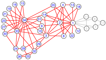
Figure 1: Community $C_{1}$ has 29 nodes (blue) and 68 links (red). The ten grey links of community $C_{4}$ connect six nodes including the boundary node 1.

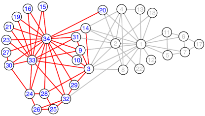
Figure 2: Community $C_{2}$ has 21 nodes (blue) and 43 links (red). Community $C_{3}$ has 19 nodes (connected by grey links). Both communities share six boundary nodes (connecting grey and red links).

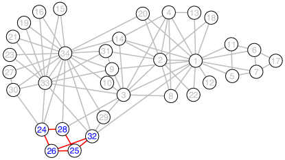
Figure 3: Community $C_{5}$ has five nodes (blue) and six links (red).

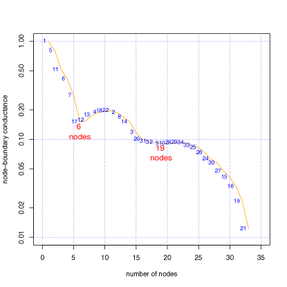
Figure 4: $\Psi$-plot of seed link (1, 5) with minima of communities $C_{4}$ and $C_{3}$

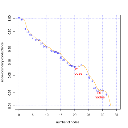
Figure 5: $\Psi$-plot of seed link (33, 34) with minima of communities $C_{2}$ and $C_{1}$

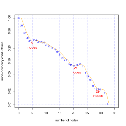
Figure 6: $\Psi$-plot of seed link (25, 26) with minima of communities $C_{5}$, $C_{2}$, and $C_{1}$

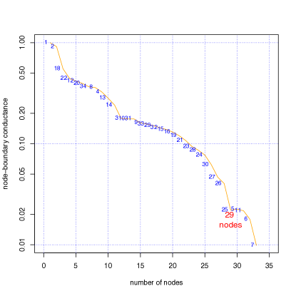
Figure 7: $\Psi$-plot of seed link (1, 2) with minimum of community $C_{1}$

The largest community $C_{1}$ with 29 nodes has only one boundary node, namely node 1 (s. Fig. 1). The same one-node boundary delineates community $C_{4}$ with six nodes. The union of $C_{1}$ and $C_{4}$ covers the whole network, their intersection contains only node 1. Analogously, the union of $C_{2}$ and $C_{3}$ also covers the network. Their intersection contains their common boundary nodes, namely nodes 3, 9, 14, 20, 31, and 32 (s. Fig. 2). The other three communities are subsets of larger communities, $C_{5}$ and $C_{6}$ of $C_{2}$, and $C_{7}$ of $C_{1}$ and $C_{3}$. Community $C_{5}$ has five nodes as members (s. Fig. 3), $C_{6}$ only three (nodes 3, 10, and 34). Community $C_{7}$ is the pair of nodes 1 and 12.

At least one local minimum of $\Psi$ was found in each run. 27 of the 78 seed links led to one local minimum, 42 to two local minima, and nine to three local minima. All ten links of community $C_{4}$ led to $C_{3}$ and $C_{4}$. As an example of the paths through the $\Psi$-landscape, Fig. 4 shows the plot of $\Psi$ over the number of nodes obtained by starting from seed link $(1,5)$. Since the $\Psi$-scale in Fig. 4 is logarithmic, the last point of the $\Psi$-curve, which represents the whole network with $\Psi=0$, is not visible.

40 of 43 links of $C_{2}$ found $C_{1}$ and $C_{2}$. As an example, we show the $\Psi$-plot of seed link (33, 34) in Fig. 5. The two links of $C_{6}\subset C_{2}$ found also $C_{6}$, the six links of $C_{5}\subset C_{2}$ also $C_{5}$. In Fig. 6 we plot $\Psi$ of seed (25, 26).

Community $C_{6}$ is also present as a local minimum when we start from seed (3, 28). However, in this case node 3 is excluded in the pruning process because excluding it further reduces $\Psi$. Community $C_{7}$ is identical to its seed link (1, 12). All other 27 links led the algorithm to only one local minimum, namely that of $C_{1}$. All these links belong to $C_{3}$. As a further example, we plot the $\Psi$-curve of seed (1, 2) in Fig. 7.

Two pairs of communities found by the greedy algorithm each cover the whole network and overlap in their boundary nodes, namely the pair $C_{2}$ and $C_{3}$ and the pair $C_{1}$ and $C_{4}$. The cut by the boundary nodes between $C_{2}$ and $C_{3}$ is compatible with the final split of the karate club and corresponds to one solutions found by evans2009line. Four of the six fighters on the boundary between $C_{2}$ and $C_{3}$ (nodes 3, 9, 14, 20) decided to follow Mr. Hi (node 1) and the other two (nodes 31 and 32) joined the officer’s club (node 34).

Note that not only $C_{2}$ and $C_{3}$ overlap but also their link sets $L(C_{2})$ and $L(C_{3})$: $L(C_{2})\cap L(C_{3})=\{(3,9),(9,31)\}.$ This is a special feature of our greedy algorithm based on the normalised node cut. The link clustering procedures proposed by ahn2010link and by evans2009line produce only disjoint link clusters.

In our example, two nested tree-like hierarchies of communities can be observed:

1. the whole graph splits into $C_{1}$ and $C_{4}$ which overlap in boundary node 1, and $C_{1}$ has several communities as subgraphs:

   1. $C_{2}$ with $C_{5}$ and $C_{6}$ as subgraphs,

   2. $C_{7}$,

2. the whole graph splits into $C_{2}$ and $C_{3}$ which overlap in six boundary nodes, and each has two communities as subgraphs:

   1. $C_{2}$ contains $C_{5}$ and $C_{6}$,

   2. $C_{3}$ contains $C_{4}$ and $C_{7}$.

$C_{3}$ is missing in the first hierarchy and $C_{1}$ in the second. These two communities cannot appear in the same nested tree-like hierarchy because they have a permeating overlap, i.e. they share not only boundary nodes but also inner nodes. The occurrence of such permeating overlaps is also a new feature of our approach which is absent in the approaches proposed by ahn2010link and by evans2009line. If permeating overlap is a realistic assumption we obtain one solution for the karate-graph but this solution is a polyhierarchy rather than a tree-like hierarchy because $C_{7}$ is a subgraph of both $C_{1}$ and $C_{3}$ (s. Fig. 8). In most cases, combined sub-communities do not completely cover the higher-level communities they are part of. The only exception is the whole graph $C_{0}$, which is completely covered by the pair $(C_{1},C_{4})$ and also by the pair $(C_{2},C_{3})$.

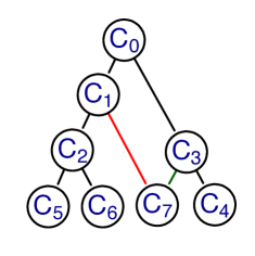
Figure 8: Polyhierarchy of all link communities of the karate-club network (symbolised by $C_{0}$). Lower-level communities are subgraphs of higher-level ones. When $C_{1}$ and the red or $C_{3}$ and the green link are omitted we obtain one of the two alternative tree-like hierarchies (s. text).

4 Summary and Conclusions

We propose to see a community being connected via nodes and not via links to the rest of the network. These boundary nodes can be shared by two or more communities. To evaluate overlapping communities we define a normalised node cut $\Psi$ analogously to usual normalised cut $\Phi$ used to construct disjoint communities. We define a community $C$ as a connected subgraph corresponding to a local minimum in a $\Psi$-landscape over all connected subgraphs which are linked by inclusion of a subgraph’s neighbour or exclusion of a member. Applying a greedy algorithm, we found seven local $\Psi$-minima of the karate-club network from which nested hierarchies of overlapping communities can be constructed. One pair of communities overlapping in their boundary nodes is compatible with the final split of the karate club. Further tests on benchmark graphs are in preparation.

Normalised node cut $\Psi$ only uses degrees of nodes as input and can therefore be calculated also for weighted graphs. A greedy algorithm may not find all local minima in the $\Psi$-landscape of connected subgraphs. Whether local $\Psi$-minima represent useful communities depends on the part of reality we model with our network.

Appendix A Appendix

A.1 Proof of $\Psi(C)=\Phi(L)$

Normalised node cut $\Psi(C)$ of a subgraph in a network equals normalised edge cut $\Phi(L)$ of the corresponding subgraph in the network’s line graph weighted according to evans2009line, as we will show now.

Like in equation 2 we here use $i,j=1,\ldots,n$ to denote nodes and $k,l=1,\ldots,m$ for links. With $L(C)$ we name the set of links between the nodes in $C$. If a link $k$ belongs to $L$ its membership $\mu_{k}(L)=1$ and zero otherwise.

We calculate the normalised edge cut $\Phi$ of a link set $L$ in the line graph as

$$\Phi(L)=\frac{K^{\mathrm{out}}(L)}{K^{\mathrm{in}}(L)+K^{\mathrm{out}}(L)}$$ (6)

with the sum of internal degrees

$$\begin{split}K^{\mathrm{in}}(L)&=\sum_{k,l=1}^{m}\mu_{k}(L)E_{kl}\mu_{l}(L)\\ &=\sum_{k,l=1}^{m}\mu_{k}(L)\sum_{i=1}^{n}\frac{B_{ik}B_{il}}{k_{i}}\mu_{l}(L)\end{split}$$ (7)

and the sum of external degrees

$$\begin{split}K^{\mathrm{out}}(L)&=\sum_{k,l=1}^{m}\mu_{k}(L)E_{kl}(1-\mu_{l}(L)).\\ &=\sum_{k,l=1}^{m}\mu_{k}(L)\sum_{i=1}^{n}\frac{B_{ik}B_{il}}{k_{i}}(1-\mu_{l}(L)),\end{split}$$ (8)

cf. [eqs. 3 and 4]havemann_identifying_2012. Now we use the relations

$$\sum_{k=1}^{m}\mu_{k}(L)B_{ik}=k_{i}^{\mathrm{in}}(C(L))$$

and

$$\sum_{l=1}^{m}(1-\mu_{l}(L))B_{il}=k_{i}^{\mathrm{out}}(C(L)),$$

which directly follow from the definition of the incidence matrix $B$. Thus, we get

$$K^{\mathrm{in}}(L)=\sum_{i=1}^{n}\frac{(k_{i}^{\mathrm{in}}(C))^{2}}{k_{i}}$$

and

$$K^{\mathrm{out}}(L)=\sum_{i=1}^{n}\frac{k_{i}^{\mathrm{in}}(C)k_{i}^{\mathrm{out}}(C)}{k_{i}}.$$

From this we easily derive the sum

$$K(L)=K^{\mathrm{in}}(L)+K^{\mathrm{out}}(L)=\sum_{i=1}^{n}k_{i}^{\mathrm{in}}(C)=k_{\mathrm{in}}(C)$$

and obtain

$$\Phi(L)=\frac{1}{k_{\mathrm{in}}(C)}\sum_{i\in C}\frac{k_{i}^{\mathrm{in}}(C)k_{i}^{\mathrm{out}}(C)}{k_{i}}=\Psi(C),$$

q.e.d.

A.2 Updating $\Psi(C)$

Let $\sigma(C)$ the sum in the $\Psi$-function and node $i$ a neighbour of $C$. For undirected networks the difference $\Delta_{i}^{+}\sigma(C)=\sigma(C\cup i)-\sigma(C)$ is given by

$$\Delta_{i}^{+}\sigma(C)=\sum_{j\in C}A_{ij}\frac{2k_{j}^{\mathrm{out}}(C)-A_{ij}}{k_{j}}-\frac{(k_{i}^{\mathrm{in}}(C))^{2}}{k_{i}}.$$

The denominator in the $\Psi$-function, $C$’s total internal degree $k^{\mathrm{in}}(C)$ is increased by $2k_{i}^{\mathrm{in}}(C)$ if neighbouring node $i$ is included into $C$. The factor 2 has to be used because in the total internal degree of $C\cup i$ each link is counted two times (for undirected networks). Note, that including neighbour $i$ does not change its internal degree: $k_{i}^{\mathrm{in}}(C\cup i)=k_{i}^{\mathrm{in}}(C)$ (if there are no self-links). The sum can be restricted to boundary nodes $j\in\beta(C)$ because $A_{ij}=0$ for inner members of $C$.

If we exclude a boundary node $i$ the numerator $\sigma$ in the $\Psi$-function is changed by $\Delta_{i}^{-}\sigma(C)=\sigma(C\backslash i)-\sigma(C)=-\Delta_{i}^{+}\sigma(C\backslash i)$. Because $k_{i}^{\mathrm{in}}(C\backslash i)=k_{i}^{\mathrm{in}}(C)$ and $k_{j}^{\mathrm{out}}(C\backslash i)=k_{j}^{\mathrm{out}}(C)+A_{ij}$, we get

$$\Delta_{i}^{-}\sigma(C)=\frac{(k_{i}^{\mathrm{in}}(C))^{2}}{k_{i}}-\sum_{j\in C}A_{ij}\frac{2k_{j}^{\mathrm{out}}(C)+A_{ij}}{k_{j}}.$$

References

- [\citeauthoryearAhn, Bagrow, and LehmannAhn et al.2010] Ahn, Y., J. Bagrow, and S. Lehmann (2010). Link communities reveal multiscale complexity in networks. Nature 466(7307), 761–764.
- [\citeauthoryearClausetClauset2005] Clauset, A. (2005). Finding local community structure in networks. Physical Review E 72(2), 26132.
- [\citeauthoryearEvans and LambiotteEvans and Lambiotte2009] Evans, T. and R. Lambiotte (2009). Line graphs, link partitions, and overlapping communities. Physical Review E 80(1), 16105.
- [\citeauthoryearFortunatoFortunato2010] Fortunato, S. (2010). Community detection in graphs. Physics Reports 486(3-5), 75–174.
- [\citeauthoryearHavemann, Gläser, Heinz, and StruckHavemann et al.2012] Havemann, F., J. Gläser, M. Heinz, and A. Struck (2012, March). Identifying overlapping and hierarchical thematic structures in networks of scholarly papers: A comparison of three approaches. PLoS ONE 7(3), e33255.
- [\citeauthoryearHavemann, Heinz, Struck, and GläserHavemann et al.2011] Havemann, F., M. Heinz, A. Struck, and J. Gläser (2011). Identification of Overlapping Communities and their Hierarchy by Locally Calculating Community-Changing Resolution Levels. Journal of Statistical Mechanics: Theory and Experiment 2011, P01023. doi: 10.1088/1742-5468/2011/01/P01023, Arxiv preprint arXiv:1008.1004.
- [\citeauthoryearLuo, Wang, and PromislowLuo et al.2008] Luo, F., J. Z. Wang, and E. Promislow (2008, January). Exploring local community structures in large networks. Web Intelligence and Agent Systems 6(4), 387–400.
- [\citeauthoryearYang and LeskovecYang and Leskovec2012] Yang, J. and J. Leskovec (2012). Defining and evaluating network communities based on ground-truth. In Proceedings of the ACM SIGKDD Workshop on Mining Data Semantics, pp. 3. ACM.
- [\citeauthoryearZacharyZachary1977] Zachary, W. (1977). An information flow model for conflict and fission in small groups. Journal of Anthropological Research 33(4), 452–473.