Harish-Chandra Research Institute, Allahabad 211019, India
Non-minimal Universal Extra Dimensions: The strongly interacting sector at the Large Hadron Collider
Abstract
We work out the strongly interacting sector of a non-minimal Universal Extra Dimension (nmUED) scenario with one flat extra spatial dimension orbifolded on in the presence of brane-localized kinetic and Yukawa terms. On compactification, these terms are known to have significant, nontrivial impact on the masses and the couplings of the Kaluza-Klein (KK) excitations. We study the masses of the level ‘1’ KK gluon and the quarks and find the modified strong interaction vertices involving these particles. The scenario conserves KK parity. Possibility of significant level-mixing among the quarks from different KK-levels is pointed out with particular reference to the top quark sector. Cross sections for various generic final states involving level ‘1’ KK-gluon and KK-quarks from first two generations are estimated at the Large Hadron Collider (LHC) via an implementation of the scenario in MadGraph-5 with the help of FeynRules. The decay branching fractions of both strong and weakly interacting KK excitations are studied to estimate yields in various different final states involving jets, leptons and missing energy. These are used to put some conservative constraints on the nmUED parameter space using the latest LHC data. Nuances of the scenario are elucidated with reference to the minimal Universal Extra Dimension (mUED) and Supersymmetry (SUSY) and their implications for the LHC are discussed.
RECAPP-HRI-2012-007
1 Introduction
With the Large Hadron Collider (LHC) running to perfection for over two years now, the high energy physics community is waiting for the first genuine hint of coveted new physics with bated breath. While the nature of new physics that would eventually be uncovered at the LHC can be anybody’s guess, the amount of effort that has gone in hypothesizing, modelling and analyzing the same over past three decades is simply breathtaking. Out of these, supersymmetry (SUSY) and compactified extra spatial dimensions stand out as the two most generic and popular frameworks for going beyond the Standard Model (SM) of particle physics. However, even within these two broad frameworks, these do not exhaust the possibilities. Thus, in an era when the hunt is on at the LHC for signatures of these popular scenarios, studying in detail the newer possibilities assumes a special significance.
During the past decade, scenarios with TeV-scale extra dimensions Antoniadis:1990ew has received serious attention. Scenarios with Universal Extra Dimensions (UED), first proposed in Appelquist:2000nn , belong to this class where the extra-dimensional bulk has an universal (indiscriminate) access to all the SM particles. The simplest version of such a scenario is a direct extension of the SM with only one extra, flat spatial dimension, orbifolded on and has two free parameters: the radius of compactification () and the Higgs mass. The scenario, with its chosen orbifold and appropriate orbifold-boundary conditions, ensures the presence of chiral fermions of the SM and respects a symmetry. The latter, in turn, provides a stable dark matter candidate while ensuring that the Kaluza-Klein (KK) excitations of the orbifolded theory that have odd -parity (the KK-parity) always appear in pair at any interaction vertex Servant:2002aq ; Cheng:2002ej ; Kakizaki:2005en ; Kakizaki:2005uy ; Burnell:2005hm ; Kong:2005hn ; Matsumoto:2005uh ; Kakizaki:2006dz ; Matsumoto:2007dp ; Belanger:2010yx .
However, such a scenario leads to an almost degenerate particle spectrum at each KK level. Hence, this cannot have an interesting phenomenology, particularly, at the colliders. On the other hand, being a 5-dimensional (5D) theory and hence being non-renormalizable, this can only be an effective theory characterized by a cut-off scale . Higher order corrections to the KK masses are thus inevitable and these involve Cheng:2002iz which becomes the third free parameter of the scenario. The loop-corrections lift the degeneracy of these masses thus opening the door for a rich phenomenology involving the KK particles. This is the scenario known in the literature as the minimal UED (mUED).
Notwithstanding the importance of such a scenario be studied on its own merits, it has been shown to masquerade as SUSY in its signals at colliders Cheng:2002ab . Thus, studying UED has acquired an extra facet. Naturally, on top of generic collider studies of the scenario Macesanu:2002db ; Carone:2003ms ; Bhattacharyya:2005vm ; Cembranos:2006gt ; Bhattacherjee:2007wy ; Bhattacherjee:2008ik ; Konar:2009ae ; Matsumoto:2009tb ; Bhattacharyya:2009br ; Bandyopadhyay:2009gd ; Bhattacherjee:2010vm ; Murayama:2011hj ; Ghosh:2010tp ; Nishiwaki:2011gm ; Datta:2011vg ; Ghosh:2012zc that also include constraining the parameter space of some of its variants from recent LHC data Aad:2010qr ; Nishiwaki:2011vi ; Nishiwaki:2011gk ; Belanger:2012zg; Kakuda:2012px , discriminating SUSY from mUED has since been an active area of research Battaglia:2005zf ; Datta:2005zs ; Datta:2005vx . The issue has triggered another important area of intense study, viz., measuring the spins Battaglia:2005zf ; Smillie:2005ar of the new excitations at the (hadron) colliders which has been advocated to be the (only) direct way to resolve the confusion.
It is to be noted at this point that UED being an effective theory in 4 space-time dimensions (4D), one needs to take into account all operators that are allowed by the gauge symmetry of SM and Lorentz invariance. The possible places where these can appear is the bulk or at the orbifold fixed-points, i.e., the boundaries of the bulk and the brane.111 The presence of these terms is not a mere question of a possibility. It has been argued in the literature that they are genuinely required for the framework to be consistent. These are not a priori unknown quantities (expected to be related to the dynamics of (yet to be understood) ultra-violet (UV) completion for such scenarios) and thus would serve as extra free parameters of the theory. In the case of mUED, all boundary-localized terms (BLTs) are assumed to vanish at the scale only to be generated radiatively at the low scale that ultimately contributes as corrections to the masses Cheng:2002iz . It is important to note that in such a simplified extension of the SM, the interaction strengths of the level ‘1’ KK particles remain unaltered when compared to the corresponding SM ones.
Set against such a backdrop, it is necessary to explore UED beyond a particular (and literally minimal) version with more generic set-ups that contain bulk and boundary localized terms (BLTs). The mUED, with only two (three, considering the Higgs mass) free parameters may still play the role of a very economic benchmark scenario like what minimal supergravity (mSUGRA) is to SUSY studies. Fortunately, meantime, there have been important contributions discussing the theoretical possibilities and the plausible structures with such terms. These can broadly be classified in two categories: one where the bulk mass terms for the fermions are considered leading to the so-called split-UED scenario Park:2009cs whose phenomenology has been studied in some details in recent years Chen:2009gz ; Kong:2010xk ; Flacke:2011nb ; Huang:2012kz at colliders and in connection to non-collider aspects like dark matter etc. The other variety is the one in which non-vanishing boundary-localized kinetic terms at a high scale are considered Dvali:2001gm ; Carena:2002me ; delAguila:2003bh ; delAguila:2003kd ; delAguila:2003gu ; delAguila:2003gv ; Muck:2004br ; del Aguila:2006kj . However, phenomenological studies with BLTs have been scarce and perhaps, to the best of our knowledge, ref.Flacke:2008ne is the first such work that considered such terms. This work deals with the spectrum and couplings in the electroweak sector, their effects on ElectroWeak Symmetry Breaking (EWSB) and the interesting possibility of having multiple dark matter candidates. Recently, LHC data have been used to constrain such an electroweak sector Flacke:2012ke . Note that both split-UED and the scenarios with BLTs mentioned above have in-built mechanisms that help preserve KK-parity and thus could provide suitable dark matter candidate(s). Also, an LHC-study Datta:2012xy (perhaps, the first of its kind) of a UED scenario with unequal BLTs at the two orbifold fixed-points (that give rise to KK-parity violation) has recently been circulated.
In the present work, we take up a scenario with one flat, universal, extra spatial dimension. We concentrate on the effects of the boundary localized kinetic terms (BLKTs) and the Yukawa terms (BLYTs) in the strongly interacting sector comprising of KK gluon and KK quarks and their basic phenomenology at the LHC. We limit ourselves only to the first KK level except for the top quark sector for which we briefly discuss some interesting aspects involving the second KK level. We also restrict our analysis to a common BLT term at the two orbifold fixed points for both gluon and the quarks thus preserving the KK-parity. The BLT terms for these two sectors are expressed in terms of two (three, including BLYT which is important for the top quark sector) mutually independent parameters that serve as the only two (three) additional ones when compared to the mUED case. In order to carry out a parton-level study of the final states with jets+leptons+ we incorporate an electroweak sector which is mUED-like.
Further, in this work, we do not consider the effect of radiative corrections to the KK masses thus leaving out as a parameter. As we would see later in this paper, BLTs can indeed generate much larger splitting among gluon and quarks at the first KK level than what radiative corrections could inflict in mUED, for a given value of . In that sense and in the spirit of ref.Flacke:2008ne , this analysis has a complementary aspect to that in mUED. Hence, the scenario we work in has three relevant parameters: , and , the latter two being the BLT parameters for the KK gluon and the quarks respectively (along with the mass of the Higgs boson).
We observe that BLTs can indeed inflict major distortions in the mUED spectrum beyond recognition Datta:2005zs ; Datta:2005vx . On top of that, some of the crucial couplings involving the KK quarks, gluons and the electroweak gauge bosons are modified in a nontrivial way. This can not only alter the (mUED) expectations at the LHC in a characteristic way, but also could open up new possibilities. Thus, such a framework would provide a rather relaxed framework which can make the confusion among mUED, nmUED, and SUSY (and also possibly, -parity conserving little Higgs framework (see refs. Schmaltz:2005ky ; Perelstein:2005ka and references therein)) get more complete.
The paper is organized as follows. In section 2 we discuss the theoretical framework that include the BLTs for the strongly interacting sector indicating their nontrivial implications. In section 3 we derive the mass spectrum and the couplings and highlight their features by contrasting them with those in the mUED framework. The resulting phenomenology at the LHC is taken up in section 4 where we discuss in detail the production rates of the level ‘1’ KK gluon and quarks and the decay branching fractions of the KK particles involved in the cascades as functions of the fundamental parameters of the framework. Situations in nmUED are studied with concrete examples to demonstrate the possibility of a near-complete faking from mUED and SUSY scenarios. Some characteristic discriminators that could partially alleviate the confusion under favourable conditions are also discussed with reference to various different final states at the LHC. In section 5 we conclude. We also provide an appendix for the Feynman rules involving the interactions of the strongly interacting KK particles from level ‘1’ which are used in this work.
2 Theoretical framework
We consider the strongly interacting (QCD) sector of a 5D UED scenario compactified on in the presence of brane-localized terms. Under a orbifold on , two fixed points appear and some 4D terms, consistent with gauge symmetry and Lorentz invariance, can be localized around them. Theoretical aspects of brane-localized kinetic terms (BLKTs) have been studied in great details refs. Dvali:2001gm ; Carena:2002me ; delAguila:2003bh ; delAguila:2003gu ; delAguila:2003gv ; Muck:2004br ; del Aguila:2006kj . We follow the notations of ref. Flacke:2008ne , where a UED scenario with brane localized terms only for the electroweak gauge bosons and Higgs sectors (and not for the gluon and the fermion sectors) are considered. The total action for the QCD sector can be expressed as:
| (1) |
where the different components of the complete action are as follows:
| (2) | ||||
| (3) |
| (4) |
In the above set of expressions, represents the compact extra spatial direction; run over while run over . Representations of the 5D Minkowski metric and the Clifford algebra are chosen as and , respectively. The 4D chiral projectors for the right and the left-handed states have the usual definition of . correspond to the 5D gluon, the 5D up- and down-type doublet quarks from the -th generation, the same for the singlet quarks, Higgs doublet, respectively. ‘’ is the adjoint index. and are the 5D Yukawa matrices. respects the condition with being the conventional Pauli matrix. Concrete forms of the 5D covariant derivative for the fermions () and the field strength for the gluon field are given by
| (5) | ||||
| (6) |
where is the 5D strong (QCD) coupling, is the generator from the fundamental representation and is the group structure constant.
In this paper, we consider the so-called “downstairs” picture where we only focus on the fundamental region of the -orbifold extended over with , being the radius of the compact extra dimension Haba:2009uu . The orbifolding leads to a discrete symmetry in the extra-dimensional () coordinate that can be expressed as
| (7) |
with two fixed points at . The 5D covariant forms of the brane-localized terms in equations (3), (2), (4) can be shown to have their 4D counterparts which do not break the gauge symmetry of the QCD sector. We assume that the electroweak gauge symmetry is spontaneously broken by the ordinary Higgs mechanism as it is in the case of mUED. It is noted that the Vacuum Expectation Value (VEV) of the Higgs field can possess a constant profile (even in the presence of brane-localized Higgs terms that have covariant forms in 4D) by tuning appropriate parameters Flacke:2008ne .222Another possibility of theories with non-constant (-dependent) Higgs VEV have been pursued in refs. Coradeschi:2007gb ; Burgess:2008ka ; Haba:2009uu ; Fujimoto:2011kf . Note that the total action in equation (1) is invariant under the transformation which exchanges the positions of the two fixed points. This suggests that the theory has an accidental symmetry, called KK-parity, which ensures the stability of the lightest KK particle thus making the same a viable dark matter candidate. All these issues are taken up in the subsequent sections in reference to KK excitations of the gluon and the quarks. This we do by discussing first the ‘free’ parts in the respective actions and thereby determining the profiles of the corresponding KK excitations. Subsequently, we focus on the ‘interaction’ parts of the actions, presented earlier, involving the gluon(s) and the quarks.
2.1 Free parts of gluon and quark
The forms of the bulk equations of motion and the boundary conditions at the two orbifold fixed points (located at ) are determined using variational principle following ref. Csaki:2003dt ; Csaki:2003sh . In this paper we use the unitary gauge with where are unphysical degrees of freedom. Here, () represents the ‘up’ and ‘down’-type KK quark fields of the doublet (singlet), () where ‘’ stands for flavour. However, we do not distinguish between quark flavours because the structure of in equation (2) is flavour-blind.
In the unitary gauge, the 5D fields of are KK-decomposed as follows:
| (8) | ||||
| (9) | ||||
| (10) | ||||
| (11) | ||||
| (12) |
where the mode functions of level- states can be categorized as
| (13) | ||||
| (14) | ||||
| (15) |
with the normalization factors . Hereafter, we use the following short-hand notations
| (16) |
where stands for (gluon) and (quark), and is the corresponding KK mass at the -th level determined through the transcendental equations
| (17) |
The generalized orthonormal conditions for and take the forms
| (18) |
respectively, while the expressions for turn out to be as follows:
| (19) |
Note that, in the presence of BLTs, these normalization-factors have rather nontrivial forms when compared to the simple forms like or as in the case of mUED. Especially, the profile for the zero mode is normalized as
| (20) |
which results in the following theoretical lower bound on in order to circumvent a tachyonic zero mode:
| (21) |
2.2 The Yukawa sector and the quark mass matrix
The Yukawa sector of such an nmUED scenario has previously been considered in ref. delAguila:2003kd where its implications for electroweak precision data were discussed. In this work, we work out the salient features of this sector with particular reference to the masses and the couplings of the KK quarks from the third generation.
On EWSB via the ordinary Higgs mechanism, the Higgs doublet acquires the VEV with . We assume that the brane-localized Yukawa terms are flavour-blind thereby allowing us to diagonalize the Yukawa matrices and in a way similar to that for the SM and which can be expressed as
| (22) |
where are the diagonalized Yukawa matrices and we concentrate on the mass terms. Hereafter, we restrict ourselves to the first KK mode (unless otherwise indicated) and focus on the generic flavour ‘’ with representing the corresponding singlet (doublet), respectively. After some calculations, we obtain
| (23) |
where, for clarity, we make a redefinition of . results from the overlap integral and are given by
| (24) | ||||
| (25) | ||||
| (26) |
The zero mode masses (i.e., the masses of the SM quarks) are fixed as
| (27) |
It is noted that when , the value of becomes zero and the SM quarks become massless. Obviously, this limit is meaningless in phenomenology and we should avoid the possibility. On the other hand, in the limit , values of both and become 1 while is still away from . This implies that deviations from the mUED case may still be present in the physical mass spectrum of the level ‘1’ KK quarks. The mUED limit is recovered with when all of become equal to . This, in turn, implies that non-vanishing may play some role in determining even the spectrum of the KK quarks that correspond to the lighter flavours of the SM. The effect is generally miniscule for their mass-eigenvalues since equation (23) has an overall factor which amounts to the mass of the SM quark of -th light flavour. Exception to this for the top quark sector will be pointed out at the end of section 3.1. However, as we will find later, the Yukawa sector has an important implication for the mixing between the weak eigenstates of the KK quarks of lighter SM flavours.
There is another interesting phenomenon known as level-mixing that can take place between similar states from two different KK levels. This explicitly violates KK number. However, this is perfectly admissible since the translational invariance in 5D is broken at the orbifold fixed points which is otherwise synonymous with the idea of KK number conservation. However, to conserve KK-parity, the mixings would be limited to those between two even or two odd states only. The possibility of such level-mixings has already been pointed out in the literature but its phenomenological implications are yet to be explored thoroughly in various different contexts. In the case of mUED, such effects can only be induced at a higher order. However, presence of BLTs ensures overlap integrals of the following form:
| (28) |
which triggers level-mixings even at the tree-level for cases with (even, even) or (odd, odd). Note that such effects are only possible when . The contribution is found to be negligible though for the first two generations but is not always so for the KK top quarks. We will indicate the phenomenological implications of such mixing effects in the later part of this work. However, we postpone a somewhat elaborate discussion on the issue to a future work. In any case, for convenience at a later stage, we rewrite equation (23) as follows:
| (29) |
where are defined as
| (30) |
Now we can obtain the mass matrix for the level ‘1’ KK quarks as
| (31) |
By choosing same mass for these entries we implicitly assume that the BLKTs for the quarks are blind to quantum numbers (singlet or doublet) they possess. By use of the following bi-unitary transformation of
| (32) |
we can diagonalize equation (31) as follows:
| (33) |
where are the mass eigenstates of level ‘1’ KK quarks. The set of eigenvalues, , of the mass matrix squared are assumed with . The forms of the matrices are fixed by the eigenvectors of simultaneously. The profiles of level 1 top and bottom quark masses are illustrated in section 3.
3 Mass spectrum and couplings
In this section we discuss the variations of the masses of the level ‘1’ KK quarks and the KK gluon and the dependence of the strength of the interaction between them as a function of and parameters like , and . For convenience, the latter three dimensionful parameters are rescaled in terms of as shown below.
| (34) |
It is to be noted that, with this redefinition, the variables and in equations (16) now become functions of scaled mass parameters () instead of (), respectively. We define and use these modified mass parameters in the subsections to follow.
3.1 Masses of level ‘1’ KK gluon and quarks
From equations (17) one finds that KK masses of both level ‘1’ gluon and quarks (from the first two generations) are governed by identical set of transcendental equations involving (for the KK gluon) and (for the KK quarks). However, this statement is true only at the lowest order. Radiative corrections to the masses would be different for the KK quarks and the KK gluons but estimating the same is beyond the scope of the present work. The transcendental equations for the odd ‘’ (for level ‘1’ KK-gluon and quark) from expressions (17) and can be rewritten in terms of the scaled variables () and () as follows
| (35) |
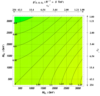
where and stands for (gluon) and (quark). These transcendental equations are solved numerically for the KK masses of the level ‘1’ KK gluon and quarks. The variations of the masses are plotted in figure 1 as a function of .

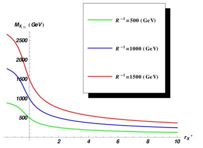
By virtue of equation (35), this dependence is blind to . It is interesting to note that for , signifying the actual KK mass to be larger than . The reverse is true for . As we can see from this panel that the variation flattens up quickly with increasing .
In the right panel of figure 1 we show the actual variations of KK masses (i.e., of ) for level ‘1’ KK gluon/quark for three given values of . This plot readily follows from the one in the left panel using the relation between and as indicated above. This also reveals that a particular mass-value for the KK gluon (quark) could arise from different combinations of and () which is further illustrated in figure 2 for a continuous range of .
This leads us to explore the isomass contours in the plane as illustrated in figure 2. This shows clearly how similar values of KK masses can be obtained for different combinations of and . Note that the straight line represented by (parallel to the -axis) cuts the mass contours at values of equal to the mass-value of the contour. This is in conformity with figure 1.
We give a quantitative summary for the KK masses of level ‘1’ KK gluon/quark in table 1 by providing some concrete numbers. represents the solutions of equation (35) for reference input values of which are independent of (as discussed earlier in this subsection). The actual KK masses are simple products of and . One such set of actual masses is shown for GeV in table 1.
In the above discussion we have taken a simplistic approach as far as the masses of the level ‘1’ KK quarks are concerned. It should be kept in mind that the mass-eigenvalues of the KK quarks would be evaluated from in equation (31). In general, the two eigenvalues are not degenerate because of the presence of non-vanishing overlap integrals like , etc. which are by themselves dimensionless and are also governed by dimensionless parameters like , , etc. When contrasted with mUED, this is a clear new feature appearing in the framework of UED with brane-localized terms. However, as can be seen from equation (31), the mass-splitting is proportional to the value of the corresponding zero-mode quark mass and thus negligible for the level ‘1’ KK quarks from the first two generations. In this limit, the mass eigenvalues () becomes identical to the KK mass (). On the contrary, corresponds to the physical mass of .

| (for ) | ||
|---|---|---|
| -1.5 | 1.771 | 1771 |
| -1.0 | 1.654 | 1654 |
| -0.5 | 1.386 | 1386 |
| 0.0 | 1.000 | 1000 |
| 0.5 | 0.767 | 767 |
| 1.0 | 0.638 | 638 |
| 2.0 | 0.500 | 500 |
| 5.0 | 0.339 | 339 |
| 10.0 | 0.246 | 246 |
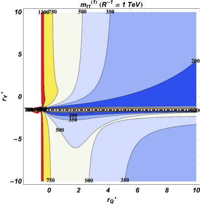
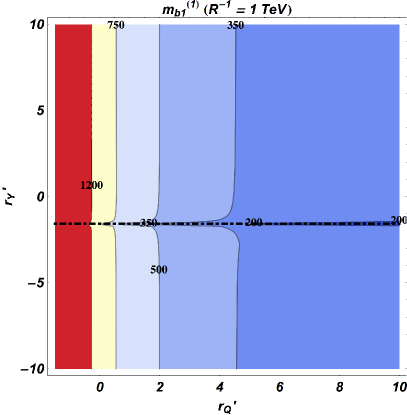
The phenomenon is not quite unexpected though since the effect under consideration originates in the Yukawa sector of the theory. Thus, such an effect will be appreciable for only the KK top quarks and to a far lesser extent for the KK bottom quarks. In the left plot of figure 3 we illustrate the effect for the lighter top quark with the help of isomass contours that show significant, nontrivial dependence of the mass on in addition to that on for a given value of (= 1000 GeV). The right panel of figure 3 is for the case of lighter level ‘1’ KK bottom quark. This one clearly reveals that for level ‘1’ KK quarks corresponding to the lighter SM quarks, the dependence of their masses on is small. Thus, these two plots collectively help one estimate the quantitative role of in the phenomenon.
As discussed in the beginning of section 2.2, at around the values of rise sharply and get divergent. In both plots of figure 3, this results in a thin strip of region about this value of over which there is no physical solution. Further, as mentioned at the end of section 2.2, because of the extremal situation it can lead to, close to its limiting value of can have non-trivial bearing even on the properties of the KK quarks of light flavours, at least, in principle.
Further, the possibility of level-mixing between similar KK-parity states driven by the brane-localized Yukawa term (as noted from equation (28)) emerges as an interesting feature of the top quark sector whose phenomenology could be rather rich in such a scenario. Our preliminary investigation into the subject reveals that mixing between level ‘0’ and level ‘2’ top quarks can be a priori significant. Such a mixing could potentially trigger an appreciable shift in the mass of the level ‘2’ top quark and make the same phenomenologically interesting at the LHC. Moreover, as could be expected, the SM top mass receives contribution from such a mixing. Thus, refined experimental estimates of the mass of the SM top quark from Tevatron Brandt:2012ui and the LHC Silva:2012di would inevitably constrain the parameters of the nmUED scenario we are considering here. A detailed study of the sector involving the KK quarks from the third generation including the role of level-mixing is beyond the scope of this paper and would be taken up separately in a future work.
3.2 Interactions involving level ‘1’ KK gluons and quarks
In this subsection we discuss the other important aspect of the framework, viz., the couplings involving the KK gluon and KK quarks. Here again, we limit ourselves only to the first KK level.
4D QCD coupling is defined as
| (36) |
Quartic interaction involving four level ‘1’ KK gluons is somewhat non-trivial and gets modified by the presence of brane-localized terms. However, it is rather inconsequential for LHC phenomenology and hence we do not discuss this any further. All other self-coupling terms involving level ‘1’ KK gluon and SM gluon (both 3-point and 4-point ones) remain the same as in mUED.
Next, we turn to the case of the interaction involving a level ‘1’ KK gluon and a level ‘1’ KK quark along with an (level ‘0’) SM quark. Here we comment on the forms of the bi-unitary matrices and that diagonalize the mass matrix for level-1 KK quarks where ‘’ refers to the quark-flavour. For (almost) mass-degenerate KK quarks (in the limit of which we adopt for studying the KK quarks corresponding to lighter SM flavours), and can be shown, to a very good approximation, to have the following form that reflects maximal mixing:
| (37) |
except for the case of .333This general form of the matrix is used in our subsequent analysis. It should be noted that this expression is qualitatively different from its mUED counterpart for which it is an unit matrix (see equation (40)) and this cannot be seen as a limiting case (i.e., ) of the former. In the case of conventional UED scenarios without brane-localized terms, one finds the mass-eigenvalues to be exactly degenerate (before radiative correction to the masses) and these matrices look like:
| (38) |
which include chiral rotation and the mixing angle is fixed by
| (39) |
where is the mass of the ‘’ th flavour SM quark. The difference in form of the matrices presented in equations (37) and (38) owes its origin to the difference between ‘approximate degeneracy’ and ‘exact degeneracy’ of the mass-eigenvalues of the quarks. Further, it may be noted that for the five light flavours, . Thus, use of equation (39) reduces equation (38) to the following trivial form:
| (40) |
whose form is different from that of equation (37).
Using equation (2), the 4D effective action depicting the quark-gluon interaction up to the first KK level can be written down as follows:
| (41) |
where the superscripts in parenthesis indicate the KK level. represent the quark mass-eigenstates at the first KK level, is the generic flavour-index and -s are the elements of the matrices in equations (32), (37). The latter can now be rewritten in the following general form:
| (42) |
The first term in equation (41) gives the usual interaction of the SM gluon with a pair of SM quarks. The next two terms give the interactions of the SM gluon with two different pairs of mass-eigenstates of level ‘1’ KK quarks and these are identical to their mUED counterparts. This is because they are governed by the overlap integral
| (43) |
which reduces to , the normalization factor in equation (36)) by virtue of the manifest identity in equation (18). The only deviation that occurs is in the case of an SM quark interacting with a level ‘1’ KK quark and a level ‘1’ KK gluon. The concrete form of the deviation (with respect to the mUED case) can be shown to be as in equation (44).
| (44) |
The factor is dimensionless and hence does not depend upon which is a dimensionful parameter. In fact, is implicitly governed by the dimensionless parameters and through the variables appearing in equation (44). This is a rather complicated dependence and its concrete profile has a rich structure as shown in figure 4. In the limit , it can be shown that which is the mUED.
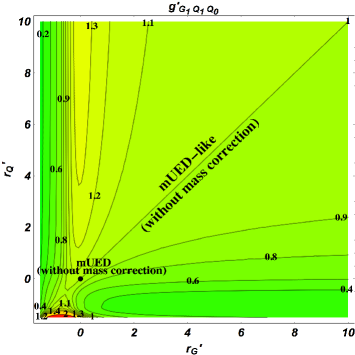
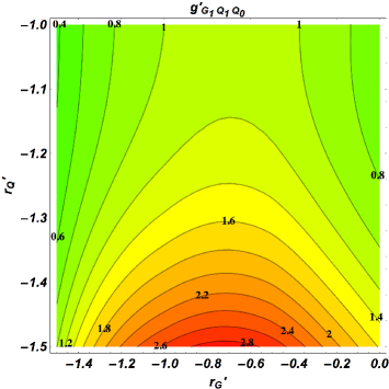
In figure 4 we present the contours of the deviation factor presented in equation (44) in the plane. The figure on left illustrates the contours over larger ranges of values for and . It is to be noted that along its diagonal () the deviation is exactly equal to 1 implying the coupling to be equal to that in the mUED.444The scenarios residing on the diagonal thus have degenerate KK masses which are different from those expected in a UED scenario without BLT (loosely indicated as mUED in the plot) for any given value of . We already assumed that in general, BLTs contribute dominantly to the KK masses when compared to the radiative corrections. The mUED scenario is defined only with the latter ones. Hence, on the diagonal, the scenarios are “mUED-like”. The coupling has a much richer structure at very low values of and close to the origin of the figure (indicated by blots in red and yellow) as both parameters approach their limiting value of . This is perhaps best understood if we just look at the form in equation (44) for which both and blow up at the said value. A closer look into this region is offered by a zoomed-up view in the right frame of figure 4.
To probe further into the generic aspects of correlated variations of the KK masses and the deviations in coupling from the mUED value, it would be useful to follow up with a study showing their mutual variation. This is pertinent since, as indicated above, the masses of the KK-quark and KK-gluon (we restrict ourselves to level ‘1’ KK excitations only) are also functions of and as does the deviation-factor. The only difference is that while the masses do vary with , the deviation-factor does not.
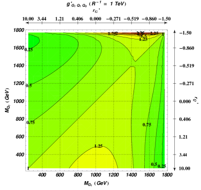
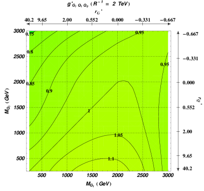
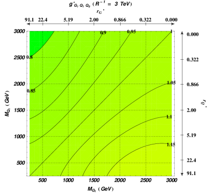
Thus, analogous to figure 4, contours of fixed deviations in the couplings can be drawn but this time in the plane with as a parameter. Such variations are shown in figure 5. In the top panel of figure 5, from left to right, we present the case of TeV and 2 TeV while in the bottom panel the corresponding ones illustrate the cases for TeV and 5 TeV, respectively. In order to facilitate the correspondences between the brane parameters and the masses of the respective excitations for different values of , the ranges of (along the abscissa) and (along the ordinate) are indicated on the top and the right of each of these plots. In both cases, the diagonal represents the contour for . Under the hood, the geometrical origin of the diagonal has a common thread to that in the left panel of figure 4, i.e., for , although the ranges considered for them are different from the earlier case. The small region in yellow and red close to the top-right corner of the top-left plot in figure 5 corresponds to the bottom-left corner of the left plot in figure 4.
For figure 5, the criteria for choosing the mass-ranges for the level ‘1’ gluon and quarks are, in turn, primarily based on the tentative reach of LHC ( TeV) running at the centre of mass energy of 14 TeV and then, choosing not too large values of and for different values of considered for these plots. Recall that, in the scenario we are considering in the present work, equal values of and , for a given result from equal values of and , respectively. Thus, as is clearly seen from figure 5, degenerate masses occur along the diagonal. As pointed out in the context of figure 4, here also, by the same token, mUED-like scenarios live close along the diagonals.
Figure 5 tells us that different combinations of masses for level ‘1’ gluon and level ‘1’ quarks would correspond to very specific values of the deviation-factor for the modified coupling. The deviation can go either way, i.e., . However, the correspondence between masses and the deviation in coupling is specific to the value of , as can be understood by comparing the plots presented in figure 5. We like to emphasize that this correspondence, in principle, could be exploited at the LHC to extract information on the parameters of the scenario. For example, if the masses in context can be known and the relevant cross sections can be estimated from the data, these could be used to determine the deviation in coupling.555Extracting a somewhat precise information about the deviation in coupling could be a challenging task at a hadron collider. This is because any attempt to understand this from a total yield (where all production processes contribute) would inevitably involve the decay-patterns of the originally produced new-physics excitations. Extracting some concrete information from within such a milieu requires further assumptions over the scenario and thus, the exercise may become heavily ‘model-dependent’. However, the situation is expected to be much under control in an extremely constrained scenario like the mUED where the production cross sections could very well be related to the decay-patterns of the produced particles. This is the case with us since we are trying to measure a deviation of the coupling from its mUED value. Since this deviation, when combined, with the information on the masses, has a unique relationship to in the current scenario, the latter can also be determined subsequently. The information thus obtained on , in turn, can be employed to determine the values of and since these determine the masses which are, by now, known.
To be convinced that such an approach would work, one has to demonstrate quantitatively that the value of can be estimated reasonably correctly. There are prima facie evidence that such an estimate would be unambiguous. This follows from the observation that neither the contours in figure 4 nor the same in figure 5 intersect each other. In table 2 we demonstrate the situation with some actual numbers for two different values of which one might be able to extract from experiments. The number presented in the table are picked up directly from the contour-plots in figure 5. Note that the values 0.85 and 1.1 that are chosen for in table 2 could result in deviations from the nominal values of the cross sections (which go as ) for the strong production modes at the LHC. This kind of a departure can be expected to be measured efficiently enough and thus can be used for further inferences. It is then informative to find from table 2 that for an experimentally estimated value of and for a known set of masses for the KK gluon and KK quarks, the value of is pretty distinct and thus can be estimated unambiguously.
| (TeV) | (GeV) | (GeV) | |
|---|---|---|---|
| 2 | 835.1 | 2724.3 | |
| 0.85 | 3 | 840.9 | 2407.6 |
| 5 | 1246.1 | 2819.1 | |
| 2 | 1820.0 | 500.0 | |
| 1.1 | 3 | 2019.5 | 1036.0 |
| 5 | 2121.7 | 989.6 |
4 Phenomenology at the LHC
In this section we discuss the cross sections of the level ‘1’ KK gluon () and quarks () of the nmUED scenario produced via strong interaction at the LHC. Hereafter, we use simplified notations, and , to denote the physical masses of the level ‘1’ KK gluon and quarks, respectively. The patterns are explained by relating them to the features of the scenario as discussed in detail in sections 3.1 and 3.2. We then proceed to contrast the production-rates with the corresponding ones from mUED and SUSY. We also discuss at length the overall implications of such an nmUED scenario whose signals can be faked by the latter two.
4.1 Production cross sections for level ‘1’ KK gluon and quarks
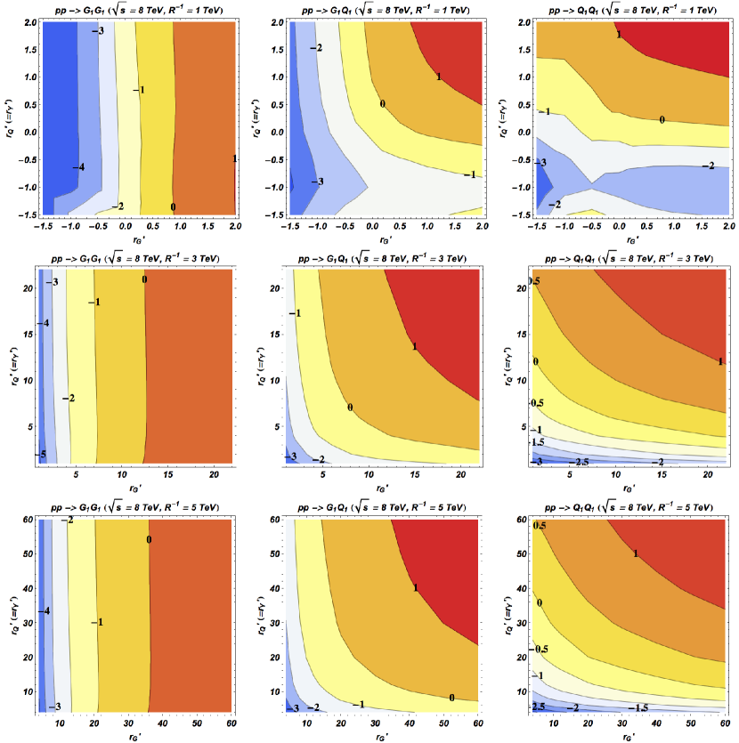
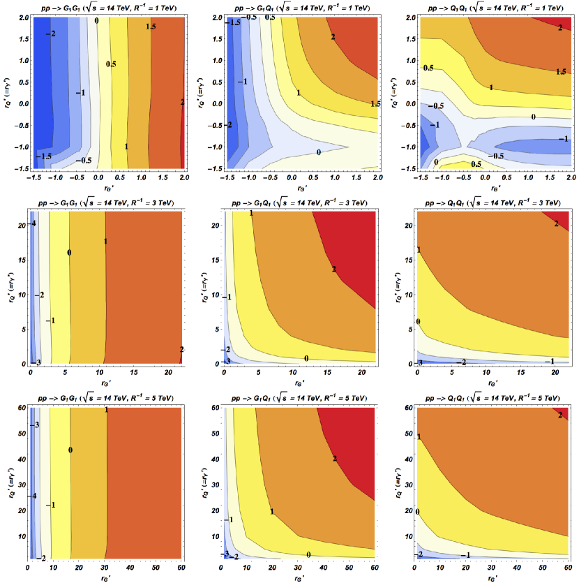
In figures 6 and 7 we present the cross sections for different final states for the 8 TeV and 14 TeV runs of the LHC, respectively, in the plane. Results for generic final states like , and are laid out in separate columns (from left to right) while separate rows are used to present the results for 1 TeV, 3 TeV and 5 TeV (from the top to the bottom). The final state indicated by includes contributions from both and while under we combine the rates from , and . The rates include contributions from five flavours of level ‘1’ KK quarks that correspond to five light SM quarks. For these states, as pointed out in sections 3.1 and 3.2, the role of is not significant except for some extremal cases, e.g., when , for smaller . Hence, we adopt a simplifying scheme where we set while analyzing these excitations at the LHC. Also, the contributions from both -doublet and -singlet varieties of KK quarks are included. On the other side of the story, we have seen in section 3.1 that the top quark sector turns out to be rather special thanks to crucial interplay of , and and to the possibility of significant level-mixing. This would render the phenomenology of the KK top quarks at the LHC rather rich. Given the intricacies involved, the analysis of this sector deserves a dedicated study. This will be taken up in a future work.
The cross sections are calculated using MadGraph-5 Alwall:2011uj in which the strongly interacting sector of the scenario is implemented through FeynRules Christensen:2008py via its UFO (Universal FeynRules Output) Degrande:2011ua ; deAquino:2011ub interface. The mUED implementation Datta:2010us of CalcHEP Pukhov:2004ca has been used for cross checks in appropriate limits and for some actual computation of cross sections in mUED. We used CTEQ6L Pumplin:2002vw parametrization for the parton distribution function. The factorization/renormalization scale is fixed at the sum of the masses of the final-state particles. In the remaining part of this work, we refer only to the physical masses . These are the degenerate mass-eigenvalues obtained by diagonalizing the KK quark mass-matrix in the presence of brane-localized Yukawa terms and practically same as the KK masses for the light quark flavours.
Some features common to both figures 6 and 7 are as follows:
-
•
the maximum value of the mass for the level ‘1’ KK gluon and quarks considered for TeV (14 TeV) run of the LHC is 2 TeV (3 TeV) which happens to be the tentative (perhaps, optimistic) reach of LHC running at this center of mass energy. The conservative lower limit of the masses that has gone into the analysis is 500 GeV,
-
•
for given values of , the various ranges of and in different rows ensure and in the above-mentioned ranges,
-
•
to capture cross-sections varying over orders of magnitude, the contours are drawn after taking the logarithm (to base 10) of the cross sections. We, thus, encounter negative-valued contours in these figures,
-
•
for final states containing one or more level ‘1’ KK quark (the second and the third columns), the contour values, (i.e., the cross sections) rise along the diagonal connecting the bottom-left and the top-right corners of the plots. This can be understood in terms of decreasing and as both and increase in that direction,
-
•
the variation in the production (the first column) has a curious trend when compared with the final-states having . The parallel, vertical stripes (except in some region with only for low ( TeV)) imply that the cross-sections almost do not vary with . This means they are insensitive to variations in . This is because the event rate for this final state is dominated by the -channel (gluon-fusion) subprocess where plays no role unlike in the -channel where the latter can appear as a propagator. Hence, we see a gradual, steady increase in rates only with increasing , i.e., with decreasing which is quite expected.
-
•
the local dependence of the rate on , for and TeV, shows a different trend. In this region (from the deep blue to the white passing through the light blue region), the rate grows in a direction of increasing which is somewhat not so intuitive. It is instructive to observe that for such a region, also turns out to be relatively heavy (since, ). Our probe into the phenomenon revealed that over this region the -channel contribution becomes important666Presumably, this happens since a larger requires a larger , in turn resulting in a lower partonic flux for the gluon in the protons that ultimately results in a suppressed contribution from the -channel. and the relative values of and are such that a perceptible destructive interference takes place between and channels. Note also that with getting extremally large over this region (see figure 4) of the parameter space, the overall situation gets further compounded,
-
•
the explanation holds for any final state that receives significant contributions from subprocesses initiated by gluon(s). Thus, it is not unexpected that rates for final state show a similar behaviour in the said region of the parameter space while the same for the level ‘1’ quark-pair final state, dominated by (which is not gluon-induced), though rich in feature, do not show such a trend very clearly,
-
•
for the -pair final state, one finds that in the region of low () the contours of larger cross sections reappear as one goes further down in . This seems to be a result of extremally large value of which can be understood from the region shaded in red in the right plot of figure 4. Closer inspection reveals that the small, yellow contour at the bottom of these plots exactly correspond to the region of parameter space shaded in red in figure 4. In this region, naively, the boost in cross section can be up to a factor which turns out to be ,
-
•
as we go from production to production passing through production the contours get flattened up in an anti-clockwise direction. This is easy to understand in terms of an increased dependence of the rates on and hence, on ,
- •
-
•
negative values of and are not considered for =3 TeV and 5 TeV cases since these take and far above the LHC reach. Thus, as we do not enter the “exotic” part of the parameter space (with both ), we do not see any special variation in the contour-patterns at lower values of and .
The only major difference of a generic nature that we see between the results presented in figures 6 ( TeV) and 7 ( TeV) is that for similar values of and , i.e., for similar values of and for a given , the rates are higher for the 14 TeV run, as expected.
4.2 mUED vs nmUED vs SUSY
In this subsection we take up the interesting possibility of mUED and nmUED faking each other and faking SUSY as well. This is reminiscent of the possibility of UED faking SUSY Cheng:2002ab where one talks about a situation in which the final state masses happen to be consistent with a mUED-like spectrum Datta:2005vx ; Smillie:2005ar . There, SUSY being a less constrained scenario, this is the natural set up to study its faking by mUED. Thus, with more free parameters in the scenario, nmUED may enjoy a more direct parallel to SUSY when being compared with mUED.777 Going one step further, it may be said that faking between UED and SUSY tend to get more complete Datta:2005zs ; Datta:2005vx with an nmUED-type scenario for which the masses of the KK excitations may take almost any arbitrary values. In this sense, it may be interesting to note the apparent contrast in the naming schemes for scenarios in SUSY and those involving a UED framework. In the case of SUSY, the minimal version is the least constrained one (with too many free parameters) while the same for UED is the one which is its most constrained incarnation with only two (three, with level ‘0’ Higgs mass parameter) parameters.
In table 3 we compare the cross sections for the production of level ‘1’ KK gluon and quarks as obtained from the mUED scenario and the nmUED version we are studying in this work at the LHC with TeV. Assuming that the ballpark values of the masses of these excitations could be anticipated once a positive signal is found at the LHC, we fix these masses to carry out the analysis.
The reference values for the masses employed in table 3 are GeV, GeV and GeV. These are obtained in the mUED scenario by setting GeV and . For the nmUED scenario, we require the level ‘1’ gluon mass to be the same as in the case of mUED while for the doublet and singlet KK quarks we take a common value which is almost equal to the singlet one in mUED. Note that, in the absence of radiative corrections, the masses of the doublet and singlet KK quarks are the same in the nmUED scenario under consideration and both are determined by the brane-localized parameter . Such an nmUED spectrum is generated for different by suitably tuning the brane-localized parameters and .
A priori, a comparison of cross sections from the two scenarios having similar spectrum assumes a special significance since the brane-localized parameters, and , not only control the KK masses but also affect their couplings. These are discussed in sections 3.1 and 3.2 with illustrations (see figures 4 and 5). It can be gleaned from table 3 that except for the case where with GeV and leaving out the -pair final state, the cross sections for the rest are within % of the corresponding mUED values. For these cases, the reason of such a closeness in cross sections can be understood in terms of the small deviation of the strong coupling from the mUED case which is quantified by and indicated in column 2. The smallness of the deviation in is ensured by the requirement of near-identical values of and in nmUED that reproduce the characteristic splitting between the masses of the KK gluon and the quarks in mUED.
On the other hand, the case for the -pair production is somewhat interesting. There, the cross sections are insensitive to variation in in contrast to what we see in case of other final states as we move on from =700 GeV. This may be attributed to the fact that the modified coupling given by only appears in the -channel while the process gets dominant contribution from the -channel. Moreover, unlike the previous cases, here, a marked difference is noticed between the cross sections for the mUED and the nmUED scenarios with the nmUED cross section ( pb) being smaller than the corresponding mUED value ( pb). The reason for this can be traced back to the particular chiral structure of the interaction vertex originating from the action in equation (41) that contains the elements -s of the matrices (see equations (37), (40) and (42)).
| mUED Parameters | GeV, | ||||||
|---|---|---|---|---|---|---|---|
| mUED/SUSY Mass (in GeV) | = 1220 = 1154 = 1133 | ||||||
| Cross sections (in pb) | |||||||
| Final states | |||||||
| mUED | 0.216 | 1.250 | 0.082 | 1.132 | 0.009 | 0.403 | |
| =700 GeV | |||||||
| =0.627 | 0.178 | 0.503 | 0.032 | 0.177 | 0.001 | 0.173 | |
| =1000 GeV | |||||||
| =1.035 | 0.172 | 1.349 | 0.085 | 1.277 | 0.009 | 0.432 | |
| =1500 GeV | |||||||
| nmUED | =0.37 | ||||||
| =0.54 | |||||||
| =1.033 | 0.173 | 1.364 | 0.086 | 1.303 | 0.010 | 0.438 | |
| =2000 GeV | |||||||
| =1.15 | |||||||
| =1.43 | |||||||
| =1.026 | 0.171 | 1.336 | 0.084 | 1.262 | 0.009 | 0.427 | |
| =2500 GeV | |||||||
| =2.13 | |||||||
| =2.56 | |||||||
| =1.019 | 0.172 | 1.326 | 0.083 | 1.233 | 0.009 | 0.421 | |
| SUSY (MSSM) | 0.019 | 0.181 | 0.012 | 0.153 | 0.001 | 0.054 | |
The differences in the cross sections, as we see from table 3, for the mUED and the nmUED scenarios, are not big enough for the LHC to signal a clear departure from one or the other of the two competing scenarios. Thus, it turns out that if a spectrum is compatible with the mUED scenario, it would not be easy to rule out a non-minimal version of the UED solely based on such a study. Of course, it may happen that other simultaneous studies involving the electroweak sector could help distinguish between the two.
The last line in table 3 shows the corresponding cross sections in a SUSY scenario (based on Minimal Supersymmetric Standard Model (MSSM)). The level ‘1’ KK excitations of the UED scenarios are substituted by their counterparts in SUSY: the KK gluon by the gluino, the -doublet quark by the left handed squark and the -singlet quark by the right handed squark. It is well known that, for identical mass spectra, UED production cross sections are generically larger than that for the analogous SUSY processes (by roughly a factor between 7 and 10). This is partly related to the structure of the UED matrix elements and the extra helicity states that UED excitations possess when compared to an analogous final state in SUSY. Even then, it is interesting to find that for (the first entry for the nmUED case in table 3), cross sections in some of the final states could approach the SUSY values. Thus, the total rate for strongly produced particles ceases to be a good enough indicator for the underlying scenario. This brings the alleged faking to an almost complete level. Note that this kind of a possibility does not arise in mUED. This again highlights how the correlation between masses and the couplings of the KK excitations in the nmUED scenario could shape the phenomenological situation in an interesting and involved way.
4.3 Decays of level 1 KK gluon, quarks and electroweak gauge bosons
In this section we discuss in brief the decay patterns of the level 1 KK gluon and quarks. When the KK gluon is heavier than the KK quarks (mutually degenerate for the lighter generation of the quarks), it decays to final state with 100% branching fraction. Thus, cascades are governed by the decay of the level 1 KK quarks which, in turn, decay to level 1 electroweak (EW) gauge bosons, and in two-body modes. On the other hand, for , level 1 KK quark undergoes 2-body decays to KK gluon and and . The KK gluon, in turn, decays to SM quarks and the above set of electroweak KK gauge bosons via 3-body modes.
We work with an electroweak sector at the first KK level (comprising of the gauge bosons, the charged leptons and the neutrinos) which is reminiscent of mUED with corrected masses Cheng:2002iz , that are essentially determined by . This can be seen as a limit of an electroweak sector in nmUED with vanishings BLTs. This is in line with the main goal of the present work as we focus on the role of BLKTs in the strongly interacting sector only. The resulting framework could thus be considered as a suitable benchmark (with only two BLKT parameters, and ) for initiating a phenomenological analysis of the nmUED at the LHC. The interaction vertex ( being the level ‘1’ electroweak gauge boson) that takes part in electroweak decays of the level ‘1’ KK quarks gets modified and follows from equation (44) with . Of course, more involved studies in scenarios having BLTs for the electroweak sector are highly warranted since such scenarios could emerge as perfect imposters of their popular SUSY counterparts.
With this assumption, and always decay to leptonic modes, i.e., and . is the lightest KK particle (LKP) and is stable. The only requirement to ensure these in nmUED is to set and in a way such that and do not become lighter than these electroweak bosons. This necessarily constrains the ranges of and that such a framework can take.
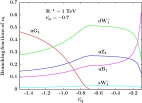
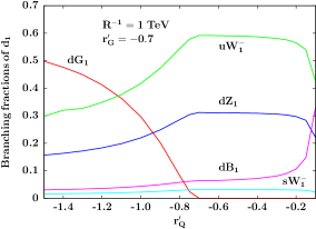
In figure 8 we present the branching fractions of the up and down type KK quarks as functions of and for fixed values of (1 TeV) and (-0.7). Each plot covers a range in for which both hierarchies between and are realized. Note that the decay widths (and the branching fractions) of the two mass eigenstates for each type of KK quark are very similar since they result from nearly maximal mixings of the weak eigenstates (see equation 37). It is clear that for , the KK quarks may dominantly decay into KK gluon with branching fractions reaching up to 50% before dropping quickly as quark mass increases. For a reverse hierarchy, the KK quarks only have 2-body electroweak decays. Among these, decays to Cabibbo-enhanced dominate followed by decays to , and Cabibbo-suppressed modes. The difference between electroweak branching fractions of the and the -type KK quarks stems solely from the difference in their hypercharges which only affects their decay widths to . It can be seen from figure 8 that the peak branching fraction to could be between 50% and 60% for the and the -type KK quarks, respectively. The average branching fraction to is found to be between 20% and 30% in the range of where electroweak decays dominate for the two species of quarks. Branching to tends to remain at around 20% (10%) or less for the -type (-type) quark before it shoots up as the quarks become lighter (from left to right) and the splitting between them and and become smaller. However, since the EW gauge boson masses are solely determined by , all three EW decay modes remain healthy over entire range of .
Note that the branching fractions of the KK quarks to the stable LKP () is on the lower side and they hardly dominate (except in extreme corners of the parameter space). This is in stark contrast to mUED (or, for that matter, SUSY scenarios) where the right chiral level 1 KK quarks (right chiral squarks) decay almost 100% of the time to LKP (bino-like LSP) when their strong decays to level 1 KK gluon (gluino) are closed. Later, we will see that this can have major implications for the relative rates in different final states when compared to contending scenarios.
As mentioned earlier, for , KK gluon decays to level 1 EW gauge bosons (, and ) in three-body modes via off-shell KK quarks. The variations of these branching fractions with respect to (or ) are expected to be flat. This is because () appears in the primary vertex of these decays and in the propagator (through the KK quark mass) and these two affect all three body decay modes in a similar way. The branching ratios are governed by the secondary vertex and thus follow the same pattern as in the decay of KK quarks, i.e., branching to dominates over the other two while the same to is the least favoured.888However, there may be a situation in nmUED when splitting between and drops critically resulting in an enhanced branching to .
4.4 Exclusion limits
It is instructive to have a look at the current LHC data and understand to what extent they may constrain an nmUED scenario of the present kind. In absence of a complete implementation of the scenario in an event generator, we limit ourselves to a parton level analysis which would, for example, give a ballpark estimate of the exclusion limit for under a reasonable set of assumptions.999Note that thorough simulation-studies for even the mUED scenario are not yet existing in the literature. In principle, constraints can be derived on any subspace of the 3-dimensional space spanning over .
Here, we take up a recent ATLAS analysis :2012rz of the final state with jets plus missing energy (with vetoed leptons) at TeV and integrated luminosity of 4.7 fb-1. We refer to the exclusion they report for equal mass gluino and squarks in the CMSSM scenario which is 1360 GeV. It must be pointed out that a straight-forward comparison with the experimental data ultimately requires a thorough simulation (including the detector effects) of the nmUED scenario under consideration which should wait for a full implementation of the same in an event generator like MadEvent and/or others. Nonetheless, using the information we gathered in the last subsection, we can reasonably attempt to translate the above ATLAS bound to ballpark constraints on the nmUED scenario.
Towards this we find the value of cross section times branching fraction (before cuts) for GeV using the similar set of CMSSM parameters as in the ATLAS study. In the absence of a complete simulation (where one would be able to employ kinematic cuts), we rely on this number and treat the same as the upper bound on the cross section times branching fraction. The task is then to find the bound on the masses and/or the parameters of the nmUED scenario that satisfies this constraint.
To carry out the analysis, we break the same up in three distinct regions in the nmUED parameter space having , and . Since we are not in a position to use kinematic cuts employed in the ATLAS analysis, the minimum requirement for being able to compare the nmUED results with the ATLAS study is to ensure the the kind of nmUED-spectra that result in hard enough jets and missing energy so that the ATLAS acceptances/efficiencies would hold safely.101010The spectra for this analysis are so chosen that for unequal masses for and , the mutual splitting between them as well as the splitting between the lighter one between and and the LKP is around 200 GeV. This would ensure (in absence of a full-fledged simulation with detector effects) jets from both primary and secondary cascades and the missing transverse energy to be hard enough to pass strong ATLAS cuts.. Thus, the constraints we obtain for the nmUED scenario could only be conservative and can be improved with help of a dedicated simulation. It is found that GeV could be ruled out for while, for , the exclusion could at best be up to 900 GeV.111111Note that these bounds on are insensitive to the values of and as long as the spectral splittings demanded are satisfied. Qualitatively, this can be termed as the most stringent constraint that could be put on the three-dimension nmUED parameter space considered here. One may like to take note of the anomalous region of a terminally large negative with large for which the couplings become very strong and could over-compensate for the suppression in the cross section due to large . In this region, perhaps, a larger value of could be ruled out. For , the lower bound can be as high as 1.1 TeV. However, in that case, sensitivity would be higher in the signal region with not too many hard jets since strong 2-body decays are phase-space suppressed.
In any case, we find that the bounds are degraded for nmUED when compared to CMSSM. This is not unexpected because of lower yield in channel for nmUED. On the other hand, similar constraints on CMSSM are expected to be weaker from the analysis of leptonic final states while the same for nmUED would yield a more stringent bound.
4.5 The case for 14 TeV LHC
In this subsection we discuss in brief the pattern of yields in various multi-jet, multi-lepton final states accompanied by large amount of missing transverse energy. The reference values chosen for this discussion are TeV and which are the same as in 4.3. In table 4 we present the expected uncut yields (in fb) for these final states as varies. For the second and the third columns, while for the fifth and the sixth columns, . For the fourth column and hence . To highlight the contrast, in the last three column we present the corresponding numbers for the mUED cases where the scenarios are solely determined by , for all practical purposes.
It is seen from table 4 that yields for all the final states decrease as decreases except for when the same increases suddenly. The latter can be understood in terms of an abrupt increase (up to three-fold) in the modified strong coupling close to the boundary of the theoretically allowed nmUED parameter space (see figure 4). The increase in the coupling strength, in fact, (over-)compensates for the lowering of the strong production cross sections as increases with decreasing . The drop in the yields over the range is attributed to the increase in when the increase in strong coupling strength is limited to around 20%. Note also the sharp variation of the yields for all the final states when going from to . This is mainly due to a sharper rise in (by GeV) when compared to the columns to follow (for which the rises are by 125-135 GeV). On a closer look, the most drastic drop occurs for the final state. This is explained by referring to figure 8 where one finds that the decay branching fraction for that contributes actively to the said final state suffers by a huge margin when goes from -0.1 to -0.5. Another feature that emerges from table 4 is that the yields in the leptonic modes are more pronounced than that in the leptonically quiet mode. This can be understood from the fact that the branching fractions of the KK quarks and the gluon to and are much larger than that to and that and decay entirely into leptons and missing particles.
| Scenario | nmUED | mUED () | ||||||
|---|---|---|---|---|---|---|---|---|
| TeV | /spectrum in TeV | |||||||
| -0.1 | -0.5 | -0.7 | -1.0 | -1.5 | =1.0 | 1.4 | 1.6 | |
| (TeV) | 1.07 | 1.39 | 1.52 | 1.65 | 1.77 | |||
| 1.15 | 1.60 | 1.83 | ||||||
| 1.09 | 1.53 | 1.75 | ||||||
| 466 | 27 | 15 | 10 | 83 | 1396 | 158 | 50 | |
| 332 | 68 | 39 | 26 | 215 | 804 | 88 | 31 | |
| 143 | 62 | 35 | 22 | 205 | 371 | 42 | 15 | |
For the mUED part of figure 4 the chosen values of take care of the range of masses for KK quark/KK gluon that were used in the nmUED case. Note that the nmUED yields are computed for a fixed while varies. For (1.52 TeV) that we employ in nmUED, a similar in the two cases (1 TeV) gives larger yields for the mUED case. The reason is simple and as follows. The mUED spectrum is dominantly determined by and =1 TeV gives a much lighter ( TeV) KK gluon in comparison to the nmUED case in hand. Table 4 reveals that the masses are comparable in the two scenarios when in nmUED and TeV in mUED. There also one finds that the rates are appreciably smaller for the nmUED case the most drastic difference being in the final state. The reason behind this has been discussed earlier. On the other hand, the closest possible faking in rates occur in some of the leptonic modes for and with TeV in nmUED and TeV in mUED. However, it is crucial to note that the rates in the all jets final state can be used as a robust discriminator between nmUED and mUED scenarios.
Thus, the pattern that exists among the yields in different final states could already disfavour mUED. When aided by a more thorough knowledge of their yields over the nmUED parameter space gathered through realistic simulations, such a study would constrain the nmUED parameter space as well. Further, crucial improvements, either in the form of exclusion or in pinning down the region of the parameter space is possible if some of the masses involved can be known, even if roughly. Under such a circumstance, the data can be simultaneously confronted by SUSY scenarios and the so-called SUSY-UED confusion could be addressed rather closely. Clearly, this is a rather involved study and hence will be taken up in a future study.
5 Conclusions and Outlook
In this work we discuss the role of non-vanishing BLTs (kinetic and Yukawa) in the strongly interacting sector of a scenario with one flat universal extra dimension and their impacts on the current and future runs at the LHC.
We solve for the resulting transcendental equations for masses numerically and discuss in detail the resulting spectra as functions of and the (scaled) brane-localized parameters, and . Unlike in mUED where the mass spectrum is essentially dictated only by , and play major roles (in conjunction with ) in determining the same in the nmUED scenario. This opens up the possibility that much larger (smaller) values of (which, still could result in lighter (heavier) KK spectra) can remain relevant at the LHC when compared to mUED. Nontrivial deviations from the mUED are noted in the strong and electroweak interaction vertices involving the level ‘1’ quarks. The deviations are found to be functions of and only. Arguably, the most nontrivial implication of the presence of non-vanishing brane-localized terms is that both masses and couplings of the KK excitations are simultaneously controlled by these free parameters and thus, these become correlated. We demonstrate the same and discuss its possible implications at the LHC and contemplated on the role it may play in extracting the fundamental parameters of such a scenario.
We then study the basic cross sections for production of level ‘1’ KK gluon and KK quarks (excluding the KK top quark) as functions of the free parameters of the scenario at two different LHC-energies, 8 TeV and 14 TeV. It is noted that, when compared to the same in mUED, for a given , wildly varying yields are possible. This is because the final state KK gluon and quarks can now have masses freely varying over wide ranges. The top quark sector is kept out of the ambit of this work since the structure and the resulting phenomenology of the same are rather involved, as usual. On top of that, there is a new possibility of level-mixing triggered by BLTs. Thus, this sector deserves a dedicated study.
It is pointed out that even if the level 1 KK gluon and the quarks happen to have masses compatible with mUED, they could actually result from an nmUED-type scenario with a value of different from that in the mUED case. Although the presence of a coupling () with modified strength can signal an nmUED-like scenario, such departures are expected to be miniscule. This is since for a given , an mUED-like spectrum is obtained only with for which deviations in the said coupling remain negligible.
Further, an nmUED-type scenario where the masses of the KK excitations are much less constrained, can fake SUSY more completely than a conventional mUED scenario. Theoretically, one well-known approach to discriminate between these scenarios, is to compare the cross sections; the expectation being the same to be larger for UED for a given set of masses in the final state (noting that both scenarios have the respective couplings of equal strengths). However, it is unlikely that a SUSY-like spectrum (unless it is degenerate) could emerge from an nmUED scenario of the present type without making the deviation in coupling large from the corresponding SUSY values (which are identical to the corresponding SM or the mUED values). Thus, if , this may bring down an otherwise large nmUED cross section close to the SUSY value.
To get an idea of the actual rates for different final states (comprised of jets, leptons and missing energy) we computed the branching fraction of different excitations that appear in the cascades. For this we bring in an EW sector (with gauge bosons and leptons and neutrinos) which resembles mUED. Some contrasting features with respect to mUED and SUSY are noted in the form of inverted branching probabilities to jets and leptons. This would result in an enhanced (depleted) lepton-rich (jet-rich) events at the LHC in an nmUED-type scenario. The feature can be exploited for partial amelioration of the infamous SUSY-UED confusion. It was also demonstrated that the latest LHC data can rule out (conservatively) up to around 1 TeV under some reasonable set of assumptions. A rigorous framework for detailed LHC-analyses of such a scenario including the detector effects and complete implementation of the EW sector (with EW BLTs) in event generators like MadGraph is highly warranted. This would be the subject of a future work.
It should be kept in mind that the nmUED scenario considered in this work is of a rather prototype variety with some generic features governed by three to four basic parameters. This is a modest number for a new physics scenario. Hence, such a scenario is much more tractable than many of its SUSY counterparts. Nonetheless, this already offers a host of rich, new effects that can be studied at the LHC. Note that the brane-localized parameters we consider are all blind to flavours, the gauge quantum numbers and independent of the locations of the orbifold fixed-points they appear at. Moreover, wherever appropriate, we assumed some of them ( or , for that matter) are equal. Deviations from any of these assumptions would have important consequences. On the other hand, in the nmUED scenario, radiative corrections to the KK-spectrum can be expected to be somewhat significant just as they are in the case of conventional mUED. However, unlike in mUED where these corrections are the sole source of mass-splittings among an otherwise degenerate set of KK excitations, the nmUED spectrum may already come with a considerable splitting at a given KK-level even at the tree level, thus diluting the role of radiative corrections.
In any case, knowledge of the strong-production rates, supplemented with some crucial information on decays of involved KK excitations, lays the groundwork for initiating phenomenological studies of the nmUED scenario discussed in this work. The present work, thus, serves as a launch-pad to undertake a thorough analysis of such scenarios at the LHC.
Acknowledgments KN and SN are partially supported by funding available from the Department of Atomic Energy, Government of India for the Regional Centre for Accelerator-based Particle Physics (RECAPP), Harish-Chandra Research Institute. The authors like to thank P. Aquino, J. Chakrabortty, N. D. Christensen, O. Mattelaer and A. Pukhov for very helpful discussions on issues with FeynRules and CalcHEP and U. K. Dey for many helpful discussions. AD thanks Department of Physics, University of Florida, Gainesville, USA for his sabbatical-stint during which this project was initiated. The authors acknowledge the use of computational facility available at RECAPP and thank Joyanto Mitra for technical help.
Appendix
Appendix A Feynman rules
We write down the concrete forms of Feynman rules where we take all 4D momenta as incoming. Details of our conventions are given in section 3. Note that we omit the rule for the quartic coupling involving only since it is not important in LHC phenomenology.
| (45) | ||||
| (46) | ||||
| (47) | ||||
| (48) |
| (49) | ||||
| (50) | ||||
| (51) |
References
- (1) I. Antoniadis, “A Possible new dimension at a few TeV,” Phys. Lett. B 246 (1990) 377.
- (2) T. Appelquist, H. -C. Cheng and B. A. Dobrescu, “Bounds on universal extra dimensions,” Phys. Rev. D 64 (2001) 035002 [hep-ph/0012100].
- (3) G. Servant and T. M. P. Tait, “Is the lightest Kaluza-Klein particle a viable dark matter candidate?,” Nucl. Phys. B 650 (2003) 391 [hep-ph/0206071].
- (4) H. -C. Cheng, J. L. Feng and K. T. Matchev, “Kaluza-Klein dark matter,” Phys. Rev. Lett. 89 (2002) 211301 [hep-ph/0207125].
- (5) M. Kakizaki, S. Matsumoto, Y. Sato and M. Senami, “Significant effects of second KK particles on LKP dark matter physics,” Phys. Rev. D 71 (2005) 123522 [hep-ph/0502059].
- (6) M. Kakizaki, S. Matsumoto, Y. Sato and M. Senami, “Relic abundance of LKP dark matter in UED model including effects of second KK resonances,” Nucl. Phys. B 735 (2006) 84 [hep-ph/0508283].
- (7) F. Burnell and G. D. Kribs, “The Abundance of Kaluza-Klein dark matter with coannihilation,” Phys. Rev. D 73 (2006) 015001 [hep-ph/0509118].
- (8) K. Kong and K. T. Matchev, “Precise calculation of the relic density of Kaluza-Klein dark matter in universal extra dimensions,” JHEP 0601 (2006) 038 [hep-ph/0509119].
- (9) S. Matsumoto and M. Senami, “Efficient coannihilation process through strong Higgs self-coupling in LKP dark matter annihilation,” Phys. Lett. B 633 (2006) 671 [hep-ph/0512003].
- (10) M. Kakizaki, S. Matsumoto and M. Senami, “Relic abundance of dark matter in the minimal universal extra dimension model,” Phys. Rev. D 74 (2006) 023504 [hep-ph/0605280].
- (11) S. Matsumoto, J. Sato, M. Senami and M. Yamanaka, “Relic abundance of dark matter in universal extra dimension models with right-handed neutrinos,” Phys. Rev. D 76 (2007) 043528 [arXiv:0705.0934 [hep-ph]].
- (12) G. Belanger, M. Kakizaki and A. Pukhov, “Dark matter in UED: The Role of the second KK level,” JCAP 1102 (2011) 009 [arXiv:1012.2577 [hep-ph]].
- (13) H. C. Cheng, K. T. Matchev and M. Schmaltz, “Radiative corrections to Kaluza-Klein masses,” Phys. Rev. D 66 (2002) 036005 [hep-ph/0204342].
- (14) H. C. Cheng, K. T. Matchev and M. Schmaltz, “Bosonic supersymmetry? Getting fooled at the CERN LHC,” Phys. Rev. D 66 (2002) 056006 [hep-ph/0205314].
- (15) T. G. Rizzo, “Probes of universal extra dimensions at colliders,” Phys. Rev. D 64 (2001) 095010 [hep-ph/0106336].
- (16) C. Macesanu, C. D. McMullen and S. Nandi, “Collider implications of universal extra dimensions,” Phys. Rev. D 66 (2002) 015009 [hep-ph/0201300].
- (17) C. D. Carone, J. M. Conroy, M. Sher and I. Turan, “Universal extra dimensions and Kaluza-Klein bound states,” Phys. Rev. D 69 (2004) 074018 [hep-ph/0312055].
- (18) G. Bhattacharyya, P. Dey, A. Kundu and A. Raychaudhuri, “Probing universal extra dimension at the international linear collider,” Phys. Lett. B 628 (2005) 141 [hep-ph/0502031].
- (19) J. A. R. Cembranos, J. L. Feng and L. E. Strigari, “Exotic Collider Signals from the Complete Phase Diagram of Minimal Universal Extra Dimensions,” Phys. Rev. D 75 (2007) 036004 [hep-ph/0612157].
- (20) B. Bhattacherjee and A. Kundu, “Production of Higgs boson excitations of universal extra dimension at the large hadron collider,” Phys. Lett. B 653 (2007) 300 [arXiv:0704.3340 [hep-ph]].
- (21) B. Bhattacherjee, A. Kundu, S. K. Rai and S. Raychaudhuri, “Universal Extra Dimensions, Radiative Returns and the Inverse Problem at a Linear e+e- Collider,” Phys. Rev. D 78 (2008) 115005 [arXiv:0805.3619 [hep-ph]].
- (22) P. Konar, K. Kong, K. T. Matchev and M. Perelstein, “Shedding Light on the Dark Sector with Direct WIMP Production,” New J. Phys. 11 (2009) 105004 [arXiv:0902.2000 [hep-ph]].
- (23) S. Matsumoto, J. Sato, M. Senami and M. Yamanaka, “Productions of second Kaluza-Klein gauge bosons in the minimal universal extra dimension model at LHC,” Phys. Rev. D 80 (2009) 056006 [arXiv:0903.3255 [hep-ph]].
- (24) G. Bhattacharyya, A. Datta, S. K. Majee and A. Raychaudhuri, “Exploring the Universal Extra Dimension at the LHC,” Nucl. Phys. B 821 (2009) 48 [arXiv:0904.0937 [hep-ph]].
- (25) P. Bandyopadhyay, B. Bhattacherjee and A. Datta, “Search for Higgs bosons of the Universal Extra Dimensions at the Large Hadron Collider,” JHEP 1003 (2010) 048 [arXiv:0909.3108 [hep-ph]].
- (26) B. Bhattacherjee and K. Ghosh, “Search for the minimal universal extra dimension model at the LHC with =7 TeV,” Phys. Rev. D 83 (2011) 034003 [arXiv:1006.3043 [hep-ph]].
- (27) H. Murayama, M. M. Nojiri and K. Tobioka, “Improved discovery of a nearly degenerate model: MUED using MT2 at the LHC,” Phys. Rev. D 84 (2011) 094015 [arXiv:1107.3369 [hep-ph]].
- (28) K. Ghosh, S. Mukhopadhyay and B. Mukhopadhyaya, “Discrimination of low missing energy look-alikes at the LHC,” JHEP 1010 (2010) 096 [arXiv:1007.4012 [hep-ph]].
- (29) K. Nishiwaki, K. -y. Oda, N. Okuda and R. Watanabe, “Heavy Higgs at Tevatron and LHC in Universal Extra Dimension Models,” Phys. Rev. D 85 (2012) 035026 [arXiv:1108.1765 [hep-ph]].
- (30) A. Datta, A. Datta and S. Poddar, “Enriching the exploration of the mUED model with event shape variables at the CERN LHC,” Phys. Lett. B 712 (2012) 219 [arXiv:1111.2912 [hep-ph]].
- (31) K. Ghosh and K. Huitu, “Constraints on Universal Extra Dimension models with gravity mediated decays from ATLAS diphoton search,” JHEP 1206 (2012) 042 [arXiv:1203.1551 [hep-ph]].
- (32) G. Aad et al. [ATLAS Collaboration], “Search for Diphoton Events with Large Missing Transverse Energy in 7 TeV Proton-Proton Collisions with the ATLAS Detector,” Phys. Rev. Lett. 106 (2011) 121803 [arXiv:1012.4272 [hep-ex]].
- (33) K. Nishiwaki, “Higgs production and decay processes via loop diagrams in various 6D Universal Extra Dimension Models at LHC,” JHEP 1205 (2012) 111 [arXiv:1101.0649 [hep-ph]].
- (34) K. Nishiwaki, K. -y. Oda, N. Okuda and R. Watanabe, “A bound on Universal Extra Dimension Models from up to 2fb-1 of LHC Data at 7TeV,” Phys. Lett. B 707 (2012) 506 [arXiv:1108.1764 [hep-ph]].
- (35) G. Belanger, A. Belyaev, M. Brown, M. Kakizaki and A. Pukhov, “Higgs Phenomenology of Minimal Universal Extra Dimensions,” EPJ Web Conf. 28 (2012) 12070 [arXiv:1201.5582 [hep-ph]].
- (36) T. Kakuda, K. Nishiwaki, K. -y. Oda, N. Okuda and R. Watanabe, “Higgs at ILC in Universal Extra Dimensions in Light of Recent LHC Data,” arXiv:1202.6231 [hep-ph].
- (37) M. Battaglia, A. Datta, A. De Roeck, K. Kong and K. T. Matchev, “Contrasting supersymmetry and universal extra dimensions at the clic multi-TeV e+ e- collider,” JHEP 0507 (2005) 033 [hep-ph/0502041].
- (38) A. Datta, K. Kong and K. T. Matchev, “Discrimination of supersymmetry and universal extra dimensions at hadron colliders,” Phys. Rev. D 72 (2005) 096006 [Erratum-ibid. D 72 (2005) 119901] [hep-ph/0509246].
- (39) A. Datta, G. L. Kane and M. Toharia, “Is it SUSY?,” hep-ph/0510204.
- (40) J. M. Smillie and B. R. Webber, “Distinguishing spins in supersymmetric and universal extra dimension models at the large hadron collider,” JHEP 0510 (2005) 069 [hep-ph/0507170].
- (41) S. C. Park and J. Shu, “Split Universal Extra Dimensions and Dark Matter,” Phys. Rev. D 79 (2009) 091702 [arXiv:0901.0720 [hep-ph]].
- (42) C. -R. Chen, M. M. Nojiri, S. C. Park, J. Shu and M. Takeuchi, “Dark matter and collider phenomenology of split-UED,” JHEP 0909 (2009) 078 [arXiv:0903.1971 [hep-ph]].
- (43) K. Kong, S. C. Park and T. G. Rizzo, “Collider Phenomenology with Split-UED,” JHEP 1004 (2010) 081 [arXiv:1002.0602 [hep-ph]].
- (44) T. Flacke and C. Pasold, “Constraints on split-UED from Electroweak Precision Tests,” Phys. Rev. D 85 (2012) 126007 [arXiv:1111.7250 [hep-ph]].
- (45) G. -Y. Huang, K. Kong and S. C. Park, “Bounds on the Fermion-Bulk Masses in Models with Universal Extra Dimensions,” JHEP 1206 (2012) 099 [arXiv:1204.0522 [hep-ph]].
- (46) G. R. Dvali, G. Gabadadze, M. Kolanovic and F. Nitti, “The Power of brane induced gravity”, Phys. Rev. D 64 (2001) 084004 [hep-ph/0102216].
- (47) M. S. Carena, T. M. P. Tait and C. E. M. Wagner, “Branes and orbifolds are opaque,” Acta Phys. Polon. B 33 (2002) 2355 [hep-ph/0207056].
- (48) F. del Aguila, M. Perez-Victoria and J. Santiago, “Bulk fields with general brane kinetic terms,” JHEP 0302 (2003) 051 [hep-th/0302023].
- (49) F. del Aguila, M. Perez-Victoria and J. Santiago, hep-ph/0305119.
- (50) F. del Aguila, M. Perez-Victoria and J. Santiago, “Bulk fields with brane terms,” Eur. Phys. J. C 33 (2004) S773 [hep-ph/0310352].
- (51) F. del Aguila, M. Perez-Victoria and J. Santiago, “Physics of brane kinetic terms,” Acta Phys. Polon. B 34 (2003) 5511 [hep-ph/0310353].
- (52) A. Muck, L. Nilse, A. Pilaftsis and R. Ruckl, “Quantization and high energy unitarity of 5-D orbifold theories with brane kinetic terms,” Phys. Rev. D 71 (2005) 066004 [hep-ph/0411258].
- (53) F. del Aguila, M. Perez-Victoria and J. Santiago, “Effective description of brane terms in extra dimensions,” JHEP 0610 (2006) 056 [hep-ph/0601222].
- (54) T. Flacke, A. Menon and D. J. Phalen, “Non-minimal universal extra dimensions,” Phys. Rev. D 79 (2009) 056009 [arXiv:0811.1598 [hep-ph]].
- (55) T. Flacke, A. Menon and Z. Sullivan, “Constraints on UED from W’ searches,” Phys. Rev. D 86 (2012) 093006 [arXiv:1207.4472 [hep-ph]].
- (56) A. Datta, U. K. Dey, A. Shaw and A. Raychaudhuri, “Universal Extra-Dimensional models with boundary localized kinetic terms: Probing at the LHC,” arXiv:1205.4334 [hep-ph].
- (57) M. Schmaltz and D. Tucker-Smith, “Little Higgs review,” Ann. Rev. Nucl. Part. Sci. 55 (2005) 229 [hep-ph/0502182].
- (58) M. Perelstein, “Little Higgs models and their phenomenology,” Prog. Part. Nucl. Phys. 58 (2007) 247 [hep-ph/0512128].
- (59) F. Coradeschi, S. De Curtis, D. Dominici and J. R. Pelaez, “Modified spontaneous symmetry breaking pattern by brane-bulk interaction terms,” JHEP 0804 (2008) 048 [arXiv:0712.0537 [hep-th]].
- (60) C. P. Burgess, C. de Rham and L. van Nierop, “The Hierarchy Problem and the Self-Localized Higgs,” JHEP 0808 (2008) 061 [arXiv:0802.4221 [hep-ph]].
- (61) N. Haba, K. -y. Oda and R. Takahashi, “Top Yukawa Deviation in Extra Dimension,” Nucl. Phys. B 821 (2009) 74 [Erratum-ibid. 824 (2010) 331] [arXiv:0904.3813 [hep-ph]].
- (62) Y. Fujimoto, T. Nagasawa, S. Ohya and M. Sakamoto, “Phase Structure of Gauge Theories on an Interval,” Prog. Theor. Phys. 126 (2011) 841 [arXiv:1108.1976 [hep-th]].
- (63) C. Csaki, C. Grojean, H. Murayama, L. Pilo and J. Terning, “Gauge theories on an interval: Unitarity without a Higgs,” Phys. Rev. D 69 (2004) 055006 [hep-ph/0305237].
- (64) C. Csaki, C. Grojean, J. Hubisz, Y. Shirman and J. Terning, “Fermions on an interval: Quark and lepton masses without a Higgs,” Phys. Rev. D 70 (2004) 015012 [hep-ph/0310355].
- (65) O. Brandt [CDF and D0 Collaborations], “Measurements of the top quark mass at the Tevatron,” arXiv:1204.0919 [hep-ex].
- (66) P. Silva et al. [ATLAS and CMS Collaborations], “Recent results on Top quark Physics with the ATLAS and CMS experiments,” arXiv:1206.2967 [hep-ex].
- (67) J. Alwall, M. Herquet, F. Maltoni, O. Mattelaer and T. Stelzer, “MadGraph 5 : Going Beyond,” JHEP 1106 (2011) 128 [arXiv:1106.0522 [hep-ph]].
- (68) N. D. Christensen and C. Duhr, “FeynRules - Feynman rules made easy,” Comput. Phys. Commun. 180 (2009) 1614 [arXiv:0806.4194 [hep-ph]].
- (69) C. Degrande, C. Duhr, B. Fuks, D. Grellscheid, O. Mattelaer and T. Reiter, “UFO - The Universal FeynRules Output,” Comput. Phys. Commun. 183 (2012) 1201 [arXiv:1108.2040 [hep-ph]].
- (70) P. de Aquino, W. Link, F. Maltoni, O. Mattelaer and T. Stelzer, “ALOHA: Automatic Libraries Of Helicity Amplitudes for Feynman Diagram Computations,” Comput. Phys. Commun. 183 (2012) 2254 [arXiv:1108.2041 [hep-ph]].
- (71) A. Datta, K. Kong and K. T. Matchev, “Minimal Universal Extra Dimensions in CalcHEP/CompHEP,” New J. Phys. 12 (2010) 075017 [arXiv:1002.4624 [hep-ph]].
- (72) A. Pukhov, “CalcHEP 2.3: MSSM, structure functions, event generation, batchs, and generation of matrix elements for other packages,” hep-ph/0412191.
- (73) J. Pumplin, D. R. Stump, J. Huston, H. L. Lai, P. M. Nadolsky and W. K. Tung, “New generation of parton distributions with uncertainties from global QCD analysis,” JHEP 0207 (2002) 012 [hep-ph/0201195].
- (74) G. Aad et al. [ATLAS Collaboration], “Search for squarks and gluinos with the ATLAS detector in final states with jets and missing transverse momentum using 4.7 of TeV proton-proton collision data,” arXiv:1208.0949 [hep-ex].